Weak Solution of Renormalization Group Equation (Applications of Renormalization Group Methods in Mathematical Sciences)

Weak

Solution

of

Renormalization Group

Equation

Ken-Ichi Aoki,

Shin-Ichiro

Kumamoto and Daisuke

Sato*

$In\mathcal{S}$

titute

for

Theoretical

$Phy_{\mathcal{S}}ics$

,

Kanazawa University

Abstract

In the approach ofnon-perturbative renormalization group (NPRG), the

spon-taneous chiral symmetry breaking induces a singularity in its solution, e.g., the

flow of the 4-fermi coupling constant blows up at a critical renormalization group

(RG) scale. Thus, as long as directly solving the NPRG equation as a partial

differential equation, the RG flow cannot go beyond the critical scale to obtain

in-frared quantities such as the chiral condensates. In order to treat this singularity in a mathematically rigorous way, we introduce the notion of weak solution of the

NPRGequation. The weak solution is found togive auniqueglobal solution toward theinfrared limit, and wecancalculate infraredquantitieswithout any ambiguities.

1

Introduction

The almost 100 percent ofmassis originated from spontaneouschiral symmetry breaking

$(S\chi SB)$, while

a

few percent of

mass

is _{given by the so-called Higgs mechanism. The}

$S\chi SB$ is included by the strong interaction between quarks at the low energy scale which

is described by quantum chromodynamics (QCD). Because of the strong interaction, the

perturbationtheory does not work, and

so

we need non-perturbative methods such

as

the

lattice simulation and the Schwinger-Dyson (SD) approach.

In thisarticle, we usetheapproachof non-perturbative renormalization group (NPRG)

that is originatedfrom the Wilsonian idea. This approach does not have the sign problem

at finite chemical potential just like the lattice simulation, and can improve the gauge

dependence ofphysical quantities, which the SD approach suffers, in systematic

approxi-mations [1, 2].

For simplicity, we are limited to the analysis using the Nambu-Jona Lasinio (NJL)

model with a simplified discrete chiral symmetry, which is a low energy model of QCD

explaining the $S\chi SB$. Its Lagrangian is given by

$\mathcal{L}=\overline{\psi}\emptyset\psi-\frac{G_{0}}{2}(\overline{\psi}\psi)^{2}$,

(1)

where $\psi$ and $\overline{\psi}$ is

a quark field and an antiquark field, respectively Here the discrete

chiral symmetry is that the Lagrangian is invariant under the following discrete chiral

transformation:

$\psiarrow\gamma_{5}\psi, \overline{\psi}arrow-\overline{\psi}\gamma_{5}$. (2)

The chiral symmetry thus forbids the

mass

term $m\overline{\psi}\psi$ and the chiral condensates $\langle\overline{\psi}\psi\rangle.$

However, when the 4-fermi coupling constant $G_{0}$ islarger than

a

critical couplingconstant,

its strong coupling induces the $S\chi SB$. If using the

mean

field approximation, the critical

coupling constant $G_{c}$ is $4\pi^{2}/\Lambda_{0}^{2}$, where $\Lambda_{0}$ is the ultraviolet cutoff scale. Note that the

mean field approximation is equivalent to the self-consistency equation limited to the

large-N leading, where $N$ is the number of quarkflavors.

Many NPRG analyses of $S\chi SB$ have been performed by introducing the

bosoniza-tion ofthe multi-fermi interactions [3-6], which is the so-called auxiliaryfield method or Hubbard-Stratonovich transformation. However the analysis without the bosonization is difficult because in theRG procedure the 4-fermi coupling constant blows up at a critical

scale as a signal of $S\chi SB[7$,8$]$. Consequently we cannot go beyond the critical scale to

obtain infrared physical quantities such

as

the chiral condensates.

The goal of this article is to analyze$S\chi SB$ in theNPRG approachwithout introducing

the bosonization. Forthis goal

we

adopt themethod of weak solution [9], which has firstly

been introduced in the NPRG approach by the authors [10]. As the NPRG equation is

given byapartial differentialequation (PDE),the weak solution satisfiesthe integral-form

(weak) equation ofthe PDE. Since the weak solution is globally defined, it can include

singularities such

as

the explosive behavior of the 4-fermi coupling constant.

This article is organized

as

follows. InSect.2, webriefly explain the Wegner-Houghton

equation that is a formulation of the NPRG and the difficulty of the NPRG analysis of

$S\chi SB$ without the bosonization. In Sect3, the method of weak solution is adopted to

overcome

this difficulty. In Sect4, the bare

mass

of quark is introduced to define the

chiral order parameters. In Sect5, the method of weak solution is applied to the first

order phase transition at finite chemical potential, and the convexity of the effective

potential given by the weak solution is discussed. Finally we summarize this article in

Sect6.

2

Non-perturbative

renormalization

group

In theNPRG approach, a central object isthe Wilsonian effective action $S_{eff}[\phi_{)}\Lambda]$ defined

by integrating the microscopic degrees of freedom $\phi_{H}$ with momentums higher than the

scale $\Lambda$

:

$\int \mathcal{D}\phi_{H}e^{-S_{0}[\phi_{L_{\rangle}}\phi_{H},\Lambda_{0}]}=e^{-S_{eff}[\phi_{L},\Lambda]}$, (3)

where $S_{0}[\phi;\Lambda_{0}]$ is a bare action with the ultraviolet cutoff scale $\Lambda_{0}$. Now we parametrize

the cutoff scale $\Lambda$ by a dimensionless scale $t$ such that

$\Lambda(t)=\Lambda_{0}e^{-t}$. (4)

The $t$-dependence of the effective action $S_{eff}[\phi;\Lambda]$ is given by a NPRG equation

as

the

following functional partial differential equation:

$\partial_{t}S_{eff}[\phi;t]=\beta_{WH}[\frac{\delta S_{eff}}{\delta\phi}, \frac{\delta^{2}S_{eff}}{\delta\phi^{2}};t]$ , (5)

whichis calledthe Wegner-Houghton (WH) equation [11] (seeRef. [12] forthedetailform

suchas thechiral condensatesand theeffectivequarkmass, bysettingthe bare action$S_{0}$to

the initial condition at $t=0$ and solving it as a differential equation toward the infrared

scale $(tarrow\infty)$. Of course, it cannot be solved exactly, but various _{non-perturbative}

approximation to solve it are available.

In this article, theWHequation is applied to the NJL model (3). As anapproximation,

we restrict the full interaction space of the effective action $S_{eff}[\psi, \overline{\psi};t]$ to be the subspace

relevant to $S\chi SB$

as

follows:

$S_{eff}[ \psi, \overline{\psi};t]=\int d^{4}x\{\overline{\psi}\beta\psi-V_{W}(x;t)\}$ , (6)

whereascalarfermion-bilinearfield,$x=\overline{\psi}\psi$, is introduced. The potential term

$V_{W}(x;t)$ is

called the

fermion

potentialhere, whose initial conditionis setto $V_{W}(x;t=0)=(G_{0}/2)x^{2}$

according to the NJL Lagrangian(1).

In addition to the restriction ofthe interaction space, the large-N non-leading parts

of the WH equation(3) are ignored. Then, the NPRG equation for the fermion potential

in the large-N approximation is given by the following partial differential equation:

$\partial_{t}V_{W}(x;t)=\frac{\Lambda^{4}}{4\pi^{2}}\log(1+\frac{1}{\Lambda^{2}}(\partial_{x}V_{W})^{2})\equiv-F(\partial_{x}V_{W};t)$. (7)

Here the momentum cutoff A have been performed with respect to the length of four

Euclidean momentum $p_{\mu}$: $\sum_{\mu=1}^{4}p_{\mu}^{2}\leq\Lambda$. Note that the approximation used here is

equivalent to the mean field one,

Now we introduce the

mass

function, $M(x;t)=\partial_{x}V_{W}(x;t)$, to interpret the $S\chi SB$ in this framework. The value of the

mass

function at the origin is the coefficient of mass

term $\overline{\psi}\psi$

in the effective action

as

its

name

suggests. The chiral symmetry is realized by

the invariance of the fermion potential under the chiral transformation, $xarrow-x$, given by

Eq. (2): $V(-x;t)=V(x;t)$, and then$M(-x;t)=-M(x;t)$ . TheNPRGequation(7) with

the chiral-invariant fermionpotential isalso invariant under the chiral transformation, and

thus its solution with the chiral-invariant initial condition maintain its chiral-invariant

structure at all scales. If the

mass

function is analytic, its value at the origin vanishes

since the

mass

function with the chiral invariance is odd with respect to $x.$

While the NPRG equationdoes not spontaneously break the chiral-invariant structure

of the fermion potential, its second derivative at the origin that is the 4-fermi coupling

constant $G(t)\equiv\partial^{2}V(x;t)/\partial x^{2}|_{x=0}$ blows up at a critical scale $t_{c}$ if its initial coupling

constant $G_{0}$islarger than the critical coupling constant _{$G_{c}[7,8]$}. This explosive behavior is

nothing but asignal of the$S\chi SB$, and suggests that the$S\chi SB$solutionof the

mass

function

after$t_{c}$has a finitejump atthe origin with thechiral-invariant structure. Mathematically,

sucha singular solution of the PDE cannot be authorized. However the singular solution

can be defined

as

aweak solution and predict the physicalquantities asshown in the next section.

3

Method

of weak

solution

In this $section_{\}}$ we define a weak solution [9] of the mass function and show how to

mass

function,

$\partial_{t}M(x;t)=-\frac{\partial}{\partial x}F(M(x;t);t)$

$=- \frac{\partial}{\partial M}F(\Lambda I;t)\cdot\frac{\partial JI}{\partial x}$

. (8)

This equation belongs to

a

class of conservation low type which includes the famous

Bergers’ equation without viscosity. To define the singular solution with finitejumps,

we

extend the PDE into the following weak equation:

$\int_{0}^{\infty}dt\int_{-\infty}^{\infty}dx(M\frac{\partial\varphi}{\partial t}+F\frac{\partial\varphi}{\partial x})+\int_{-\infty}^{\infty}dxM\varphi|_{t=0}=0$, (9)

where $\varphi(x;t)$ is any smooth and bounded test function. Compared to the strong

equa-tion (8), the derivative of the mass function is gotten rid off in the weak equation (9),

which can then have asingular solution with finite jumps. In general, weak solutions

are

not uniquelydetermined depending

on

the initial conditions. However the physical initial

conditionis expected to give the unique weak solution.

An important fact derived from the weak equation,(9) is the Rankine-Hugoniot (RH)

condition,

$(M_{L}-M_{R})dS(t)=[F(M_{L})-F(M_{R})]dt$, (10)

where $S(t)$ _is ajump position, and $M_{L}$ and $M_{R}$ are values of right and left limits of the

mass

function at $x=S(t)$. This RH condition will be used to construct the weak solution.

In the rest of this section, themethod ofcharacteristics toconstruct theweak solution

is shown. We

now

consider

a

characteristic curve, $x=\overline{x}(t)$, and the

mass

function

on

it, $\overline{M}(t)=M(\overline{x};t)$, which satisfy the following coupled ordinary differential equations

(ODEs):

$\frac{d\overline{x}(t)}{dt}=\frac{\partial}{\partial M^{-}}F(\overline{M};t)$, (11)

$\frac{d\overline{M}(t)}{dt}=\frac{\partial}{\partial\overline{x}}F(\overline{M};t)=0$. (12)

Here the initial condition is given by

$\overline{x}(t=0)=x_{0}$, (13)

$\overline{M}(t=0)=\partial_{x}V_{W}(x;t)|_{x=x0,t=0}$. (14)

We

now

emphasize that $\overline{M}(t)$ is the value ofthe “local” strong solution of Eq. (8) on the

characteristic

curve

$\overline{x}(t)$. Thus the initial value problem ofthe PDE (8) is transformed to

the partially equivalent

one

of the coupled ODEs(11), (12), although the set of (local”

strong solutions is not necessarily the global solution of the original PDE

as

will beseen

later. We

can

now easily construct the set of local strong solutions by varying the value

of$x_{0}$ and solving the coupled ODEs. Moreover the value

$\overline{V}_{W}$

of the fermion potential on

$x(t)$ is obtained by solving the following ODE with Eqs. (11), (12):

$\frac{d\overline{V}_{W}(t)}{dt}=M^{-}\frac{\partial F(\overline{M};t)}{\partial M^{-}}-F(J^{-}I;t)$

Note that the PDE(7) is

a

Hamiltonian-Jacobi type equationwell-known in the analytical

mechanics, where $t,$ $x,$ $V_{W}(x;t)$, $M(x;t)$ and $F(M;t)$ correspond to the time, the

coordi-nate, the action, the momentum and the time-dependent Hamiltonian, respectively. Then

the coupled ODEs(11), (12) are nothing but the canonical equations of Hamiltonian.

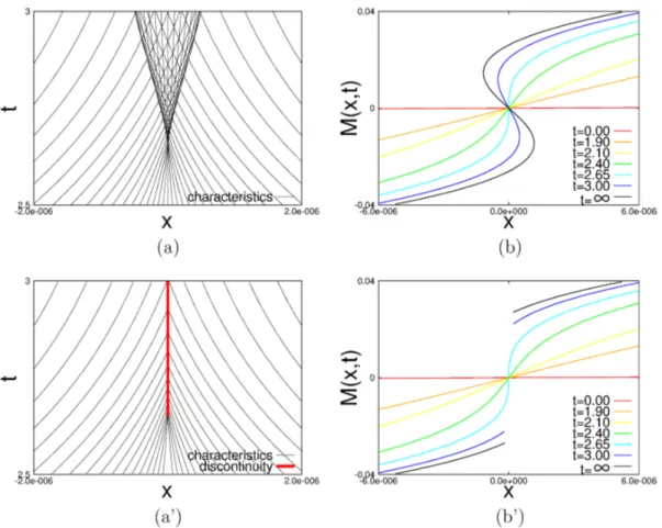
The numerical solution of the characteristic curves and the setof local strong solutions

$M(x;t)$ _{constructed by them are shown in Fig. 2 (a), (b). The characteristic curves} $\overline{x}(t)$

can be regarded

as

the contour lines of $lII(x;t)$ _{because the right-hand side of Eq. (12)}

vanishes. After $t_{c}$, the contour lines

cross

each other, and thenthe set ofthe local strong

solutions $\Lambda\ell(x;t)$ has a folding structure. Thus the set, which has the multi values, can

no

longer be the global solution of the PDE (8). On the other hand, the weak solution

can be constructed by the patchwork of the local strong solutions, which is determined

using the RH condition (10).

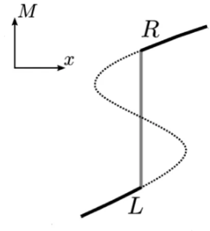
Figure 1: Equal (vanishing)

area

rule.

For the practicalpurpose, we here convert theRH condition to ageometric one

equiv-alent to itas follows. The totalderivatives of left and right limits of the fermion potential

$V_{W}(x;t)$ on thejump position $S(t)$ is given by

$dV_{W}^{L,R}= \frac{\partial V}{\partial x}|_{L,R}dS+\frac{\partial V}{\partialt}|_{L,R}dt$

$=M|_{L,R}dS-F|_{L,R}dt$, (16)

The difference between the left and right limits of Eq. (16) vanishes because of the RH

condition: $d(V_{W}^{L}-V_{W}^{R})=0$. Since

no

singular point doesn’t exist at the initial condition,

the fermion potential is entirely continuous

even

at the jump position $S(t)$:

$V_{W}^{L}=V_{W}^{R}$. (17)

Next, we integrate the set of the local strong solutions of $lII(x;t)$ as follows:

$\int_{L}^{R}Mdx=\int_{L}^{R}\frac{\partial V_{W}}{\partial x}dx$

$=V_{W}^{R}-V_{W}^{L}$

Thus the jump position

can

geometrically be determined by the equal (vanishing)

area

rule (Fig. 1). In Fig. 2,

we

now

show the weak solution constructed from the local strong

solutions at $G_{0}=1.005G_{c}$ using the equal

area

rule. The jump appears at the origin

after the critical scale $t_{c}$. The uniqueness of

our

weak solution is proved because of the

entropy condition, which guarantees the uniqueness of weak solution when the selected

characteristic curves fill the x-t plane [9]

as

shown in Fig. 2(a’).

(a) (b)

(a’) (b’)

Figure 2: (a) Characteristics. (b) Set of local strong solutions of

mass

function given by

the characteristics. (a’) Characteristics selected by the RH condition andjump

(discontinuity). (b’) Weak solution of

mass

function. The jump position obey

the equal (vanishing) area rule.

4

Bare

mass

In the previous section,

we

have obtained the $S\chi SB$ weak solution with a finite jump at

the origin. However the physical

mass

of quark

as

anorder parameter of chiral symmetry

cannot be determined since the mass function at the origin is not defined. To define the

order parameter,

we

introduce the bare mass term $m_{0}\overline{\psi}\psi$, which explicitly breaks the

chiral symmetry, to the Lagrangian(1). The bare

mass

term modifies the initial condition

of the PDE(8): $M(x;t=0)=G_{0}x+m_{0}$. Then, because ofthe translation invariance of

follows:

$M(x;t, m_{0})=M(x+m_{0}/G;t, m_{0}=0)$. (19)

Then the mass function at the origin is well defined because the jump appears not at the

origin but at $x=-m_{0}/G$. Thus, taking the limit $m_{0}arrow+0$ (called the chiral limit), we

can define the $t$-dependent effective mass _{$M_{phs}(t)$}

as

theorder parameter:

$M_{phys}(t)= \lim_{m0arrow+0}M(x;t, m_{0})|_{x=0}$ . (20)

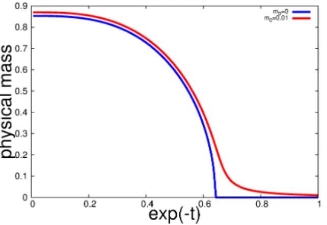
Fig.3 shows the RG evolutions of the physical

masses

in the chiral limit and at the

non-zero bare

mass.1

The physical

mass

in the chiral limit shows the second order phase

transition due to the singular behavior of the

mass

function at the origin, while the

physical

mass

at $m_{0}\neq 0$ shows the

cross over.

The

reader may think that the

weak-solution method is not necessary if $m_{0}\neq 0$. However global methods, such

as

the weak

solution, is needed at the small bare mass compared to the physical mass since the

mass

function has the jump

near

the origin. Actually, Ref. [2] shows that the Taylor expansion

to solve the PDE7 does not work at the small bare mass.

Figure 3: RG evolution of the physical masses in $m_{0}arrow 0$ and $m_{0}=$ O. The NPRG

equation given by Eq. (21) $(\mu=0, G=1.7G_{c})$ is used for evaluating the

physical

mass

to compare the result at finite chemical potential $\mu\neq 0.$

5

First

order phase

transition

at

finite chemical

po-tential

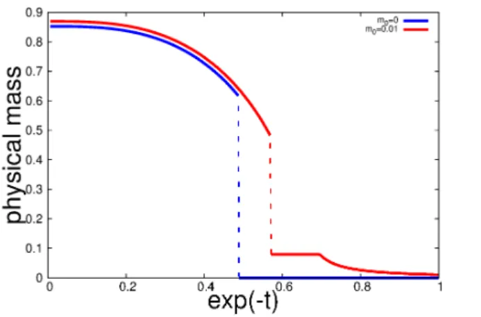
Let us consider the first order phase transition at finite chemical potential $(\mu\neq 0)$ using

the weak-solution method. The first order phase transition is more non-trivial than the

second order phase transition because the RG evolution of the physical mass has a finite

jump

even

at $m_{0}\neq 0$ (as shownin Fig. 4). Moreover the non-uniqueness of weak solution

is associatedwiththefact that theeffectivepotential, which is non-convex, has the

Figure 4: RG evolutions of the physical mass at finite density.

atfinite chemical potentialisuniquely determined, andtheeffectivepotential constructed

by the weak solution is automatically “convexised” with only the

one

correct minimum.

Thechemical potential$\mu$isintroduced by adding the term

$\mu\overline{\psi}\gamma_{0}\psi$

tothe Lagrangian (1).

For thesimpleNPRGequation, weusethespacialmomentumcutoff: $\sum_{i=1}^{3}p_{i}^{2}\leq\Lambda^{2}$. Then

the right-hand side of Eq. (8) changes $to^{2}$

$-F(x;t)= \frac{\Lambda^{3}}{\pi^{2}}[\sqrt{\Lambda^{2}+M^{2}}+(\mu-\sqrt{\Lambda^{2}+M^{2}})\cdot\Theta(\mu-\sqrt{\Lambda^{2}+M^{2}})]$ _{, (21)}

where $\Theta(x)$ is the Heaviside stepfunction. The characteristic curve is consequently given

by the following ODE:

$\frac{d\overline{x}(t)}{dt_{ノ}}=-\frac{\Lambda^{3}M}{\pi^{2}\sqrt{\Lambda^{2}+M^{2}}}\Theta(\sqrt{\Lambda^{2}+M^{2}}-\mu)$ . (22)

In Fig. 5, we show thecharacteristic curves and those selected by the RH condition which

are evaluated at $m_{0}=0,$ $\mu=0.7$. and $G_{0}=1.7G_{c}$. Fig. 5 (b) shows the uniqueness of

our weak solution because the entropycondition is satisfied. Fig. 6 (a), (b) show the weak

solutions of the

mass

function and the fermion potential at $m_{0}=0.01\Lambda_{0}$. These figures

shows that intheRG procedure the two jumps simultaneouslyappear,

move

toward each

other, and finally merge into one. Thus the RG evolution of the physical mass shows the

first order phase transition as shown in Fig.4.

In the rest of this section, we discuss the convexity of the Legendre effectivepotential

constructed by the weak solution. At first, we define the free energy $W(j;t)$ by

intro-ducing the external

source

for the chiral condensates $\langle\overline{\psi}\psi\rangle$: its

source

term $j\overline{\psi}\psi$, which

is distinguished from the

mass

term, is added to the Lagrangian(1). Then the initial condition of the fermion potential is

$V_{W}(x;t=0,j)=m_{0}x+ \frac{G_{0}}{2}x^{2}+jx$_{. (23)}

lIn thereal world thebare mass has thenon-zero value given bythe Higgs mechanism.

(a) (b)

Figure 5: (a) Characteristics. (b) Characteristics selected by theRH condition andjump

(discontinuity).

Now the free energy and the chiral condensates are given by

$W(j;t)=V_{W}(x=0;t,j)$, (24)

$\phi(j;t)\equiv\langle\overline{\psi}\psi\rangle_{j}=\frac{\partial W(j;t)}{\partial j}$, (25)

respectively. Weeventually define the Legendreeffectivepotentialof the chiral condensate

as follows:

$V_{L}(\phi;t)=j\phi(j;t)-W(j;t)$, (26)

where $\partial V_{L}/\partial\phi=j$ is satisfied.

As

seen inthe previous section, because ofthe translation invariance ofthePDEwith

respect to $x$, the fermion potential at $j\neq 0$ is given by the one at _$j=0$:

$V_{W}(x;t, j)=V_{W}(x+j/G_{0};t,j=0)- \frac{m_{0}j}{G_{0}}-\frac{j^{2}}{2G_{0}}$_{, (27)}

Thus the free energy and the chiral condensates are given by the quantities at $j=0$

as

follows:

$W(j;t)=V_{W}(x=0;t,j)=V_{W}(j/G_{0};t,j=0)- \frac{m_{0}j}{G_{0}}-\frac{j^{2}}{2G_{0}}$_{, (28)}

$\phi(j;t)=\frac{1}{G_{0}}[M(j/G_{0};t, j=0)-m_{0}-j]$ . (29)

Since

the set of local strong solutions of the mass function $M(j/G_{0};t,j=0)$ is

multi-valued, that of $\phi(j;t)$ is so. Obeying the equal area rule, the weak solution of $\phi(j;t)$ is

then constructed from its local strong solutions

as

well

as

the

mass

function.

The set of strong solutions of $V_{L}(\phi;t)$ is not convex and has multi local minima

as

shown Fig.6(c). On the other hand, we can prove that its weak solution is the

strongsolution

as

follows. Because of the continuityof the fermionpotential(17), the free

energy is also continuous at the jump position $j_{s}$ of the

mass

function $M(j/G_{0};t,j=0)$:

$W^{L}-W^{R}=V_{W}^{L}-V_{W}^{R}=0$. (30)

Using this continuity of the free energy and Eq. (26), we obtain

$\frac{V_{L}^{L}-V_{L}^{R}}{\phi^{L}-\phi^{R}}=j_{s}$, (31)

which

means

that the line connecting the Legendre effective potential $V_{L}(\phi;t)$ at the two

positions $\phi^{L},$ $\phi^{R}$ agrees with the envelope since $\partial V_{L}/\partial\phi|_{L,R}=j_{S}$. Thus theweak solution

of the effective potential is automatically convexised and has the correct minimum which

agrees with the global minimum of the local strong solutions as shown in Fig.6.

6

Summary

In this article,

we

have introduced the weak solution to define the singular $S\chi SB$ solution

of NPRG equation that can predict physical quantities such

as

the physical quark

mass

and the chiral condensates. The weak solution satisfies the integral-form (weak) of the

PDE. Specifically

we

haveevaluated the weak solutionofthe large-N

NPRG

equationfor

the

mass

function whichis the first derivative of the fermionpotential with respect to the

scalar bilinear-fermion field $\overline{\psi}\psi.$

We have constructed the weak solution by the method of characteristics. The set of

local strongsolutions given by the characteristics is multi-valued and thus

no

longeris the

global solution of the PDE. The weak solution can geometrically be constructed by the

patchwork ofthe local strong solutions using the equal

area

rule, which is derived by the

Rankine-Hugoniot condition. The uniqueness of the weak solution has been guaranteed

by the entropy condition. Then

we

have obtained the $S\chi SB$ weak solution of the

mass

function with

a

finitejump at the origin.

The method of weak solution has also been applied to the first order phase transition

at finite chemical potential. We have shown that in the RG procedure two jump appear

simultaneously,

move

toward each other, and finally merge into one. This RG evolution

is nothing but the first order phase transition. Finally

we

have discussed the convexity

ofthe Legendre effective potential of the chiral condensates which is constructed by the

weak solution of the fermion potential. The weaksolutionofthe effectivepotential, which

shows the first orderphase transition in theRG procedure, is automatically “

convexised”

with only one correct minimum, while the effective potential obtained by the mean-field

analysis has the multi local minima.

Acknowledgements

The authors greatly appreciate helpful lectures by Prof. Akitaka Matsumura who told

us

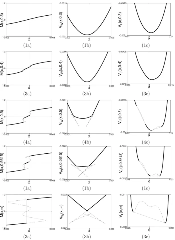
(1a) (1b) (1c) (3a) (3b) (3c) $00291$ $000365$ $\hat{tf)}$ $\overline{\eta.}$ $>^{\geq}\vee o_{-}x$ : $>^{\lrcorner}\vee\hat{\Leftrightarrow}0$ $\backslash$ $C$ $002*001$ $g$ $0001$ $000 \int_{02}$ $\theta$ 002 (1a) (1b) (1c) (3a) (3b) (3c)

Figure 6: RG evolution of physical quantities by weak solution with

non-zero

bare

mass

$(G_{0}=1.7G_{c}, m_{0}=0.01\Lambda_{0}, \mu=0.7, t=0.3,0.4,0.5,0.5615, \infty)$. (a) Mass

function. (b) Fermion potential. (c) Legendre effective potential. The thick

solid lines denote the weak solution, and the dashed linesdenotethelocalstrong

solutions dropped by the equal

area

rule. The thin solid line in (c) denotes the

References

[1] K.-I. Aoki, K. Takagi, H. Terao, and M. Tomoyose, Prog.Theor.Phys. 103,

815

(2000), hep-th/0002038.

[2] K.-I. Aoki and D. Sato, PTEP 2013, 043B04 (2013),

1212.0063.

[3] K.-I. Aoki, (1996), hep-ph/9706204.

[4] K.-I. Aoki, Prog.Theor.Phys.Suppl. 131, 129 (1998).

[5] K.-I. Aoki, K. Morikawa, J.-I. Sumi, H. Terao, and M. Tomoyose, Phys.Rev. D61,

045008

(2000), hep-th/9908043.

[6] H. Gies and C. Wetterich, Phys.Rev. D65, 065001 (2002), hep-th/0107221.

[7] K.-I. Aoki, Int.J.Mod.Phys. B14,

1249

(2000).

[8] J. Braun, J.Phys. G39,

033001

(2012),

1108.4449.

[9] L. C. Evans, Partial

_{Differential}

Equations, 2nd Edition (Amer Mathematical

Soci-ety, 2010).

[10] K.-I. Aoki, S.-I. Kumamoto, and D. Sato, in preparation (2014).

[11] F. J. Wegner and A. Houghton, Phys.Rev. A8,

401

(1973).