The mechanistic basis of population models with various types of competition (Theory of Biomathematics and its Applications V)

The

mechanistic basis of

population

models with

various

types of competition

Masahiro Anazawa

Department

_of

Environmental

_Information

Engineering, Tohoku Institute

_of

Technology

1

Introduction

The population dynamics ofsinglespecieswith seasonalreproduction

are

often modeled

using difference equations $x_{t+1}=f(x_{t})$, in which the expected population size $x_{t+1}$ in generation $t+1$ is expressed

as

a

function of the population size $x_{t}$ in generation $t$.

In most studies, these models have been introduced $a\epsilon$ top-down, phenomenological

models without sufficient mechanistic basis

on

individual level. Deriving population

modelsfrom processes

on

individual level is

an

effective

way torevel possiblemechanisms

that underlie these models. Recently, extending Royama’s method[l] in deriving the

Ricker model from local competition between individuals, first-principles derivations

of various discrete-time population models have been presented employing site-based

frameworks[2, 3, 4, 5]. Major population models derived in [4, 5] are presented in

Tabel 1. These models

were

derived by assuming that the competition type between

individuals

was

either scramble

or

contest.

In this article,

we

present

a

derivation of

a

new

population model that incorporates these population models

as

special cases, byconsidering partitioningof

resource

between

individuals[6]. Themodel derived has twoparametersrelating tothe type of competition

and spatial aggregation of individuals respectively, and it provides

a

unified view about

relationships between various population models in terms of the two parameters.

Table 1: Major population models derived in

site-based frameworks.

type distr. model see Eq. name

$R$ $k_{1}x_{t}\exp(-k_{2}x_{t})$ (15) Ricker scramble $N$ $k_{1}x_{t}/(1+k_{2}x_{t})^{d}$ (12) Hassell $R$ _{$k_{1}[1-\exp(-k_{2}x_{t})]$} (16) Skellam contest $N$ $k_{1}[1-(1+k_{2}x_{t})^{-d}]$ (13) Br\"annstrom-Sumpter[4] $N$ $k_{1}x_{t}/(1+k_{2}x_{t})$ (19) Beverton-Holt

In the columm ‘distr.’, assumed types of distributionofindividuals overtheresource

sitesare specified. $R$, random (Poisson) distribution; $N$, negative binomial

distribu-tion.

2

Site-based

framework

This study is based

on a

site-based framework[2, 3, 4, 5], which we will describe in the following.

Consider

a

habitat consisting of $n$

resource

sites

over

which $x_{t}$ individuals

of single species

are

distributed in generation $t$

.

We

assume

that the expected number

of offspring emerging from each site depends only

on

the number of the individuals

at

the

site.

We

let $\phi(k)$ be the expected number of offspring emerging

from

a

site

containing $k$ individuals. This function is referred to

as

the interaction function. All

individuals emerging from all the sites disperse and

are

distributed

over

the

resource

sites again. These individuals form

a

population in generation $t+1$

.

The expected

number of individuals in generation $t+1$ is written

as

$x_{t+1}=n \sum_{k=1}^{\infty}p_{k}\phi(k)$, (1) where$p_{k}$ denotes theprobabilityof finding$k$ individuals at agiven site. The distribution $p_{k}$ is a function of$x_{t}$ and $n$. Eq. (1) connects the density dependence

on a

scale ofsite

(patch), $\phi(k)$, with the whole population dynamics. Choosing $p_{k}$ and $\phi(k)$ determines

the explicit form of the discrete-time population model $x_{t+1}=f(x_{t})$ for the whole

population. According to scale transition theory[7], population dynamics

on

the

whole

population scale are, in general, determined by interactions between spatial variations

and nonlinear dynamics

on

the scale of local populations.

As for the distribution $p_{k}$, we

assume

the following negative binomial distribution

with expectation $x_{t}/n$:

$p_{k}= \frac{\Gamma(k+\lambda)}{\Gamma(\lambda)\Gamma(k+1)}(\frac{x_{t}}{\lambda n})^{k}(1+\frac{x_{t}}{\lambda n})^{-k-\lambda}$, (2)

which corresponds to

a

situation in which individuals are forming some clusters. Here,

$\lambda$ is a positive parameter, where

$1/\lambda$ represents the degree of spatial aggregation of

individuals. In the limit

as

$\lambdaarrow\infty$, Eq. (2) becomes

a

Poisson distribution with

expectation $x_{t}/n$, which corresponds to a situation in which individuals

are

distributed

completely at random.

As

for the interaction function,

$\phi(k)=\{\begin{array}{l}1 for k=1,(3)0 for otherwise,\end{array}$

was

used in [4] forscramble competition, and

$\phi(k)=\{\begin{array}{l}1 for k\geq 1,(4)0 for otherwise,\end{array}$

for contest competition. Eq. (3) describes

a

situation in which each site

can

maintain

only

one

individual: iftwo

or

more

individuals share

a

site, then they fail to reproduce.

On

the other hand, Eq. (4) describes

a

situation in which

one

successful individual gets

all of the

resource

it requires to reproduce and the others in the

same

site cannot

repro-duce.

A

more

general interaction function

was

used in [5] for each type of competition.

3

A model for intermediate competition

3.1

Derivation

from

resource

partitioning

As

a new

interaction function which exhibitscompetitionintermediate between scramble

and contest, andincorporates the interactionfunctions described in the preceding section

as

special cases, we propose the following function:

$\phi(k)=b\frac{\hat{c}^{k}-c^{k}}{\hat{c}-c}$, (5)

where $0<c<\hat{c}<1$

.

_{We refer to the competition type corresponding to this function}

as

‘intermediate competition’. In the following,

we

present

a

derivation ofEq. (5) from

the viewpoint of

resource

partitioning. We suppose that each individual has

a

minimum

sufficient

resource

requirement $s$ tosurvive and reproduce; if

an

individualcannotobtain

the amount $s$ofresource, itfails toreproduce. Weconsider

resource

partitioningin

a

site

which contains $k$ individuals and

an

amount $R$ of

resource.

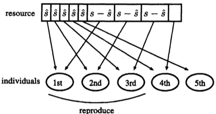
As an intermediate between

ideal scramble and ideal contest cases, combining two kinds ofresource partitioning,

we

assume

the following way of partitioning: first,

an

amount $\hat{s}$ is equally

given to all the

individuals in the site, and then the remaining

resource

inthe site ispartitioned in order

of their competitive abilities (seeFigure 1). If$R- sk<(s-\hat{s})m$, the m-thindividual in

the site cannot obtain the amount $s$ of

resource

necessary

for reproduction, and fails to

reproduce. Letting $\phi_{m}(k)$ be the expected number of offspring reproduced by the m-th individual in

a

given site with $k$ individuals, we can write _{$\phi_{m}(k)$}

as

$\phi_{m}(k)=b’\int_{sk+(e-\hat{s})m}^{\infty}q(R)dR$, (6)

where $b’$ is

a

positive constant, and _$q(R)$ denotes the probability density that

a

given

site has

an

amount $R$ of

resource.

Here,

we

assume

that _$q(R)$ is given by

an

exponential

distribution

$q(R)= \frac{1}{R}e^{-R/\overline{R}}$, (7)

where$\overline{R}$ denotesthe expected value of

$R$

.

The interactionfunction$\phi(k)$

can

be obtained by adding up the contributions from all the individuals in the site

as

$\phi(k)=\sum_{m=1}^{k}\phi_{m}(k)$

.

(8)

Combining Eqs. (6), (7) and (8), and performing the summation above give the

inter-action function (5) under the following relations: $b=b’c,$ $c=e^{-\epsilon/\overline{R}}$and $\hat{c}=e^{-\hat{s}/\overline{R}}$

.

The

derivation above shows that it is possible to interpret Eq. (5)

as

a consequence ofthe

exponential

distribution

(7) and the way of

resource

partitioning which is intermediate

between exactly equal partitioning and that in order of competitive ability.

We next derive a population model corresponding to the interaction function (5) for

the intermediatecompetition. Substituting Eqs. (5) and (2) intoEq. (1), and performing

the summation give the following population model:

reproduce

Figure 1: $m_{ustration}$ _{ofthe way of}resource _{partitioning in} a _{site for the}

interme-diate competition. At first, each individual equally takes an amount $\hat{s}$ of resource,

and then tries to take an amount $s-\hat{s}$ ofresource from the remaining resource in

order ofcompetitive ability. Only the individuals that are ableto get the amount $s$

of

resouroe

intotal reproduce.

where

$\hat{x}_{t}=(1-c)x_{t}$, (10)

$\beta=\frac{1-\hat{c}}{1-c}=\frac{1-e^{-\hat{s}/R}}{1-e^{-\epsilon/\overline{R}}}$

.

(11)

Eqs. (9) and (10) show that reproduction

curves

$x_{t+1}=f(x_{t})$ for variousvalues of$c$

are

all similar ifthe otherparameters are fixed. As for the parameter $\beta$, models with $\beta=0$

correspond to the

case

of ideal contest competition, and models with $\beta=1$ to that of

ideal scramble competition. Thus, $\beta$

can

be regarded

as

the degree of deviation from

ideal contest competition.

3.2

Relationships

between

vaiious

population

models

The population model derived above, Eq. (9), allows

us

to understand in

a

uni-fied

way relationships between various population models derived

so

far in site-based

frameworks[4, 5] in terms of two parameters $\lambda$ and $\beta$. Figure 2 illustrates these

re-lationships in a coordinate system of $1/\lambda$ and $\beta$

.

Here, $1/\lambda$ represents the degree of

aggregation of individuals, and $\beta$ the degree of deviation from ideal contest

competi-tion.

As we

describe in the following, various population models

can

be regarded

as

certain limit

cases

ofEq. (9). The limit

as

$\betaarrow 1(\hat{c}arrow c)$ corresponds to ideal scramble competition, and in this limit, Eq. (9) becomes

$\hat{x}_{t+1}=b\hat{x}_{t}(1+\frac{\hat{x}_{t}}{\lambda n})^{-\lambda-1}$, (12)

which is theHassell model. On the other hand, the limit

as

$\betaarrow 0(\hat{c}arrow 1)$ corresponds

to ideal

contest

competition, and in this limit, Eq. (9) becomes

Figure 2: Relationships between various population models

are

described in a

$(1/\lambda,\beta)$ coordinate system. Here, $1/\lambda$ indicates the degree ofspatial aggregation

ofindividuals, and$\beta$ the degree ofdeviation from ideal contest competition.

Vari-ous models

can

be regarded as limit cases of the model of intermediate competition

type.

which is the Br\"annstr\"om-Sumpter model[4].

We next consider the limit

as

$\lambdaarrow\infty$. This limit corresponds to the

case

in which

individuals

are

distributed completely at random

over

resource

sites according to

a

Poisson distribution. In this limit, Eq. (9) becomes

$\hat{x}_{t+1}=\frac{nb}{1-\beta}(e^{-\beta\hat{x}_{t}/n}-e^{-\hat{x}z/n})$

.

(14)

Furthermore, taking the limit

as

$\betaarrow 1(\hat{c}arrow c)$ in Eq. (14) yields

$\hat{x}_{t+1}=b\hat{x}_{t}e^{-\hat{x}_{t}/n}$, (15)

which is the Ricker model.

On

the other hand, taking the limit

as

$\betaarrow 0(\hat{c}arrow 1)$ in

Eq. (14) yields

$\hat{x}_{t+1}=nb(1-e^{-f_{t}/n})$, (16)

which is the Skellam model.

We next

consider

the

case

of $\lambda=1$, in which the distribution (2) becomes the

geometrical distribution $p_{k}=(x_{t}/k)^{k}(1+x_{t}/n)^{-(1+k)}$

.

In this case, Eq. (9) takes the

form of

Taking the limit

as

$\betaarrow 1(\hat{c}arrow c)$ further in Eq. (17) gives

$\hat{x}_{t+1}=\frac{b\hat{x}_{t}}{(1+\hat{x}_{t}/n)^{2}}$, (18)

which is the Hassell model.

On

the other hand, taking the limit

as

$\betaarrow 0(\hat{c}arrow 1)$ in

Eq. (17) gives

$\hat{x}_{t+1}=\frac{b\hat{x}_{t}}{1+\hat{x}_{t}/n}$, (19)

which is the Beverton-Holt model. Aswe have shown above, various populationmodels

can

beobtained from the model (9) in various limits with respect tothe two parameters

$\lambda$ and $\beta$

.

4

Conclusions

Byconsideringpartitioningof

resource

between individualsin each site, anddistribution

of individuals

over

the sites,

we

have derived a

new

discrete-time population model for

a

competition type intermediate between scramble and contest. The derived model in-corporates various population models

as

limit

cases

in terms of two parameters relating

to the type of competition and the degree of spatial aggregation of individuals

respec-tively. In this sense, the model provides a unified view about relationships between

these population models interms of the two parameters.

References

[1] T. Royama. Analytical population dynamics. Chapman&Hall, London, 1992.

[2] D. J. T. Sumpter and D.

S.

Broomhead. Relating

individual

behaviour

to

population dynamics. Proc. R. Soc. B, 268:925-932, 2001.

[3] A. Johanssonand D. J. T. Sumpter. From local interactions to population dynamics

in site-based models of ecology. Theor. Popul. Biol., 64:497-517,

2003.

[4]

A.

Br\"annstrom and D. J. T. Sumpter. The role of competition and clustering in

population dynamics. Proc. R. Soc. London B, 272:2065-2072,

2005.

[5] M

Anazawa.

Bottom-up derivationofdiscrete-time population modelswith the Allee

effect.

Theo

r.

Popul. Biol., 75:56-67,

2009.

[6] M

Anazawa.

The mechanistic basis of discrete-time population models: the role of

resource

partitioning and spatial aggregation. Theor. Popul. Biol., in press.

[7] P. Chesson. Making

sense

of spatial models in ecology. In J. Bascompte and

R. V. Sole, editors, Modeling Spatiotemporal Dynamics in Ecology,

pages 151-166.