平面内の曲線の運動 (現象の数理解析へ向けた非線形発展方程式とその周辺)

平面内の曲線の運動1)

On

motion of

curves

in

the

plane

宮崎大学・工学部 矢崎 成俊 (Shigetoshi Yazaki)

Faculty ofEngineering, University ofMiyazaki2) Contents.

1. Introduction

2. Curvature adjusted tangential velocity 3. Image segmentation

4. Hele-Shaw flow in a time-dependent gap

1 Introduction

In this talk

we

study evolution of

a

family of closed smooth plane

curves:

$x$ : $[0,1]\cross[0, T)arrow\Gamma(t)=\{x(u, t)\in \mathbb{R}^{2};u\in[0,1]\subset \mathbb{R}/\mathbb{Z}\}$,

starting from a given initial curve $\Gamma(0)=\Gamma_{0}$, and driven by the evolution law:

$\partial_{t}x=\alpha t+\beta n$,

where $t=\partial_{u}x/|\partial_{u}x|$ is the unit tangent vector, and $n$ is the unit outward normal vector

which satisfies $\det(n, t)=1$. Here and hereafter, wedenote $\partial_{\xi}F=\partial F/\partial\xi$ and $|a|=\sqrt{a}a$

where $a.b$ is Euclidean inner product between vectors $a$ and $b$

.

The solution

curves are

immersed

or

embedded such that $|\partial_{u}x|>0$ holds.

We remark that the tangent velocity $\alpha$ has no effect of shape ofsolution

curves

and

affect only parametrization. Therefore, the shape of solution

curves are

determined by

the normal velocity $\beta$, and

a

nontrivial tangent velocity $\alpha$ will be chosen depending

on

the purpose.

The normal velocity $\beta$ may depend

on

many factors, which

are

arising in various

applied fields like e.g. the material sciences, dynamics of phase boundaries in

thermome-chanics, computationalgeometry, image processing and computer vision, fluid dynamics,

the field of ice and snow crystal, etc. For the comprehensive overview ofapplications we

refer the book by Sethian [14]. According to the book, $\beta$

can

be written

as:

$\beta=\beta(\mathcal{L};\mathcal{G};\mathcal{I})$,

where

1$)$

Manuscript for “現象の数理解析に向けた非線形発展方程式とその周辺”, October 13 –15, 2010 at

RIMS, Kyoto University. The author ispartiallysupported byGrant-in-Aid forEncouragement ofYoung

Scientists (No. 21740079).

$\bullet$ $\mathcal{L}ocal$ properties are those determined by local geometric information of$\Gamma$, such as

the curvature $k$ and the normal

or

the tangential direction.

$\bullet$ $\mathcal{G}lobal$ properties of$\Gamma$ arethose that depend on the shape and the position of$\Gamma$, such

as

the position vector $x\in\Gamma$, the length of $\Gamma$, and the integrals along $\Gamma$ associated

PDEs, etc.

$\bullet$ $\mathcal{I}ndependent$ properties are those that are independent of the shape of$\Gamma$, such as

an underlying fluid velocity, etc.

Here $k$ is the curvature in the direction

$-n$, which is defined from $\partial_{s}t=-kn,$ $\partial_{s}n=kt$,

and described

as

$k=\det(\partial_{s}x, \partial_{ss}x)$, and $\partial_{s}x=t$ is the unit tangent vector. Here and

hereafter,

we

denote $\partial_{\xi\xi}F=\partial(\partial_{\xi}F)/\partial\xi$. Note that $\partial_{s}$ is not partial differentiation. It

means

the operator $\partial_{s}F(u, t)=g(u, t)^{-1}\partial_{u}F(u, t)$, where$g(u, t)=|\partial_{u}x(u, t)|>0$ is called

the local length and $s$ is the

arc

length parameter determined from $ds=g(u, t)du$.

In this note, we will focuson the utilization of a nontrivial tangential velocity $\alpha$, and

will mention on two applications in the

case

$\beta=\beta(\mathcal{L};\mathcal{G};\mathcal{I})$: one is image segmentation

with $\mathcal{L}(k, n);\mathcal{G}(x)$ or $\mathcal{L}(k);\mathcal{G}(x)_{)}\mathcal{I}(const.)$, and the other

one

is numerical computation

of Hele-Shaw flow in a time-dependent gap with $\mathcal{G}$(integral of a PDE).

2 Curvature adjusted tangential velocity

As mentioned in the previous section, the tangential velocity functional $\alpha$ has

no

effect

of the shape of evolving curves [5, Proposition 2.4], and the shape is determined by the

value of the normal velocity $\beta$ only. Hence the simplest setting $\alpha\equiv 0$ can be chosen.

Dziuk [4] studied a numerical scheme for $\beta=-k$ in this

case.

In the

case

general $\beta$,

however, such a choice of$\alpha$ may lead to various numerical instabilities caused by either

undesirable concentration and$/or$extreme dispersion of numerical grid points. Therefore,

to obtain stable numerical computation, several choices ofa nontrivial tangential velocity

have been emphasized and developed by many authors. We will present a brief review of

development of nontrivial tangential velocities.

Kimura [7, 8] proposed auniform redistribution scheme in the

case

$\beta=-k$ by using

a

special choice of $\alpha$ which satisfies discretization of an average condition and the uniform

distribution condition:

(U) $r(u, t)= \frac{g(u,t)}{L(\Gamma(t))}\equiv 1$ $(\forall u)$.

Hou, _{Lowengrub and Shelley [6] utilized condition (U) directly (especially for}$\beta=-k$)

starting from $r(u, 0)\equiv 1$, and derived

which

comes

from

$\partial_{t}r=\frac{g}{L}(\partial_{s}\alpha+k\beta-\langle k\beta\rangle)\equiv 0$ $(\forall u)$.

It

was

proposed independently by Mikula and

\v{S}ev\v{c}ovi\v{c}

[10]. In [6, Appendix 2], Hou et

al. also pointed out generalization of (2.1)

as

follows:

$\frac{\partial_{s}(\varphi(k)\alpha)}{\varphi(k)}=\frac{\langle f\rangle}{\langle\varphi(k)\rangle}-\frac{f}{\varphi(k)}$, $f=\varphi(k)k\beta-\varphi’(k)(\partial_{ss}\beta+k^{2}\beta)$ (2.2)

for

a

given function $\varphi$. If $\varphi\equiv 1$, then this is nothing but (2.1). (2.2) is derived from the

following calculation. Let a generalized relative local length be

$r_{\varphi}(u, t)=r(u, t) \frac{\varphi(k(u,t))}{\langle\varphi(k(\cdot,t))\rangle}$.

Then preserving condition $\partial_{t}r_{\varphi}(u, t)\equiv 0$ leads (2.2).

As mentioned above, in the paper [10] the authors arrived (2.1) in general frame work

of the so-called intrinsic heat equation for $\beta=\beta(\theta, k)$, where $\theta$ is the angle of

$n$, i.e.,

$n=(\cos\theta, \sin\theta)$ and $t=(-\sin\theta, \cos\theta)$. This result

was

improvement of [9] in which

satisfactory results

were

obtained only in the

case

$\beta=\beta(k)$ being linear and sublinear

with respect to $k$. Afterthese results, in the series ofthepaper [11, 12, 13], theyproposed

method ofasymptotically uniform redistribution, i.e., derived

$\partial_{s}\alpha=\langle k\beta\rangle-k\beta+(r^{-1}-1)\omega(t)$ (2.3)

for quite general normalvelocity $\beta=\beta(x, \theta, k)$, where $\omega\in L_{loc}^{1}[0, T)$ is

a

relaxation

func-tion satisfying $\int_{0}^{T}\omega(t)dt=+\infty$

.

Their method succeeded and

was

applied to geodesic

curvature flows and image segmentation, etc.

Besides these uniform distribution method, under the so-called crystalline curvature

flow, grid points are distributed dense (resp. sparse)

on

the subarc where the absolute

value ofcurvatureis large (resp. small). Althoughthis redistribution is far from uniform,

numerical computation is quite stable. One of the

reason

is that polygonal

curves are

restricted in

an

admissible class. To apply the

essence

of crystalline curvature flow to a

generaldiscretization model of motion of smooth curves, thetangentialvelocity$\alpha=\partial_{s}\beta/k$

was

extracted, which is utilized in crystalline curvature flow equation implicitly [18].

The asymptotically uniform redistributionis quiteeffective and validfor wide

range

of

application. However, from approximation point ofview, unless solution

curve

isa circle,

thereis

no

reason

to take uniform redistribution. Hence the redistribution will be desired

in

a

way of taking into account the shape of evolution curves, i.e., depending

on

size of

curvatures. In the paper [15, 16], it is proposed that a method of redistribution which

takes into account the shapeoflimiting curve such

as

If $\varphi\equiv 1$, then this is nothing but (2.3), and if $\varphi=k$ and $\Gamma$ is convex, we have _{$\alpha=\partial_{s}\beta/k$}

in the

case

$\omega=0$

.

Therefore, this is a combination of method of asymptotic uniform

redistribution and the crystalline tangential velocity

as

mentioned above. Notice that

this method was applied to an image segmentation and nice results were confirmed [2].

To complete the overview of various tangential redistribution method we also mention

a

locally dependent tangential velocity. For the

case

$\beta=-k$ it

was

proposed by

Deckel-nick [3] who used $\alpha=-\partial_{u}(g^{-1})$

.

Then the evolution equation becomes

a

simple parabolic

PDE $\partial_{t}x=g^{-2}\partial_{u}^{2}x$.

As faras$3D$implementationoftangentialredistribution is concerned, in

a

recent paper

by Barrett, Garcke and N\"urnberg [1] the authors proposed and studied

a

new efficient

numerical scheme for evolution of surfaces driven bythe Laplacianof the

mean

curvature.

It turns out, that their numerical scheme has implicitly built in

a

uniform redistribution

tangential velocity vector.

3 Image segmentation

The gradient flow$\beta=-\gamma(x)k-\nabla\gamma(x).n$isutilizedfor image segmentation

as

follows. Let

an

image intensity function be $I:\mathbb{R}^{2}\supset\Omegaarrow[0,1]$. Here $I=0$ (resp. $I=1$) corresponds

to black (resp. white) color and $I\in(0,1)$ corresponds to gray colors. For simplicity,

we assume that our target figures are given in white color with black background. Then

the image outline or edge correspond to the region where $|\nabla I(x)|$ is quite large. Let

us

introduce an auxiliary function $\gamma(x)=f(|\nabla I(x)|)$ where $f$ is a smooth edge detector

function like e.g. $f(s)=1/(1+s^{2})$ _or $f(s)=e^{-s}$. Hence the solution

curve

$\Gamma(t)$ of

$\beta=-\gamma(x)k-\nabla\gamma(x).n$ makes the energy $E_{F}(\Gamma(t))$ smaller and smaller, in other words,

its

moves

toward the edge where $|\nabla I(x)|$ is large. This is a fundamental idea of image

segmentation, and it has developed to a sophisticated scheme [12, 13].

The following scheme is

more

simple [2]. In the following computations, the target

figure is given by adigital gray scale bitmap imagerepresented by integer values between

$0$ and255 on

some

prescribed pixels. The values $0$ and 255 correspond to black and white colors, respectively, whereas the values between $0$ and 255 correspond to gray colors.

Givenafigure,we can constructitsimage intensityfunction$I$ : $\mathbb{R}^{2}\supset\Omegaarrow\{0, \ldots, 255\}\subset$

$\mathbb{Z}$. Note that $I(x)$ is piecewise

constant in each pixel.

We consider the fiow $\beta=-k+F$ and define the forcing term $F(x)$

as

follows:

$F(x)=(F_{\max}-F_{\min}) \frac{I(x)}{255}-F_{\max}$ $(x\in\Omega)$,

where $F_{\max}>0$ corresponds to purely black color (background) and $F_{\min}<0$

corre-sponds to purely white color (the object to be segmented). Maximal and minimal values

curve can

attain. The choice of small values of $F$

causes

the finalshape to be

rounded or

the

curve

can

not

pass

through

narrow

gaps.

4 Hele-Shaw flow in

a

time-dependent

gap

The so-called Hele-Shaw flow is flow ofviscous liquid which is contained in the

narrow

gap

between two parallel plates, that is, in the Hele-Shaw cell. Figure 4.1 indicates the

Hele-Shaw

cell settled in the xyz-coordinate.

Figure4.1: Hele-Shaw cell

Let $b$be the gap between two parallel plates in the z-direction. In classical Hele-Shaw

experiments, $b$is fixedand taken around lmm. Shelley,Tianand Wlodarski [17] proposed

a

problem in the

case

where $b$ depends

on

the time $t$, i.e., the upper plate is being lifted

uniformly at a specific rate. They established the existence, uniqueness and regularity

ofsolutions in the

case

where the surface tension is

zero.

They also studied numerical

computation by

means

of

ODE

for the time discretization.

In this section, we will propose the boundary element method with

a

curvature

ad-justed tangential velocity.

We

assume

that there

are no

effect ofexternalforce like gravity in the Hele-Shaw cell

and the liquid is govemed by the Navier-Stokesequation:

$\frac{\partial v}{\partial t}+(v\cdot\nabla)v=-\frac{1}{\rho}\nabla p+\nu\Delta v$, (41)

where $\rho$ is density, $\nu$ is kinetic viscosity. Unknown functions

are

the pressure $p$ and the

velocity $v=(\begin{array}{l}uvw\end{array})$

.

In what follows,

we

will simplify this equations.

Firstly,

we

require the following.

(Al) the velocity of water is very slow, and the flow is stationary.

By this assumption, we operate $sorightarrow called$ Stokes approximation for stationary flow,

and theLHS of (4.1) is neglected:

$0=- \frac{1}{\rho}\nabla p+\frac{\mu}{\rho}\Delta v$, (4.2)

Secondly,

we

assume

that

(A2) the fluid does not

move

in the vertical direction, i.e.. $w=0$.

Then

we

have

$\nabla p=(\begin{array}{l}\partial_{x}p\partial_{y}p\partial_{z}p\end{array})=\mu\triangle v$, $v=(\begin{array}{l}uv0\end{array})$ .

From

this, $p=p(x, y, t)$

holds.

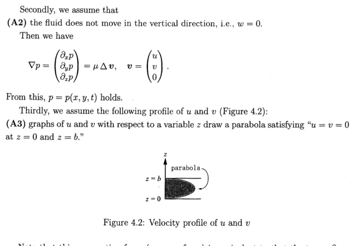
Thirdly,

we

assume

the following profile of$u$ and $v$ (Figure 4.2):

(A3) graphs of$u$and $v$ with respect to

a

variable $z$ draw aparabolasatisfying $u=v=0$

at $z=0$ and $z=b.$”

$z$

Figure 4.2: Velocity profile of$u$ and $v$

Note that this assumption for $u$ (same

as

for v) is equivalent to that the terms $\partial_{xx}u$

and $\partial_{yy}u$

are

negligible and the term $\partial_{zz}u$ is dominant in $\triangle u$. Then $u$ and $v$

can

be

expressed

as

$u(x, y, z, t)=\varphi(x, y, t)z(z-b)$, $v(x, y, z, t)=\psi(x, y, t)z(z-b)$

with functions $\varphi$ and $\psi$. Hence

we

have

$\partial_{x}p=\mu((\partial_{xx}\varphi+\partial_{yy}\varphi)z(z-b)+2\varphi)$, $\partial_{y}p=\mu((\partial_{xx}\psi+\partial_{yy}\psi)z(z-b)+2\psi)$ .

Since

the pressure is $p=p(x, y, t)$, we obtain

$\partial_{xx}\varphi+\partial_{yy}\varphi=0$, $\partial_{xx}\psi+\partial_{yy}\psi=0$.

Therefore from

$\partial_{xx}u+\partial_{yy}u=0$, $\partial_{xx}v+\partial_{yy}v=0$,

we

have

Fourthly,

we

require the following.

(A4) to take average of $u$ and $v$ in z-direction.

Then, the two dimensional average velocity vector is expressed by

a

gradient of

pres-sure:

$\overline{u}=\frac{1}{b}\int_{0}^{b}udz=\frac{\partial_{x}p}{2\mu b}[\frac{z^{3}}{3}-\frac{bz^{2}}{2}]_{0}^{b}=-\frac{b^{2}}{12\mu}\partial_{x}p)$ $\overline{v}=-\frac{b^{2}}{12\mu}\partial_{y}p$.

Hence the

average

velocityOf, $\overline{v}$and the

pressure

$p$

are

functions of three variables $(x, y, t)$,

respectively.

We

define the

two

dimensional

velocity such

as

$u=( \frac{\overline u}{v})$ .

Then

we

have

$u=- \frac{b^{2}}{12\mu}\nabla p$, $\nabla p=(\begin{array}{l}\partial_{x}p\partial_{y}p\end{array})$ ,

and from the incompressibility

$0= \frac{1}{b}\int_{0}^{b}divvdz=\frac{1}{b}\int_{0}^{b}(\partial_{x}u+\partial_{y}v+0)dz=\partial_{x}\overline{u}+\partial_{y}\overline{v}=-\frac{b^{2}}{12\mu}(\partial_{xx}p+\partial_{yy}p)$.

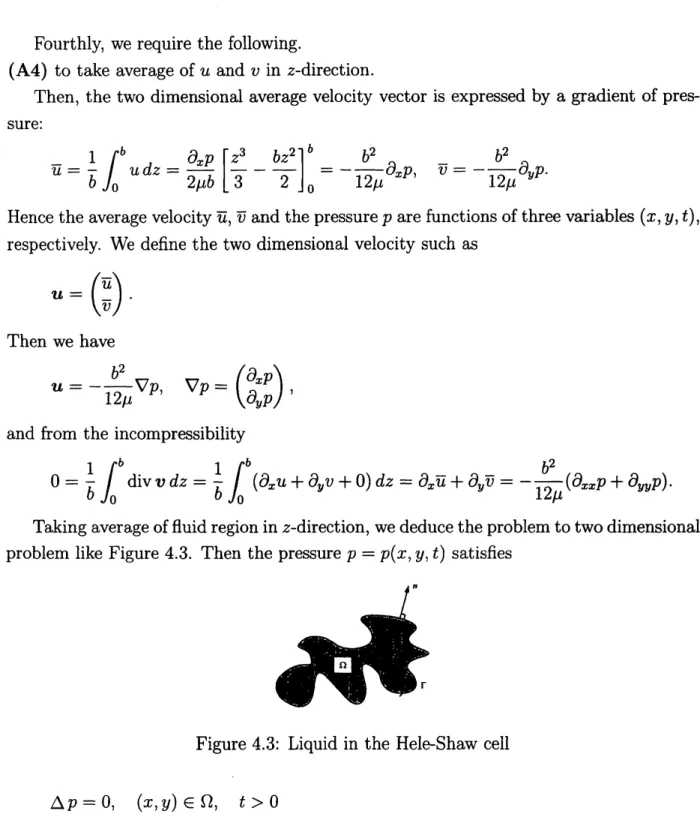
Takingaverage of fluidregion in z-direction,

we

deduce theproblemto twodimensional

problem like Figure

4.3.

Then the pressure $p=p(x, y, t)$ satisfies

Figure

4.3:

Liquid in

the

Hele-Shaw

cell

$\triangle p=0$, $(x, y)\in\Omega$, $t>0$

inthe interior of two dimensional fluidregion. Here wehavedefiedtwodimensional

Lapla-cian such

as

$\triangle p=\partial_{xx}p+\partial_{yy}p$

.

Since the boundary $\Gamma$

moves

with the fluid, deformation

velocity $\beta$ in the normal direction _$n$ of $\Gamma$ is given

as

$\beta=u\cdot n=-\frac{b^{2}}{12\mu}\frac{\partial p}{\partial n}$, $\frac{\partial p}{\partial n}=\nabla p\cdot n$.

Here the normal velocity of $\Gamma=\Gamma(t)$ is defined

as

Here

and hereafter,

we

denote $\dot{F}=\partial_{t}$F.

On the boundary $\Gamma$, we

use

the Laplace‘s

relation

$p-p_{*}=\tau k$, $\tau>0$

.

Here

$p_{*}$ is the atmospheric pressure and $\tau$ is

a

surface tension coefficient. Since $p_{*}$ is

a

constant,

we

have $\nabla(p-p_{*})=\nabla p$ and $\triangle(p-p_{*})=\triangle p$. Then

we can

assume

_{$p:=p-p_{*}$}

.

Consequently,

we

have the following classical Hele-Shaw problem:

(CHS) $\{\begin{array}{ll}\triangle p=0, (x, y)\in\Omega(t), t>0,p=\tau k, (x, y)\in\Gamma(t), t>0,\beta=-\frac{b^{2}}{12\mu}\frac{\partial p}{\partial n}, (x, y)\in\Gamma(t), t>0.\end{array}$

In our case, the gap $b$ is lifted uniformly at a specific rate. Then instead of (A2), we

assume

that

(A2)’ $w$ is

a

linear function with respect to $z$, i.e., $w=\eta(t)z+\xi(t)$.

At the bottom $z=0$, the fluid does not move. Then $\xi(t)=0$.

At

the top $z=b(t)$,

the fluid

moves

with the plate. Then $\eta(t)=\dot{b}(t)/b(t)$. Hence

we

have

$w= \frac{\dot{b}(t)}{b(t)}z$.

In this case, the pressure $p$ does not depend

on

$z$, since

$p_{z}=l^{l}\triangle w=0$.

We

can

discuss the

same

argument of$u$ and $v$

as

above, except the contribution from

incompressibility:

$0= \frac{1}{b(t)}\int_{0}^{b(t)}divvdz=\frac{1}{b(t)}\int_{0}^{b(t)}(u_{x}+v_{y}+w_{z})dz$

$= \overline{u}_{x}+\overline{v}_{y}+\frac{\dot{b}(t)}{b(t)}=-\frac{b(t)^{2}}{12\mu}(p_{xx}+p_{yy})+\frac{\dot{b}(t)}{b(t)}$.

Hence we

have

$\triangle p=12\mu\frac{\dot{b}(t)}{b(t)^{3}}$,

and the following Hele-Shaw problem in

a

time-dependent gap $b(t)$:

In the

case

the

plates

are

fixed,

then

$\dot{b}(t)=0$

and the above problem is

nothing

but the

classical

Hele-Shaw problem.

Now

we

will

arrange

the above problemby

dimensionalization

as

follows. The variables

$x,$ $y$ and $t$

are

scaled by a characteristic rate $l_{0}>0$ and $t_{0}>0$, respectively:

$\tilde{x}=\frac{x}{l_{0}}$, $\tilde{y}=\frac{y}{l_{0}}$, $\tilde{t}=\frac{t}{t_{0}}$.

Then the curvature $k$ and the normal velocity $\beta$

are

scaled by $\tilde{k}=k/k_{0},$ $k_{0}=l_{0}^{-1}$ and

$\tilde{\beta}=\beta/\beta_{0},$ _{$\beta_{0}=l_{0}/t_{0}$}, respectively. The pressure_$p$, the gap $b$and surface tension coefficient $\tau$

are

scaled by

a

characteristic rate$p_{0}>0,$ $b_{0}>0$ and $\tau_{0}>0$, respectively:

$\tilde{p}(\tilde{x},\tilde{y},$$t \gamma=\frac{p(x,y,t)}{p_{0}},$ $\tilde{b}(t\gamma=\frac{b(t)}{b_{0}},$ $\tilde{\tau}=\frac{\tau}{\tau_{0}}$.

If

we

take

$p_{0}= \frac{12\mu l_{0}^{2}}{b_{0}^{2}t_{0}}$, $\tau_{0}=p_{0}l_{0}$,

then retaining the

same

variable names, the nondimensional (TDHS) becomes

(NDHS) $\{\begin{array}{ll}\triangle p=\frac{\dot{b}(t)}{b(t)^{3}}, (x, y)\in\Omega(t), t>0,p=\tau k, (x, y)\in\Gamma(t), t>0,\beta=-b(t)^{2}\frac{\partial p}{\partial n}, (x, y)\in\Gamma(t), t>0.\end{array}$

Note that RHS of the Poisson equation depends only

on

time. Then

RHS can

be

erasedby

means

of

a

specialsolution$p_{\star}$ satisfying $\Delta p_{\star}=\dot{b}(t)/b(t)^{3}$

.

If

we

put $\hat{p}=p-p_{\star}$,

then (NDHS) becomes

$\{\begin{array}{ll}\triangle\hat{p}=0, (x, y)\in\Omega(t), t>0,\hat{p}=\tau k-p_{\star}, (x, y)\in\Gamma(t), t>0,\beta=-b(t)^{2}\frac{\partial}{\partial n}(\hat{p}+p_{\star}), (x, y)\in\Gamma(t), t>0.\end{array}$

For instance, in the

case

$p_{\star}= \frac{\dot{b}(t)}{4b(t)^{3}}|x|^{2}$,

we

have

Here we denoted $p=\hat{p}$.

Properties. It is easy to check that the time transition of enclosed

area

$|\Omega(t)|$ is

$\partial_{t}|\Omega(t)|=\int_{\Gamma(t)}\beta ds=-\frac{\dot{b}(t)}{b(t)}|\Omega(t)|$.

Hence the volume is preserved in the following sense:

$b(t)|\Omega(t)|\equiv b(0)|\Omega(0)|$.

One

more

important property is preserving the center of

mass:

$c= \frac{1}{|\Omega|}\int\int_{\Omega}xd\Omega$.

The time derivative of $c$ is

$\dot{c}=\frac{\dot{b}}{b}c-\frac{b^{2}}{|\Omega|}\int_{\Gamma}x\frac{\partial p}{\partial n}ds$.

Here we have used the solution $p$ of (NDHS) and

$\partial_{t}\int\int_{\Omega}xd\Omega=\int_{\Gamma}x\beta ds$.

Therefore the following equations imply $\dot{c}=0$.

$\int_{\Gamma}x\frac{\partial p}{\partial n}ds=\int_{\Gamma}p\frac{\partial x}{\partial n}ds+\int\int_{\Omega}(x\triangle p-p\triangle x)d\Omega$

$= \int_{\Gamma}pnds+\frac{\dot{b}}{b^{3}}\int\int_{\Omega}xd\Omega$

$= \tau\int_{\Gamma}knds+\frac{\dot{b}}{b^{3}}\int\int_{\Omega}xd\Omega$

$=- \tau\int_{\Gamma}\partial_{s}tds+\frac{\dot{b}}{b^{3}}|\Omega|c$

$= \frac{\dot{b}}{b^{3}}|\Omega|c$.

Remark. In the presentationtalk, weshowed anumerical simulation of(HS) by

means

of

boundary elementmethod (BEM) andtechnique of curvature adjusted tangential velocity.

It is to be desired that numerical scheme should satisfy the above two properties in some

sense, e.g. in discrete

sense.

However, it is still open problem.

References

[1] J. W. Barrett, H. Garcke and R. N\"urnberg, A parametricfinite element method for

fourth order geometric evolution equations, Journal of Computational Physics 222

[2] M. Bene\v{s}, M. Kimura, P. Pau\v{s}, D.

\v{S}ev\v{c}ovi\v{c},

T. Tsujikawa and

S.

Yazaki,

“Appli-cation of

a

curvature adjusted method in image segmentation“, Bull. Inst. Math.

Acad. Sin. (New Series) 3 (4) (2008) 509-523.

[3] K. Deckelnick, Weak solutions of the curve shortening flow, Calc. Var. Partial

Dif-ferential Equations 5 (1997),

489-510.

[4] G. Dziuk, Convergence of a semi discrete scheme for the curve shortening flow,

Math. Models Methods Appl. Sci., 4 (1994), 589-606.

[5]

C.

L. Epstein and M. Gage, The

curve

shortening flow, Wave motion: theory,

modelling, and computation (Berkeley, Calif., 1986), Math. Sci. Res. Inst. Publ., 7,

Springer, New York (1987) 15-59.

[6] T. Y. Hou, J. S. Lowengrub and M. J. Shelley, $Rem$ovingthestiffnessfrom interfacial

flows with surface tension, J. Comput. Phys. 114 (1994),

312-338.

[7] M. Kimura, Accurate numerical scheme for the flow by curvature, Appl. Math.

Letters 7 (1994), 69-73.

[8] M. Kimura, Numerical analysis for moving boundaryproblems using the boundary

tracking method, Japan J. Indust. Appl. Math. 14 (1997),

373-398.

[9] K. Mikula and D.

\v{S}ev\v{c}ovi\v{c},

Solution of nonlinearly curvature driven evolution of

plane curves, Appl. Numer. Math. 31 (1999), 191-207.

[10] K. Mikula and D.

\v{S}ev\v{c}ovi\v{c},

Evolutionofplane

curves

driven by

a

nonlin

ear

function

of curvature and anisotropy, SIAM J. Appl. Math. 61 (2001),

1473-1501.

[11] K. Mikula and D.

\v{S}ev\v{c}ovi\v{c},

A direct method for solving

an

anisotropic

mean

cur-vature flow of plane curves with an external force, Math. Methods Appl. Sci. 27

(2004),

1545-1565.

[12] K. Mikula and D.

\v{S}ev\v{c}ovi\v{c},

Computational and qualitative aspects of evolution of

curves

driven bycurvature and externalforce, Comput. Vis. Sci. 6 (2004), 211-225.

[13] K. Mikulaand D.

\v{S}ev\v{c}ovi\v{c},

Evolution ofcurves on asurface driven by thegeodesic

curvature and external force, Appl. Anal. 85 (2006), 345-362.

[14] J. A. Sethian, LevelSetMethods and Fast Marching Methods: EvolvingInterfacesin

Computational$G$eometry, FluidMechanics, ComputerVision, and MaterialScience,

[15] D.

\v{S}ev\v{c}ovi\v{c}

and S. Yazaki, $On$

a

motion ofplane

curves

with

a

curvature adjusted

tangential velocity, submitted to Proceedings of Equadiff 2007 Conference,

unpul-ished note $(arXiv:0711.2568vl)$.

[16] D.

\v{S}ev\v{c}ovi\v{c}

and S. Yazaki, Evolution ofplane

curves

With a curvature adjusted

tangential velocity, submittedto Japan J. Indust. Appl. Math. (arXiv:1009.$2588v2$).

[17] M. J. Shelley, F.-R. Tian and K. Wlodarski, Hele-Shawflowand pattern formation

in a time-dependent gap, Nonlinearity 10 (1997) 1471-1495.

[18] S. Yazaki, On th$e$ tangential velocity arising in acrystallin$e$ approximationof