鹿児島大学リポジトリ

Development of the work-hardening rate

equations for exact prediction of the flow

curves at elevated temperatures : application

of OFHC. Copper

著者

NAKANISHI Kenji

journal or

publication title

鹿児島大学工学部研究報告

volume

30

page range

13-32

別言語のタイトル

高温塑性流動曲線を正確に推算するための加工硬化

率式の開発

URL

http://hdl.handle.net/10232/11576

Development of the work-hardening rate

equations for exact prediction of the flow

curves at elevated temperatures : application

of OFHC. Copper

著者

NAKANISHI Kenji

journal or

publication title

鹿児島大学工学部研究報告

volume

30

page range

13-32

別言語のタイトル

高温塑性流動曲線を正確に推算するための加工硬化

率式の開発

URL

http://hdl.handle.net/10232/00010606

DEVELOPMENT OF THE WORK-HARDENING RATE

EQUATIONS FOR EXACT PREDICTION OF THE FLOW

CURVES AT ELEVATED TEMPERATURES

Application to OFHC. copper

Kenji NAKANISHI (Received May 31, 1988)

ABSTRACT

In almost all metal forming processes, such as rolling, extrusion, swaging, and forging etc., both strain-rate and temperature vary during deformation. Experimental results reveal that many metallic

materials show a remarkable strain rate dependence of flow stress at warm and hot deformation

temperature. The work-hardening rate equation previously proposed by the present author,et al. is available to predict the flow curves under the conditions of varying strain-rate and varying temperature during deformation. The equation consists of the basic work-hardening rate term and the relative dynamic recovery rate term. Dynamic restoration process in high temperature deformation involves, in some cases, work-softening due to dynamic recrystallization, in addition to dynamic recovery. Then, the

work-softening term is newly formulated and added to the previous equation, and some supplemental

equations required for constructing the computer program of flow curve prediction are also developed by the numerical analysis regarding the experimental flow curves of annealed OFHC copper. Some flow curves are calculated by using the computer program of flow curve prediction with taking into account the effects of both varying strain-rate and varying temperature in upsetting experiments, under either

isothermal or adiabatic conditions. Excellent agreement is found when the calculated flow curves are compared with those obtained experimentally.

key words: deformation property, experimental and numerical analysis, work-hardening rate, dynamic recovery, dynamic recrystallization, flow curve prediction program

1 . Introduction

Many research papers dealing the mathematical description of deformation resistance have been

presented.1)6) The auther et al. proposed the work-hardening rate equation and numerical calculation

method for predicting the flow curves by which the effective stress and strain of a material being deformed

can be predicted continuously with considering both varying effective strain-rate and varying temperature

in a deformation process.

The work-hardening rate equation consists of the basic work-hardening rate term and the relative dynamic recovery rate term formulated from the rate theory of recovery process. The equation is applied to

deformation at above basic temperature. Basic temperature at which the relative dynamic recovery rate is

assumed zero is usually set to room temperature when the method is adopted to warm and hot deformation. Some materials such as Copper, Aluminum alloys, Nickel, Fe-Cr-Ni stainless steel, 7-Ferrite etc. having

i4

«ie»;fc»:i:g«flf%«fe

%30 -t (1988)

low stacking fault energy and high activation energy for self diffusion represent the work-softening

phenomenon in flow curves due to dynamic recrystallization9M1). Then, the work-softening rate term due

to dynamic recrystallization should be added to the previous work-hardening rate equation for the case. In the present work, some numerical analyses have been performed with refering the experimental flow curves of Copper, and 1) the basic work-hardening rate equation for evaluating the basic work-hardening rate term is developed, 2) the work-hardening rate equation at elevated temperature involving both the

dynamic recovery rate term and the work-softening term due to dynamic recrystallization is developed,

and 3) some experimental parameters involved in the above two work-hardening rate equations are determined, and those parameters are expressed by the mathematical equations as functions of both strain-rate and temperature. The computer program for predicting the flow curve is constructed with the

above equations. Excellent agreements are confirmed between the flow curves predicted by the computer program and those measured by experiment at the same strain-rate conditions as those used as input data

for computation.

2 . Work-hardening rate equations and initial conditions of numerical calculation Equation (l) or (2) represents the work-hardening rate equation.

(da/de)e,ijMdam/de)£,LTo-(k/e)(am'-a)exv[-\Q^ (1)

{da/d£)£Jj=(dam/d£)£,iTO-{7o/e)(an'-(j)exp(qa2)- \(da/de)D\ (2)

where (d<r/de)eJkj 1S the work-hardening rate observed at strain £, strain-rate e and temperature T(K), the first term of right hand side equation is the basic work-hardening rate at e, e and the basic temperature To(K) at which the second and third terms in right hand side equation are set to zero, (To is the lower limit temperature in applying the work-hardening rate equation.), k the rate sensitivity, o^ the

basic stress explained later, Q0 the activation energy for self-diffusion, f0(a) the functional expression

giving amount of reduction of activation energy for dynamic recovery due to stress, R the constant (R= 8.32 J/mol K) , and the third term the work-softening rate due to dynamic recrystallization that is formulated in the present work. Equation (2) is rewritten from equation (1) by substituting equations (3)

and (4). Equation (4) is the result ofthe previous investigation.6* Then, equation (2) contains only two

experimental parameters, (/0 and q), in the dynamic recovery term.

7o=A:exp(-Qo/RT) (3)

UM=RTqa2 (4)

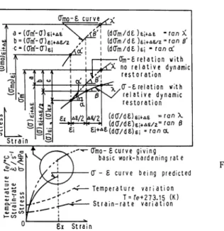
Figure 1 shows the schematic illustration representing the initial conditions of numerical calculation for predicting the <j— e curve by Runge-Kutta-Gill method in which equation (2) is employed. The lower illustration shows some curves giving the variables concerned in the calculation. amo— e curve is the basic temperature flow curve observed at the varying strain-rate to be considered in the calculation and at basic temperature. When the <jmo— e curve is known data, the value of {dom/de) in equation (2) can be

calculated by equation (5).

(don/d£)£,ejo={damo/d£)e,ijo (5)

The upper figure encircled by the solid line illustrates some variables on stress and strain concerned in the numerical calculationin strain increment Ae. (In the present caculation, ^£=0.004.) The strain, £x, and stress, (<j)ex are the initial values, et and (a)£i% respectively. Et+Ae and (<r)ei+A£ are the calculated

results (computer output), ex+Ae and ((j)£x+4£.

Basic stress, om", in the strain increment is the terminal stress attained at Et +Ae by deformation with basic work-hardening rate. Therefore, a* is the stress of om—e curve at strain, ei+Ae, and can be

NAKANISHI i EXACT PREDICTION OF THE FLOW CURVES AT ELEVATED TEMPERATURES 15 (Tmo-£ curve^^ <3 =((Jm'-(T)£i+Ae b=((Tm'-0')e;*A£/2 c =(crrrf-0")ei *

_7f

(dO"m/d£ )ti+At -tan X

(dCTm/d£)fci+A£/2siran 0' IdOm/dS )ei - tan al

-Ofn-£ relation with ynamic _I_L^X no relative dyn

! i'£[ restoration X/0"-£relation with relative dynamic restoration (d(T/d£)6ifA£ =ran\ (d(7/d£)ei+A€/2=^n $ £i+A£(d(T/d&)ei * tan ol

.*-"*" Omo- 6 curve giving

basic work-hardening rat e

0" - £ curve being predicted

Temperature variation T = fe+273.15 (K)

Strain-rate variation

Ex Strain

Fig. 1 Graphical expression of some variables con cerned in the numerical calculation for pre dicting the flow curve by using the work-hardening rate equation (Ae: Strain increment in Runge-Kutta-Gill method)

energy in the strain increment, AE and Ate, are calculated by equations (7) and (8) , respectively.

CTm' —(arno)ei+A£~ Wmotet + Mei W

AE = 0.5(a€i+<Tet+*€)Ae (7)

Ate = {0AE)/(JCp) (8)

where fi is constant, (J3 = 0 for isothermal deformation and £ = 1 for adiabatic deformation) , J the mechanical equivalent of heat (J = 4.2J/cal) , C and p specific heat and density of a material, respectively.

In the present work, the basic temperature work-hardeningrate equation, equation (9) , is introduced

so that the basic temperature flow curve at the varying strain-rate being considered can be determined by

numerical calculation.

(dOno/d£)e*joMda0/de)e*bjo+(7s/e)\((ro—Omo)\exp(qs<Tno2) (9)

where the first term in right hand side equation is the work-hardening rate observed at the basic

temperature To and at the basic strain-rate e6, (Eb should be fixed arbitrarily to some value such as Eb=\s~l.) , the second term the relative work-hardening rate (for which, 7S>0) or the relative dynamic recovery rate (for which, 7S<0) , and ys and qs are the experimental parameters. The numerical calculation for predicting the amo— e curve by using equation (9) is performed in the same way as that by using equation (2) and described previously. Values of the first term and Go are calculated by using equations (10) and (11) and the fixed flow curve, ab—e curve. (The flow curve, ab—e curve, should be determined beforehand by experiment at basic strain-rate, e'b, and at basic temperature, To.)

{dOo/dE )e,ib,To = (d(7b/d£ )£,k bjo (10)

(Jo —{ob)£i^A£ —{ob)£iJr(om(^£i (11)

3 . Development of the work-hardening rate equations with refering the experimental

flow curves of OFHC copper 3 . 1 Experimental data

16

«3e»;fc»X»«8f%«ft

£ 30 -^ (1988)

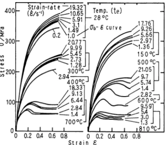
the experimental parameters involved in the work-hardening rate equations were prepared. The 7 mm diameter and 10 mm height test pieces are annealed OFHC copper of 99.995 wt% Cu specimens having grain diameter of 0.065mm. Compressive testings were performed by using cam-plastometer. The sub-press containing the testing specimen is heated by the electrical resistance furnace. Specimen's temperature is measured by using the 0.3 mm diameter alumel-chromel thermo-couple and digital pyrometer. The sub-press is taken out from the furnace at slightly higher temperature than the testing temperature and placed on the cam-plasto meter. Then testing is started at the testing temperature. Colloidal graphite (Oil-Dag) is used for lubrication between the tool and specimen interface and for prevention of oxidation of the specimen. Figure 2 shows the flow curves observed by the experiments. Both temperature, te (°C) , and strain-rate, e, are constants during deformation. The flow curves are

refered in the numerical analysis described below.

3 . 2 Procedure and computer program of the numerical analysis

Figure 3 shows some figures illustrating the procedure of the numerical analysis for determining the

parameters and terms involved in the work-hardening rate equations. Figure (A) represents the flow curves, q-e curve observed at T and £ and amo-e curve at To and £, which are refered from the experimental data shown in figure 2 and used in the analysis.

(1) Determination of the values of y0 and q

The values ofexperimental parameters, y0 and q, are determined by the numerical analysis using the

equations (12) and (13). Equation (12) is work-hardening rate equation in which both (da/d£)D=0 and

the intermediate experimental parameter, 7, given by equation (13) are substituted into equation (2).

Then, equation (12) contains only one experimental parameter.

The m numbers of data pairs, et and at (and (da/dE)£i written as Di) , are quoted from the

experimental data and used in the present analysis. If the flow curve, g—e curve, represents

work-softening phenomenon due to dynamic recrystallization, the above data pairs are prepared from the

flow curve between the strain, £=0, and the strain at peak stress.

(da/d£)£,£J=(dam/ dE)£,£JO—(y/e)(am —o)

(12)

7=7oexp(tf<72)

(13)

Figures (B) ~ (D) show the procedure of the analysis. The solid lines and points plotted with open

circles in (B) represent {da/dE)-£ curves calculated by numerical calculation using the equations

(5), (6) and (12) with considering the initial conditions of numerical calculation described in article 2.

The curves are the results obtained by numerical calculation in which some different values of y,(ya,

lb, ••*, Jg), are substituted into equation (12).

Those 7-values are prepared by equation (14). Equation (14) is introduced so that nearly

equi-difference of (da/dE) value between adjacent (da/dE)-e curve is achieved at individual strain, £tt

(plotted by the open circles).

Then, all data is most available to interpolation procedure for determining the value of 7, (yt at strain

£*), bywhich thesame value of(da/dE) as thatofexperiment can beobtained bythenumerical calculation.

7= Ue)logio(M), M= l, 2,

, 7

(14)

where A is the constant and can be fixed arbitrarily. (4 = 300 in the present analysis)

Figure (C) shows the procedure for determining the value of 7.

The open circles and solid line represents the {da/dE)-y relation prepared from the results shown in

figure (B). Referingto the experimental value of work-hardening rate, Di, and (da/dE)— 7 relation at eu

NAKANISHI : EXACT PREDICTION OF THE FLOW CURVES AT ELEVATED TEMPERATURES 17

data pairs, ((dcr/de), 7), prepared. In the illustrated case, 2nd order polynomial interpolation is adopted

to the data zone II in which the value of Di is contained. Combining at given from the experimental flow

curve at eu the data pairs, ( 7- , at), is obtained. The above procedure is performed at all individual

strain, Et, j = l to m, and m numbers of data pairs are obtained.

If the value of Di is not contained in the (da/dE)— 7 relation prepared by foregoing numerical

calculation, yt is determined by extrapolation or larger value of A in equation (14) should be used in the

analysis. Figure (D) shows the linear In 7 and a2 relation obtained by plotting the data pairs, ( yt , a2). Optimum values of y0 and q are determined so that the a— e curve calculated by numerical calculation

GS)

Strain-rate ~>19.32" it/*'1) ^-10.65 -5.91 0 0.2 0.4 0.6 0.8 0 0.2 0.4 0.6 0.8 Strain £

Fig. 2 Experimental flow curves of annealed OFHC copper at some constant strain-rates and at

some constant temperatures

(A) 0~mn-S curve

^-constp^f^T

(E) Determination

of 10(7/98)01 c- c. c 61 £1 £m \ Calculated with the

V determined values of £and <7

\

*}Experimental data

" 36/dI

In &

±tq£

(B) o Computed data (O Determination of A • Experimental data Using 2 nd order poly nomial

interpolation adopted at an appropriat e zone,I or II or 11, £i = const. m r-(fl.Oi) ^

(D) Deter mination of /o and Q

lnr-=lnfc+c((jz

Fig. 3 Figures explaining the sequences of the analytic procedure for determining the parameters, yQ and q,

18

«gft*»X»«ffi%«£

%30 -^ (1988)

in which the equations representing the amo— e relation, equations (5), (6) and (12) and equation (13)

substituted the values of y0 and q are employed is best fit to the a —E curve observed by experiment. (2) Determination of |(3a/3e)D| term

After completion of the determination procedure of the values of yQ and q, the values of | (da/dE)D | are determined by the numerical analysis.

The experimental values of (dcr/de), (expressed with the open circle points in figure (A)) , given from the a—E curve representing the work-softening phenomenon are refered in the analysis. Difference between the experimental value of (da/dE) and that calculated with considering only dynamic recovery in which both values of y0 and q are already determined gives the approximate value of |0<j/8e)D| at an

individual strain as shown in figure (E).

The above differences are used to determine the |(3<j/3£)d| term. The details of the analysis is

described in 3 • 3 (3).

(3) Computer program for determining the experimental parameters

Figure 4 shows the interactive computer analysis program which is constructed in accordance with the

analysis procedure described in 3.2. (l) and (2). The procedure of correction and optimization of the determined values is also attached to the program. For determination of the experimental parameters, ys

and qSj in equation (9) , the same computer program, in which the equations (9) , (10), (11) are used instead of the equations (2), (5) , (6) and the procedurefor determining the |(3a/3e)D| term is omitted, is prepared.

Variable parameter, y j y= ysexp(qsano2) I, in the program is positive value for £> £6, while negative

for £<£b. (7=0 at £=£b)m 3 . 3 Results of analysis

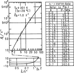
To= 301 K(28'C) and Eb—l s"1 are set as the basic temperature and basic strain-rate respectively, and the analysis using the computer program shown in figure 4 is performed.

(1) ab— e curve, and computer program for predicting the amo—e curve

The values of ys and qs in equation (9) are determined by refering the a —e curves observed at te =

28°C in figure 2. The results reveals that the value of ysis dependent of £ and qs=0. Then, equation (9) is simplified as equation (15). Figure 5 presents the data representing the ab and e relation, (a—E curve observed at te = 2&V, and £=l s~x in figure 2), and the relation between ysand £ obtained by the present analysis. (ys at e<1.49 are shown by the normal scale.) The ab—e curve is used in the numerical

calculation by expressing the segmental 2nd order polynomial equations. The ab—e curve at £>0.7 is

given by a6=384.6£0165. Equations (16) give the mathematical representation of 7sthat are installed in the computer program for predicting the amo— e curve.

(damo/'dE)£;£jo=(da0/'de)£;£bj0-\-(ys/'£)\(a0'' —amo)\ (15)

£^1.49 7*=exp| -0.0995(ln£)2+2.0553(ln£')-r-1.4988 I 0.7^£<1.49 75=19.277(ln£")2+17.389(ln£')

0.2^£<0.7 75=-0.278(ln£)2+0.452(ln£')-3.553

£<0.2 7*=-5.0 (16)

The computer program for predicting the amo— e curve is constructed with the equation representing

the ab— e relation and the equations (10), (11), (15) and (16). Input data of the program is the strain-rate

variation in deformation process. The program is installed in the analysis program shown in figure 4 and also the flow curve prediction program described later as the subroutine program. The program can also be used for predicting the amo—e curve of the material having different initial grain diameter when two

NAKANISHI : EXACT PREDICTION OF THE FLOW CURVES AT ELEVATED TEMPERATURES 19

procedures described below are added, (i) The procedure for determining the values of ab at some strains

as shown in figure 5for the material having specific grain diameter by applying the Hall-Petch relations,12

and (ii) the procedure to construct the segmental 2nd order polynomial equations for e^O.7 and power

equations for £>0.7 representing Gb and £ relation.

(2) 7o and q

Figure 6 shows the values of y0 and q with regard to the values of te (or T) and £. Figure (A)

presents the relations between In yQ and In £. The relations can be expressed by equation (17).

7o=ecaexp(C6)

(17)

where both Ca and Cb are the temperature dependants.

Figure (B) shows the relation between Ca and te, and the functional expression of the relation for

computer program is given by equation (18).

|INPUT DATA (FLOW CURVE AT T K AND £ s1 )

|EXPERIMENTAL WORK-HARDENING RATES AT STRAINS,^ |CALL SUBROUTINE (BASIC TEMPERATURE FLOW CURVE )|

CALCULATION OF WORK-HARDENING RATE AND r

RELATION AT EACH STRAIN OF STRAINS,fci, [NUMERICAL CALCULATION BY USING EQS.(5),(6) AND (12) WITH SOME VALUES OFp )

DETERMINATION OFf GIVING EXPERIMENTAL WORK-HARDENING RATE AT EACH STRAIN OF STRAINS,£|, fUSING 2ND ORDER POLYNOMIAL INTERPOLATION ]

m

inf AND 0"2 PLOT OF THE DATA PAIRS OF f AND

EXPERIMENTAL STRESS ,0~ ,AT STRAINS,t\, |

3

DETERMINATION OF £ AND q IN equation, In f-= In Jo + 90^

U

~T

/ CALCULATED FLOW CURVE COINCIDES NO./wiTH EXPERIMENTAL ONE (NUMERICAL

CALCULATION BY USING EQS. (5),(6),(12) AND (13) WITH THE VAT.URS OF ft AND <7 '

^ES

NO. /PROCEED THE ANALYSIS OF THE DYNAMIC , RECRYSTALLIZATION TERM

" \YES,

SUBTRACTION OF EXPERIMENTAL WORK-HARDENING RATE

FROM CALCULATED ONE AT EACH STRAIN OF STRAINS *

1

FUNCTIONAL EXPRESSION OF THE DYNAMIC RECRYSTAL-LIZATION TERM [DETERMINATION OF THE PARAMETERS,

Ha, HbAND£o IN EQ. (21) J^

~T

/CALCULATED FLOW CURVE COINCIDES WITH

/EXPERIMENTAL ONE \NO

[NUMERICAL CALCULATION BY USING EQS.(2), \(5),(6) AND (21) WITH THE VALUES OF

\ fr, q ,Ha ,Hb AND 6o 1 ^ v ^ .

/PROCEED THE ANALYSIS TO ANOTHER \YES

^DEFORMATION CONDITION ±np. (STOP^

IFUNCTIONAL EXPRESSION OF THE PARAMETERS, «, q Ha HbAND8o WITH REGARD TO BOTH TEMPERATURE AND STRAIN-RATE [OUTSIDE THE PRESENT PROGRAM ] 1

Fig. 4 Flow chart of the interactive computer pro gram used for determining the parameters, y0 and q, and term |Oa/3£)D| in the

work-hardening rate equation

10H 5X10? 10 -5X10: • "I....| i i11 n i n/ - To=?301 Ue =28 £b=i.o K °C)

s-1 /

/.

-

-/

-/I

MM I I I I I Mill 1 * ? f^ 1n ?n c n m

X10^

^ 50 10. 10 0 -10 LT. + r

m

0 5 0 7 1xc»2 £/s"1 a<

ob-£ curve data

Refer to Fig.2 £ fT/MPa 0 0 _9-8 0 0? 3$.2 0 04 7R.4 0 ₀₇ 179.4 o 1 1R1.7 0 1 3 1QR.n o _{1 fi} 777.5 0 18 71b.? 0 ?n 74A.9 n ?3 7fifi.fi 0 ?r 787.7 n 3 797.9 o 34 309.7 0 37 3l9.fi 0 ₄ 375.4 n 45 334.7 n 5 343.0 o S5 349.9 0 fi 3R4.ft o•fifi 359.7 _JQ.•7 362-6

20 _{ft&K^X^&mftnS H30^ (1988)}

Figure (C) gives the relation between Cb and te that can beexpressed byequation (19) for computer

program.

te>600 (°C) Ca=0.95

te<600 (°C)

Ca = 387.05X10-nie3-594.6X10-8^2+272.76X10-5ie+0.618

(18)

C6 = 2.6436£e01036 (19)

The parameter, q, is dependent to T but notto £, and given by equation (20) as shown in figure (D).

q= 0.0104exp( - 5340.7/T) (20)

(3) |Oa/3£)D| term

Figure 7 presents the examples explaining theanalysis for determining the values of | (da/d£)D | term.

1.1 1.0 0.9 0.8 1 300°C-| 150°C '-In %>= Cain8+ Cb J I L 2 In a/s-1

-(B)*-^

» — i 1 r _Z_. i i i _.l I I i 100 500 800 te/°C 6 7 In te/°C

Fig. 6 Both strain-rate, £, and temperature, te, dependence of the parameter, /0, and temper ature , T, dependence of the parameter, q

1000

° Experimental data

Calculated with considering the dynamic recovery term — Calculated with considering both the dynamic recovery and

recrystallization terms 1000rr fe=700*C 6 =9.13 s"1 150r (B) fe=700 °C 6=18.33 s'1 150r (B)

S^Vo^'oVe

°I

0.5 6 &=2900/s <7 =4.301x10"5MPa"2 #a=88 2 HPa/s ///>= 87.39 i- eo=0.475 #=1496/s s <7 =4.301 X10"5 MPaz 2 //a=686MPa/s •200 100 (O I Ha= 68 6 MPa/s —^ '""i jl •>* .60= 0.41 <^ 60 0.5 6 _—cdU 0r 1 1 i^ni^_{0 g \5}0.5 £

NAKANISHI ! EXACT PREDICTION OF THE FLOW CURVES AT ELEVATED TEMPERATURES 21

The broken lines in figures (A) and (B) are the (da/dE)- e curve and a —£ curve calculated numerically

by using equation (2) in which previously determined values of y0 and q and | Oa/3e)D| =0 are

substituted. While, the open circles plotted in the same figure represent the experimental data.

The differences between the values of (da/dE) observed by experiment and those calculated

correspond to the values of |(3j/8e)D| at individual strains.

Refering to the above differences, the values of | (da/3e)D I term at strains of the open circle points are

determined and functional expression of the term is investigated. The results of the analysis performed by

refering the a~E curves at £e^500 (°C) in figure 2 reveals that the term |Oa/3e)D| canbeexpressed by

equation (21). The values ofexperimental parameters, Ha, Hb and £0 involved in equation (21) are also

determined in the present analysis.

|Oa/a£)DH(r/a/£)exp|-r/6(£-£o)2l

(21)

The values of Ha, Hb and e0 could be determined directly by refering the equation to the relations

between the above difference of work-hardening rate and strain. It is yet required some correction of the

values of the parameters (especially of Ha) determined by the above procedure, because the rate of

dynamic recrystallization is affected with the work-softening (stress reduction) due to dynamic

recrystallization. The computer program shown in figure 4 involves the confirmation and correction

procedure in which theflow curve is calculated by using theequations (2) and (21) and compared with the

experimental values. Then, optimum values of the parameters, Ha, Hb, and e0 are determined by means of 2 to 3 times trial and error method. The solid lines in figure 7, (A) and (B) represent the results of numerical calculation using the values, Ha, Hb and £o, written in the figures. Excellent agreements between the calculated a~E curves and those observed by experiment can be confirmed. Figure (C) shows the values of |(3cr/3e)D| in the present calculation.

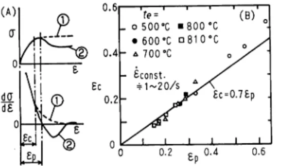
(4) Critical strain hardening energy, Ec

Figure 8 shows the results of analysis concerning the relation between the strain at which dynamic

recrystallization occurs and the strain at peak stress. In the present analysis, the strain at which

difference is found between the (da/de)-e curve calculated with considering only dynamic recovery and that with considering both dynamic recovery and dynamic recrystallization is £c as illustrated in figure

(A) , and figure (B) shows the results of the analysis. The results are obtained from the above analysis

refering to all flow curves observed at temperatures above 500°C in figure 2. It could be found that the

1 1 1 1 te = _ o 500°C "800 T 1 1

•c

(B)°

• 600°C °81 0°C o y - a 700 °C 0 yS - Sconst. = 1~20/s V £c=0.76p . / i i i 1, 1

JL-0.2

£p0.4

0.6

Fig. 8 Strain ec, at which restoration due to dynamic recrystallization starts, versus strain ep at peak stress

® : Calculated with considering dynamic recovery

22 _{3 e f t * » I » « 8 f % Wi & H 30 ^ (1988)}

equation, ec=0.7£p , exists between £c and ep. Deformation energy required for deformation from £=0 to £c can be considered as the critical value of the energy required for occuring the dynamic

recrystallization.9)10) Figure 9shows the relations between Ec and In £. The relations can be expressed by

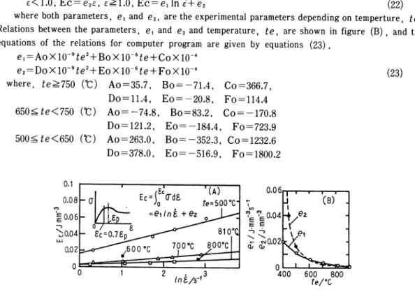
equation (22).

£<1.0, Ec=e2£, £^1.0, Ec=e1lri£+e2

(22)

where both parameters, ex and e2, are the experimental parameters depending on temperture, te.

Relations between the parameters, e, and e2 and temperature, te, are shown in figure (B), and the

equations of the relations for computer program are given by equations (23).

e^AoXlO-^e'+BoXlO^e + CoXlO-4

e2 = DoX10-9£e2+EoX10-6£e + FoX10-4

(23)

where, te^750 (°C)

Ao=35.7,

Bo=-71.4,

Co=366.7,

Do = 11.4, Eo=-20.8, Fo = 114.4 Ao=-74.8, Bo=83.2, Co = -170.8 Do = 121.2, Eo=-184.4, Fo = 723.9 650^£e<750 CC) 500^£e<650 (°C) Ao = 263.0, Bo=-352.3, Co = 1232.6 Do=378.0, Eo=-516.9, Fo = 1800.2 600 800 fe/°C

Fig. 9 Both strain-rate, £, and temperature, te, dependence of the critical energy, Ec, required for occur

ing dynamic recrystallization

100 50 Ha =9.Qexp{lnHao+THa) 1n (MPa/s-1) 10 5 80^ ^ Hb- 85046.5, 0.8 1.0 1.2 1.4 (//r)/io"3K_1 (A) z te-o 500°C • 600°C a 700 °C -2.0 200 400 600 800 fe/"C i i 0.02 0.04 0.06 0.08 0 200 400 600 800 Ec/J mm' fe/*C

Fig. 10 Both strain-rate, £, and temperature, te, dependences of the parameters, Ha, Hb and £o (Ec: Re

NAKANISHI ! EXACT PREDICTION OF THE FLOW CURVES AT ELEVATED TEMPERATURES 23

te<500 (°C) Ao = 300.2, Bo = -342.4, Co = 1090.3

Do = 7130.5, Eo =-7236.9, Fo = 18518.9

(5) The equations giving the values of Ha, Hb and e0

Figure 10 shows the results of analysis for constructing the equations expressing the relations between

the parameters Ha, Hb and e0 and the deformation conditions £, te (or T) and Ec. It could be found that

In Ha and ln£ relations at some constant temperatures represent parallel curves. Then, the relation between Ha and both te and £ can be expressed by equation (24).

r/a=9.8exp(ln Hao+Tha) (24)

wherethe parameter, Hao, is the dependent to £ and parameter, Tha, to te. Figure (A) represents the relation between Hao and £ and (B) the relation between THa and te. Those relations are expressed by the equations (25) and (26).

//ao = exp|A2X10-4(ln£)4+B2X10-3(ln£)3+C2X10-3(ln£r+D2X10-2(ln£)+E2|

(25)

where £^1.0 A2= -26.545, B2=31.392, C2= -260.687, D2=120.442, E2 = 2.8266 £<1.0 A2=370.936, B2= 308.646, C2=936.838, D2= 133.07, E2 = 2.8235 r//a=A3X10-6^2-r-B3X10-3^-f-C3 (26)

where £e^600 (°C) A3=-6.152, B3=5.707, C3=-1.17 400^ie<600 (°C) A3=-16.87, B3= 18.77, C3=-5.15

te<m (°C) A3=-7.0, B3= 11.4, C3=-3.78

The parameter, Hb, is dependent toT and can be expressed by equation (27) as shown infigure (C).

#6 = 85046.5/T (27)

Figure (D) shows the relations between e0 and Ec at some temperatures. Those relations can be

expressed by equation (28).

e0=SiEc + S,

(28)

where both Si and S2 are the temperaturedependents as shownin figure (E) , and can be expressed by

equation (29).

te^SOO (°C) S1= 251.02X10-6£e2-246.42XKT3£e+68.8

ie<500 (°C) S, = 15.43X10-6£e2 + 8.98X10-3£e

S2=-44.66X10_5£e + 0.4831 (29)

(6) Repetition of dynamic recrystallization process

Figure 11 shows the schematic illustrations explaining repetition of dynamic recrystallization process and an example of the analysis of the phenomenon. Figures (A-l) ~ (A-3) are the illustrations showing

the a—£ curve, variation of strain hardening energy, E, and variation of work-softening, |(8a/8£)D| , in

the deformation. Those figures explain that dynamic recrystallization occurs repeatedly whenever work-hardening energy reaches the value of critical energy, Ec. The results of analysis reveals that work-softening rate due to dynamic recrystallization appeared in n'th order can be estimated by equation (30). Equation (30) is given from eq. (21) by multiplying the correction facter l/4n_1. Strain e0 in

equation (30) is measured from the strain at which the strain-hardening starts. (Refer to figure 11.)

|Oa/a£)DHI(//a/4n-1)/£|exp|-//6(£-£0)2|

(30)

Figures (B) ~ (D) show the results of analysis with referingto the o— e curve observedat £e= 700 °C and £= 1.4s_1. Figures (B) and (C) show comparisons of the (da/dE)—e curve and a—e curve obtained by numerical calculation with those observed by experiment respectively. The broken lines are the calculated results in which \(da/d£)D\ = 0 is substituted in equation (2) , the single dotted lines in which

24 _{t t j e » * ¥ X ¥ S B F} recrystallization £ r (p)

, ,jW ;n=2

^10°l-IS 30 -^ (1988) fe=700°C £=1.4/s ° 5 Experimental data [—~ —} Predicted by numerica calculation ojuj 0>|CI> Q J_L *«2 5 2/s c , q=4.301x10"^MPa" //a-181.3 MPa/s 221 Hb=S7.39 0.5 6 ^=0.26

Fig. 11 Interpretation of repetition of dynamic recrystallization

(D :Calculated with considering dynamic recovery, © :Calculated with considering both dynamic re covery and single dynamic recrystallization, (3): Calculated with considering both dynamic recovery and repeated dynamic recrystallization

( start )

INPUT DATA

o:STRAIN-RATEVARIATION DATA o:TEMPERATUREVARIATION DATA

OR INITIAL TEMPERATURE, feo o:FINAL STRAIN, £f I -£ RELATION OR £ -e- £RELATION OR £e-t RELATION* t RELATION* | B=0,Omo=((Jb) at 8=0 \

1 £i=£ .( Pinole/ = QmA

I .

CALCULATION OF CTmo AT STRAIN, £i+*£ BY RUNGE-KUTTA-GILL METHOD USING

EQS.(10),(11),(15) AND (16) AND

Ob - 8 CURVE * £ - £ + * £ |no. ffrno - 8 CURVE* i =0 , 0=(Cfoio)at £=0 ,J=1,I=0 ,^JS=0 ,£s=Q ,0U)-0,E«0, te=teo |~Si =£,( (T)ei =CT ,J=j+l| CALCULATION OF (J, AE AND A f e AT STRAIN, £i+A£,BY RUNGE-KUTTA-GILL

METHOD USING EQS,(2),(5) ~ (8) AND (17) ~ (20) , 0"mo - 6 CURVE* AND SUBROUTINE PROGRAM, SUBDRC £=£+*£. (T(J)=0.te=te+&te.E=E+*E J)

w

&

j YES. < 0(1)>CT(2)<(J(3)AND 8>8s +£cQ , \ YES, I E=0 , s=l , £s= £-*£ 1 CT(l)<-fJ(2) , Ol2)<-Q(3) , J=2 V NO.

®-DISPLAYAND PRINT THE RESULTS

( (7-8CURVE AND fe -8CURVE )

( STOP ) CALCULATION OF Ec BY USING EOS.(22) AND (23) NO. < E^Ec> ,9S/D~ ( RETURN

El^ED

CALCULATION OF|(8C78£)ol BY USING

EQS. (24) ~ ( 30)

( RETURN )

Fig. 12 Flow chart of the computer program for predicting the flow curves t: Time (s) , Ae = 0.004, I, J and S: Control parameters of the program *= Expressed by a series of sectional 2nd order polynomial equations

NAKANISHI : EXACT PREDICTION OF THE FLOW CURVES AT ELEVATED TEMPERATURES 25

equation (21) is substituted in equation (2) , and the solid lines in which equation (30) is substituted in

equation (2). Figure (D) presents the variation of |Oo73£)D| calculated by equation (30). 4. Computer program for predicting the a~e curves

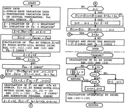
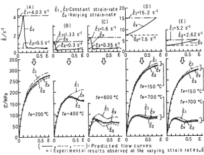
Figure 12 presents the flow chart of computer program for predicting the a— e curves. Input data for computation are strain-rate variation, temperature variation or initial temperature and final strain. Output data are a— £ curve and temperature variation in the deformation. Figure 13 shows the examples of g— e curve predicted by using the computer program, figure 12. Input data are deformation temperature written in the figures and strain rate variation, £„, shown in the upper figures and observed by upsetting

by oil-hydraulic press, (figures (A) - (C)| , and by constant compressive ram speed by cam-plastometer,

(figures (D) and (E)| . The solid lines in the lower figures show the a—e curves predicted and the open circle points plotted in the same figures represent the stresses at some strains observed by experiments performed under the same deformation conditions used for the computations. Excellent agreements are confirmed between the a —E curves predicted and those observed by experiments. Furthermore, some calculation to estimate quantitative effect of the varying strain-rate on a —£ curve are performed. The single dotted lines and broken lines are the a—E curves predicted with considering the constant high

strain-rates, £u or constant low strain-rates, £2, which are involved in the individual varying

strain-rates, £v.

The a—E curves under the adiabatic deformation conditions are also predicted with considering both varying strain rates and varying temperatures. |C = 0.093 (cal/g°C) and ,0 = 8.96 (g/cm3) are substituted

in equation (8)|

i ... .( £i , cr-Constant strain-rate 20r

rti=±v?±_ £v:Varying strain-rate A

(o 15r-. (E)

£l=5.2 s"1

I 52=2.62 s"1

0.5 £ 0 0.5 £ 0 0.5 £ 0 0.5 £ 0

( , , )=Predicted tlow curves

o : Experimental results observed at the varying strain rates,£v

Fig. 13 Examples of the flow curves predicted at three rate conditions, i. e., at two constant strain-rates, e, and e2, and at one varying strain-rate, £v, in the individual case, (A) —(E) , by using the computer program shown in Fig. 12 The points plotted by open circles are the experimental data obtained at the varying strain-rate, £v, in the individual case, (A) —(E).

26 _{j e * * ¥ x * « « f f t « f t iMo-t 0988)}

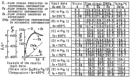
Table 1 shows the mutual comparisons of the stresses predicted under the isothermal deformation condition or the adiabatic deformation condition or measured by experiment at three strain values. The strain rate conditions are the same varying strain-rates, £Vt as shown in figure 13.

The a—E curves under the adiabatic condition show slightly low stress level compared to those under

the isothermal condition. Much remarkable difference between the flow curves under the isothermal

condition and those under the adiabatic condition could be predicted in large deformation. (Refer to

appendix 2)

Table 1 Comparison of the flow curves measured or predicted by showing the flow stresses at three strains 0"i :FLOW STRESS PREDICTED IN

ISOTHERMAL DEFORMATION

0"a :FLOW STRESS PREDICTED IN

ADIABATIC DEFORMATION

0~e :FLOW STRESS OBSERVED BY

EXPERIMENT

(fe)a :DEFORMATION TEMPERATURE

INADIABATIC DEFORMATION ^ 2

K

200r—(r\ o(7e 440-420 400 0 0.5 £

Example of the results Input data

/Strain rate: £v,(B)in Rg.13\

\Temperature: fe=400*c / Input data fcv and te (A) in Fig. 13 fe=200°C (B) in Fig. 13 fe=400°C (C) in Fig. 13 fe=600°C (D) in Fig. 13 fe=150'C (E) in Fig. 13 te =150'C (D) in Fig. 13 fe«700°C (E) in Fig. 13 fe«700°C Strain _£__ ~0T5T JLJ_ 0.5 0.68 0.3 0.5 "OS" i i . 768

3d

_oTW JL_3_ JL5_ 0-58 JL1_

-Mb

Flow stress O/MPa

£\ ja_ JJL_ 226.8 260.0 27T5 169-9 175.2 157.4 _6M _&5J 641 26Q-6 3QQ-4 317.2 247.2 7^0" Too? _22± _BZ1 83.2 74.7

a

226-8 258-8 271.8 168-7 1604 15M Jl2A _6_L1 59.8 25 9-4 MM 314.0 24 6.3 m i 2M2 91.8

m

73.9

m

218-Q 25&j 274^ 168-9 171-7 160.5 69.4 6275 62.7 2J& JU 245.0 MM 297.9 _ m _&2£ _SM i M 66.6 Temp/°Cre mo, Jtel 212-6IA1A 226^ 240.1 409-5 419.2 427.3 605.4 609.0 TTTT

M

jM± 193.7 706-1 711-0 715-1 705.4

m

5 . Conclusions

Some experimental analyses are performed with refering to the experimental flow curves of annealed OFHC copper. In the present analyses, the work-hardening rate equation that consists of the basic work-hardening rate term, the dynamic recovery rate term and the work softening term due to dynamic recrystallization and the basic work-hardening rate equation that gives the value of basic work-hardening rate term are constructed. It has been reported that the dynamic recrystallization process is strongly

affected with the material's structure such as initial grain diameter. The above conditions can be involved

in the experimental parameters in the present equations. Application of the method to the other materials requires determinationof the experimental parameters involved in the two work-hardening rate equations. This can be achieved easily by using the interactive computer program for determining the values of the

experimental parameters in the work-hardening rate equations.

References

1) Kato,K.: J.Materials (##), 30-330(1981) ,95.

2) Hartley,C.S.& Srinivasan,R.: Trans.ASME, J.Engng.Mater. & Technol., 105-7(1983) ,162.

3) Dadras,P.: ibid., 107-4(1985), 97.

4) Hojyo,A., Chyatani,A, Yonetani,S.: J.Materials Sci. (^W4^) , 22-2(1985) ,90.

5) Yada,H. & Senuma,T.: J.Japan Society for Technology of Plasticity (8H4£finD,

NAKANISHI : EXACT PREDICTION OF THE FLOW CURVES AT ELEVATED TEMPERATURES 27

6) Okamura,S., Nakamura,T. & Nakanishi,K.: ibid., 16-175(1975) ,636.

7) Nakanishi,K., Okamura,S. & Nakamura,T.: ibid., 18-203(1977) ,990.

8) Nakanishi,K., Okamura,S., Fukui,Y. & Nakamura,T.: ibid., 22-246(1981) ,669.

9) Maki,M. & Tamura,I.: J.Materials, 30-329(1981) ,107. 10) Sakai,T.: 101th JSTP.Simposium text, (1985) ,11

11) Nakamura,T. & Ueki,M.: ^S^123SW^E*^ 18-3(1977) ,243.

12) Armstrong,R.W.: Advances in Materials Research,4, (1970) ,101-119, John Willey & Sons, Inc.

New York

Appendix 1-Computer analysis

Some CRT. hard copys are presented here according to the order of analysis, so that the intermediate results as well as the whole procedure of the computer analysis for determining the experimental parameters involved in the work-hardening rate equations could be understood. In the construction procedure of the work-hardening rate equations for a metal or an alloy, the basic temperature and basic

strain rate should be fixed at first. It should be noted that the basic temperature is the lowest limit

temperature at which the work-hardening rate equations are adopted.

While, there is no special restriction in setting the value of the basic strain-rate. In the present case, room temperature is set as the basic temperature by expecting that the work-hardening rate equations are

applied in warm and hot deformation and unit strain-rate, 1 s"1, is set as the basic strain-rate. The

experimental parameters, ySl in the basic work-hardening rate equation should be determined with refering the experimental flow curves which are observed at some constant strain-rates under the basic temperature. Present analysis reveals that the value of qs in the basic temperature work-hardening rate equation is always 0. Then, determination of the value of ys can be performed simply by comparing the

experimental flow curve with the flow curves calculated by using equations (9), (10) , (11) and the values

of 7s given as input data. Figure 14 is the CRT. hard copy showing an example of the above procedure.

Some points representing the experimental flow stresses at some strains are plotted at first on the stress and strain coordinate system in CRT. display. Refering to those experimental data, some flow curves which are available to determine the proper value of ys are calculated and displayed on the CRT.

In the present case, four different flow curves shown by the solid lines are calculated by using four different values of ys; i.e., 7*=10, 100, 200 and 300. Then, proper value of ys, by which the best fit flow curve to experimental one can be calculated, is determined from the above data.

In the present strain-rate, c= 5.91/5, 7s=139/s is determined as the optimum value of ys by interpolation procedure applied to the calculated relations between flow stress and ys and the experimental

flow stresses at some strains. The above interactive computer analysis are performed with refering some

experimental flow curves that are measured at some strain-rates, and the equations representing the relationbetween the valueof ys and strain-rate, e, is obtained. Then the computer program for predicting

the basic flow curve can be constructed with equations (9) , (10) , (11) and equation giving the value of ys.

(such as equation (16))

Followed analysis is to determine the experimental parameters of y0 and q in the dynamic recovery term and Ha, Hb and £0 in the dynamic softening term in the work-hardening rate equation at elevated temperature by using the semi-automated interactive computer program presented in figure 4.

The procedure for determining the parameters Ha, Hb and £0 is omitted for the materials representing only dynamic recovery. The following figures show a series of intermediate and final results obtained in

28 _{« J B * ; * : ¥ I ¥ B f l F f t * f t 30 •§• (1988)}

the analysis for determining the experimental parameters with refering the experimental flow curve at £= 18.33s"1 and at 700 °C . Table 2 presents the computer out put showing the basic temperature flow curve at £= 18.33s"1 calculated by the subroutine program that is installed in the present analysis program.

Figure 15shows theCRT. hardcopy representing the(da/dE)-e curves, (A) , and the a-£ curves,

(B) , obtained by the numerical calculations using the equations (5), (6) and (12) with some different

values of y given by equation (14). The plotted points by open circles represent the experimental data.

The values of y at some stresses are determined automatically by the numerical analysis, descrived in

3.2.(1), using the computer.

Figure 16 shows the values of y at some stresses and CRT. hard copy showing In y and g2 plots. Then

the values of y0 and q are determined from the linear relation between In y and a2, In 7= ln y0+qa2.

The optimum values of y0 and q are determined by trial and error method so that the best fit flow curve which is obtained by numerical calculation using the equations (5), (6) , (12) and (13) to the experimental

one is achieved. Figure 17 presents the CRT. hard copy showing confirmation that the values of y0 and q

Table 2 Basic temperature flow curve, amo-e curve, calculated by using the computer program

ED •

6 =

TIME STRAIN STRAIN STRESS STRESS

•5.91 s"1 t a -RATE 5 Omo Ob h •Experimental "v

data

300

( s ) < - ) (1/s) (kg/mm2)(kg/mm2) o T 0.000 E 0.000 V 18.330 Yl 0.000 Y1B 0.000 0.001 0.020 18.330 4.315 4.000

^_^200

0.002 0.040 18,330 8.633 8.000 ^D 0.003 0.004 0.060 0.080 18.330 12.598 11.678

4^^\*10°

18.330 15.652 14.511 0.005 0.100 18.330 17.839 16.500

&r^

10

0.007 0.120 18.330 20.642 19.100 cr 0.008 0.140 18.330 22.870 21.167

kg-mm~2

&y 0.009 0.160 18.330 24.522 22.700

"

4=135s-'

0.010 0.180 18.330 26.027 24.100 0.011 0.200 18.330 27.429 25.400 2D __ w 0.012 0.220 18.330 28.747 26.622 determined 0.013 0.240 18.330 29.969 27.756 at 5=5.91 s"1 0.014 0.260 18.330 31.096 28.800 0.015 0.280 18.330 32.015 29.650 0.016 0.300 18.330 32.824 30.400 0.017 0.320 18.330 33.525 31.050 0.019 0.340 18.330 34.118 31.600 0.020 0.360 18.330 34.876 32.311 a

'

i

i i i i i 0.021_0.022 0.380 0.400 18.330 18.330 35.451 35.837 32.844 33.200 D

D'5

E(£)

0.023 0.420 18.330 36.225 33.560 0.024 0.440 18.330 36.614 33.920 0.025 0.460 18.330 37.002 34.280 0.026 0.480 18.330 37.390 34.640 0.027 0.500 18.330 37.777 35.000

7ig. 14 Example of analysis for determining the 0.028_0.029 0.520_0.540 18.330 18.330

38.105 38.398

35.304 35.576 values of 7s at some strain-rates 0.031 0.560 18.330 38.657 35.815

0.032 0.580 18.330 38.881 36.023 0.033 0.600 18.330 39.074 36.200 0.034 0.620 18.330 39.315 36.424 0.035 0.640 18.330 39.522 36.616 0.036 0.660 18.330 39.695 36.776 0.037 0.680 18.330 39.833 36.904 0.038 0.700 18.330 39.936 37.000

NAKANISHI : EXACT PREDICTION OF THE FLOW CURVES AT ELEVATED TEMPERATURES 29

are proper ones by comparing the calculated (da/dE)—e curve and a—E curve with experimental ones, respectively.

(The comparison is valied only in the strain range between 0 to 0.3 in which the restoration process is only dynamic recovery.) Figure 18 shows the CRT. hard copy that represents the further analysis for

:Experimentaldata,DY2

5930.39

o:Experimental data,Y2

Fig. 15 Computed intermediate data and experimental data for determining the values of y0 and q in the work--hardening rate equation Deformation temperature, te= 700*0 , Strain-rate, e = 18.33 s_1

a Omo (dOmo/d£) cr (d(J/d£) <Jl

r-( - ) (kg/mm ) (kg/mm ) (kg/mm ) (s-1)

E Yl DY1 Y2 DY2 Y2*Y2 G 0.060 12.598 175.480 5.845 61.111 34.160 3518 780 0.100 17.839 124.747 7.400 40.000 5 4 . 7 6 3 3560 470 0.140 22.870 97.015 8.645 22.222 74.729 3918 480 0.180 26.028 72.668 9.400 15.000 88.361 3996 170 0.220 28.746 63.499 9.811 9.445 96.250 4167 230 0.260 31.096 51.149 10.100 5.000 102.002 4330 610 0.300 32.825 37.744 10.300 2.500 106.090 4407 890 u u u u _{idltmi mi INI llll mi mi llll mi nn nn} nn Mil mi mi nn Mil III! nn lire

5DDD -E In t=lnto + qa2 -IDDD _—B 5DD -: IDD - -^ q n mn mi mi mi mi nn mi nnMil nn nn nn Mil nn mi nnnn nn nn11rr 5D IDD I5D 2DD

Fig. 16 In7 and a2 plots and determination of yQ and q in the work-hardening rate equation

30 _{l B * * * I * » B f * « # * 30 -S- (1988)} ^D 3D M E e 2D 3 dD"_dE ID - ID -2D Go= 2900 q= .004 U) (O (A) I o:Experimental t data :Calculated _l I I I L_ D.5 E ED 4D 2D (B) o:Experimental data —:Calculated «X>«uuu600000 J I I I I L D.E

Fig. 17 Confirmation of the values of y0 and q determined by the numerical analysis

Deformation temperature, te= 70013, Strain-rate, =18.33 s_1

(£) (<0 (&)

Go= 2900 q= .004 Ha= 90 Hb= 87.39 Eo= .475

ED (A)

2S)J.fr«tf*ie-6i'l

\

«Q

—:Calculated o:Experimental data +:Approximate values of

dynamic softening term

o:Experimental data

JL

• 7 I I l i i T D.5 0 Calculated with considering dynamic recovery © Calculated with considering both dynamic recovery

and recrystallization

Fig. 18 Analysis for determining the dynamic softening term due to dynamic recrystallization Deformation temperature, te= 700'C ,Strain-rate, c= 18.33 s_1

NAKANISHI : EXACT PREDICTION OF THE FLOW CURVES AT ELEVATED TEMPERATURES 31

determining the values of experimental parameters, Ha, Hb and £o in equation (21).

Theoptimum values of Ha, Hb and e0 are determined bytrial and error method sothat the bestfit flow

curve to the experimental one is calculated by using the equations (2) , (5) , (6) and (21). Figure (A)

shows the approximate values of dynamic softening term at some strains which are used as reference data for the present analysis and (da/dE)— e curve for confirmation of the values of experimental parameters.

Figure (B) shows mutual comparison between the experimental flow curve and the a— e curves calculated

with considering only dynamic recovery and with considering both dynamic recovery and dynamic

recrystallization. (The optimum values of parameters, y0, q, Ha, Hb and £0 are used inthe calculation.)

Figure 19 is the CRT. hard copy representing final confirmation that the values of experimental

parameters determined bythe present analysis are correct values by comparing the (da/dE)— e curve and

g-e curve calculated with the experimental ones, respectively. (The comparison is valied in whole strain

range, because both restoration processes; i.e., dynamic recovery and dynamic recrystallization aretaken

into account in the calculation.)

Appendix 2-Examples of flow curve prediction in large deformation

Figures 20 and 21 present the CRT. hard copys showing the flow curves predicted up to large

strain, £= 2.5, by using thecomputer program, (figure 12). Figure 20 is the results calculated at constant

strain-rates and at constant temperatures. While, figure 21 is the results calculated at two types of

varying strain-rates during deformation under the isothermal or adiabatic condition. The strain-rate

variation in figure (A) is assumed with expecting a forging and (B) is assumed with expecting a extrusion.

Temp.= 700 (d G0= 2900 q= . Ha= 90 Hb= 87 3D egC) Strain 004 .39Eo= .475

"I

_{1 :Calcul} l o :Experi -Rate= (A) ated mental 18 da .33 ta (1/sec ED ) (B) — :Calculated o :Experimental dat e E 2D _ \ ID g dE ID D - ID

- V

(Nl E E X b 0" 2D o

f

f l I I l l l -2D C I I 1 1 1 1 D [ ] D.5 E 8 ] D.5 E 8

Fig. 19 Final confirmation as well as confirmation of the values of Hn, Hb and e0 determined by the numerical

analysis

32 _{%gi±¥T.¥Um%.m£ £30-51- (1988)} EDD _{£ =5 S'1} EDD _{5 =20 s"1} fe ^ R.T. 4DD D/MPa

^^^-300°C

2DD

f

__. 500°C

f

— 700°C n l " ' ' ' 800°C i i i i t te 4 ^^R.T. 4DD

" / ^

D/MPa

/ ^-^_-300°C

2DD

lU^—-

500°C

L

700°C

K~ 800°C D i i i i i i E D 2.5 E C8) (6) 2.5 £ =0.5 s"1

Fig. 20 Some flow curves predicted by the computer program, (Refer to Fig. 12) Both deformation temper ature, te, and strain-rate, £, are constants in the deformation. (R. T.: Room temperature assumed

as basic temperature) (A) Mr' _1 l _ l I I 4DD D/MPa 2DD DEFORMATION CONDITION j- ISOTHERMAL <3- ADIABATIC te r300°C 'a-300~482°C K500°C la-500~619 °C ;^700°C __'U700~765°C <3-800~848°C -J—i I i I E(£) DEFORMATIONCONDITION i - ISOTHERMAL a - ADIABATIC te j-300°C a-300~474°C ./500°C 500~597°C

Fig. 21 Some flow curves predicted by the computer program, (Refer to Fig. 12),

Two types of varying strain-rates and isothermal or adiabatic deformation are assumed in the flow curve prediction.