Shimura curves as intersection of Humbert surfaces and defining equations of QM-curves of genus two

Shimura curves as intersection of Humbert surfaces

and defining equations of QM-curves of

genus

two

早大理工数学科 橋本 喜一朗 (Ki-ichiro HASHIMOTO)

早大理工数学科 村林 直樹 (Naoki MURABAYASHI)

1

Introduction

Let $A$ be asimple principally polarized abelian variety of dimension two over the complex

number field $C$, and let End$(A)$ be the algebra of endomorphisms of $A$. Then, as is well

known, the Q-algebra $End^{O}(A)$ $:=End(A)\otimes zQ$ belongs to either one of the following

types:

(i) a CM field ofdegree four,

(ii) an indefinite quaternion algebra,

(iii) a real quadratic field, or

(iv) the rational number field Q.

Let $A_{2,1}$ be the moduli space of the isomorphism classes of $A$ with principal polarization.

The moduli of $A$ in each case has dimension 0,1,2,3, respectively, whose components in the

first three cases are called (i) CM-points, (ii) Shimura curves, (iii) Humbert surfaces. On

the other hand, it is also well known that the Torelli mapgives a birational morphismfrom

$A_{2,1}$ to the moduli space $\mathcal{M}_{2}$ of curves ofgenus two.

In this paper, we are interested in constructing, in concrete way, an $al$gebraic family of

curves of genus two whose jacobian varieties belong to the case (ii) above. Namely we

wish to find out an equation of a fibre space, the base space of which is a Shimura curve

and fibres are curves of genus two whose jacobian have quaternion multiplications. Call

such curves simply “QM-curves”. We shall give defining equations of algebraic family of

QM-curves in the case where the endomorphism ring is, generically, a maximal order $\mathcal{O}$ of

the indefinite quaternion algebra over $Q$ which ramifies exactly at

{2,3}

or

{2,5}.

To the

best of our knowledge, not a single example of such curve has been known before. Here we

should point out that examples ofdefining equations ofShimura curves have been given by

Kurihara [15], Jordan-Livn\’e [11]. However, they are not moduli-theoretic, hence are not

helpful for our purpose.

[7], one can find general approach, as well as concrete solutions in

some

cases, to the

similar problem for the case (iii), i.e., to construct families of curves of genus two whose

jacobian varieties have real multiplication ofgiven discriminant. (cf. $[2],[16]$). Especially,

Humbert gives explicite form of “modular equations” for discriminant 5 and 8, in terms of

the coefficients ofthe curves $y^{2}=f(x)$. Our idea is simply to combine these twoequations

in a suitable way. Indeed, if one can arrange the coordinate system in such away that the

two real multiplications generate $\mathcal{O}$, then the fibre space we are looking for will be obtained

asa component oftheintersection ofthe two Humbert’s families. The determination of the

possible components are carried out by studying quaternion modular embeddings of the

upper half plane to the Siegel upper half plane of degree two. Although the calculations

needed to find out the components are quite complicated, they can be perfomed by using

computer symbolic manipulation.

The main results are given as theorems 2.1 in

\S 2.

As an application, we can give an

equation of a family ofsupersingular curves of genus two over the field $\overline{F}_{p}$ ofcharacteristic

$p=3,5$

.

The proofs will be given in the latter sections. In \S 3, we recall brieflysome results

of Humbert [7] which are needed for our constructions. In

\S 4,

we study, in some detail,

quaternion modular embeddings of the upper half plane to the Siegel upper half plane of

degree two, in the case of the maximal orders of the quaternion algebra with discriminant

6 and 10. A more general treatment is given by [5].

2

Statement of

main

results

Let $B$ be anindefinite division quaternion algebra over$Q$, andlet $\mathcal{O}$ be a maximal orderof

B. We denote by $D_{B}$ the product of primes at which $B$ ramifies, and call it the discriminant

ofB. Let $\alpha\alpha’$ be the canonical involution on $B$, and let$Tr(\alpha)$ $:=\alpha+\alpha’,$ $Nr(\alpha)$ $:=\alpha\alpha’$

be the reduced trace, reduced norm on $B$, respectively. Then $\mathcal{O}^{(1)}$

$:=\{\alpha\in \mathcal{O}|Nr(\alpha)=1\}$

is regarded as a Fuchsian group of $SL_{2}(R)$ and the compact Riemann surface $\mathcal{O}^{(1)}\backslash \mathfrak{H}$ is

identified with the C-valued points ofthe Shimura curve $S_{B}$ (cf. [19],[20]). $S_{B}(C)$ has the

following interpretation. Let $\rho$ be an element of

$\mathcal{O}$ such that $\rho^{2}=-D_{B},$

$\rho \mathcal{O}=\mathcal{O}\rho$. The

existence of such element can be shown byusingstrong approximationtheorem, orby direct

construction of$\mathcal{O}$ (cf. $[8],[5]$). Then the involution of $B$ defined by _{$\alpha-\alpha$}“ $:=\rho_{1}^{-1}\alpha’\rho_{1}$ is

positive, and it satisfies $O^{*}=O$

.

Then we have

$S_{B}(C)\underline{1:1}\{(A, i, \Theta)|(A, \Theta)$

: principally polarized abelian

$surface\}$ $i:\mathcal{O}=*\rangle End(A)$

Rosati involution w.r.$t\Theta_{1\mathcal{O}}=*$

Hence we have a ratinal map

$S_{B}arrow A_{2,1}(C)\cong Sp(4, Z)\backslash \mathfrak{H}_{2}$ $\approx$ $\mathcal{M}_{2}(C)$

Now the problem we are interested to solve is to describe the image of the Shimura curve

$S_{B}$ in $\mathcal{M}_{2}$. More precisely, we look for an equation of the following form:

where $f$ is separable ofdegree 5 or 6 in $X$, and $\overline{Q}(s, t)=\overline{Q}(S_{B})$ is the function field of $S_{B}$

over Q.

Here we shall give an answer to this problem in the two cases where $D_{B}=6,10$. Our

results are:

Theorem 2.1 (i) Case

_of

$D_{B}=6$.

$S_{6}$ : $Y^{2}=X(X^{4}-PX^{3}+QX^{2}-RX+1)$, with $g(s, t)$ $=$ $s^{2}+(7t^{4}-8t^{3}+18t^{2}-8t+7)=0$, $RP$ _$=$ $\ovalbox{\tt\small REJECT}\pm(3t^{2}-2t+3)\{(5t^{4}+4t^{3}-2t^{2}+4t+5)\pm(t^{2}+1)s\}8t(t^{2}+1)(t^{2}-t+1)$ $Q$ $=$ $\ovalbox{\tt\small REJECT}(t^{4}+1)(2t^{8}-6_{2}t^{7}+3t-6t-2t_{2}-6t+2t(t-1)^{6_{2}}(t^{2}+^{5}1)^{2}(t^{4}-t+^{3}1)^{3t^{2}-6t+2)}$ (ii) Case

_of

$D_{B}=10$

.

$S_{10}$ : $Y^{2}=X(P^{2}X^{4}+P^{2}(1+R)X^{3}+PQX^{2}+P(1-R)X+1)$, with $g(s, t)$ $=$ $s^{2}-(t^{2}.-2)(2t^{2}+1)=0$, $P$ $=$ $\frac{4(2t^{2}+1)(t^{4}-t^{2}-1)}{(t^{2}-1)^{2}}$ $R=$ $\frac{(t^{2}-1)s}{t(t^{2}+1)(2t^{2}+1)}$ $Q$ $=$ $\frac{(t^{4}+1)(t^{8}+8t^{6}-10t^{4}-8t^{2}+1)}{t^{2}(t^{2}-1)^{2}(t^{2}+1)^{2}}$

Remark 2.2 The genera

_of

Shimura curves $S_{B}$ are zero

for

$D_{B}=6,10$

.

So

one

could

obtain the

_families

_of

QM-curves over $P^{1}$, while our

familes

are over the elliptic curve

$g(s,t)=0$. Indded, our

_families

are reduced to those over $P_{f}^{1}$ since the two

fibres

on

$(s, \pm t)$ are easily seen to be isomorphic.

By specializing $(s, t)$ to those points $(s_{0},t_{0})\in\overline{Q}^{2}$ such that _{$g(s_{0}, t_{0})=0$}, one canobtain as

many QM-curves defined over $\overline{Q}$ as one wishes. However, one should note that the curve

$Y^{2}=f(X;s_{0},t_{0})$ may be a split curve, i.e., the jacobian can split to a product of two

elliptic curves with complex multiplication.

Finally, we note that the reduction of a Shimura curve at the prime where $B$ ramifies

gives a moduli of supersingular abelian varieties (cf. [18]). Moreover, it is known that the

number of irreducible components of the moduli of such curves is one for $p\leq 11$ (cf. [12]).

Corollary 2.3 For $p=3,5$, a family

_of

supersingular curves

_of

genus two over the

_field

$\overline{F}_{p}$

of

characteristic

$p$ is given by the following equation:

(i) For$p=3$ $\overline{S}_{6}$ : $Y^{2}=X(X^{4}-PX^{3}+QX^{2}-RX+1)$, with $P$ $=$ $\pm 1-\sqrt{-1}$ $R$ $Q$ $=$ $\frac{(t^{4}+1)^{3}}{t^{2}(t^{2}-1)^{2}(t^{2}+1)^{2}}$ (ii) For $p=5$ $\overline{S}_{10}$ : $Y^{2}=X(P^{2}X^{4}+P^{2}(1+R)X^{3}+PQX^{2}+P(1-R)X+1)$, with $P$ $=$ $\frac{-(2t^{2}+1)(t^{4}-t^{2}-1)}{(t^{2}-1)^{2}}$ $R=$ $\frac{(t^{2}-1)}{\sqrt{2}t(t^{2}+1)}$ $Q$ $=$ $\frac{(t^{4}+1)(t^{8}-2t^{6}+2t^{2}+1)}{t^{2}(t^{2}-1)^{2}(t^{2}+1)^{2}}$.

3

A

work of Humbert

Let

$\tau=(\begin{array}{ll}\tau_{1} \tau_{2}\tau_{2} \tau_{3}\end{array})$

be a element of the Siegel upper halfspace $\mathfrak{H}_{2}$ of degree 2. Put $A_{\tau}=C^{2}/L_{\tau}$ with $L_{\tau}$ the

lattice generated by the columns of the matrix $(\tau 1_{2})$. Put $a=(11t_{2}^{2})$ and $b=(\begin{array}{l}11/2\end{array})$ .

For $z=(\begin{array}{l}z_{1}z_{2}\end{array})$ in $C^{2},\cdot$the 2-dimensional holomorphic theta function with characteristic

$\{\begin{array}{l}ab\end{array}\}$ is defined by

$\theta(z)=\sum_{n\in Z^{2}}e^{\pi i^{t}(n+a)\tau(n+a)+2\pi i^{2}(n+a)(z+b)}$,

where $n$ is written

as

a column vector and ${}^{t}v$ denotes the transpose of a column vector

$v$.

The following lemma is well known:

Lemma 3.1 Let$p,$ $q$ be column vectors in $Z^{2}$. Then

$\theta(z+\tau p+q)=e^{-\pi i^{t}p\tau p-2\pi i^{t}p(z+b)+2\pi i^{t}aq}\theta(z)$.

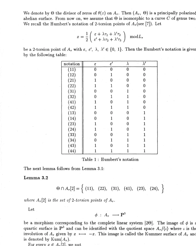
We denote by $\Theta$ the divisor of zeros of $\theta(z)$ on$A_{\tau}$. Then $(A_{\tau}, \Theta)$ is aprincipally polarized

abelian surface. From now on, we assume that $\Theta$ is isomorphic to a curve _$C$ ofgenus two.

We recall the Humbert’s notation of 2-torsion points of$A_{\tau}$(see [7]). Let

$x= \frac{1}{2}(\begin{array}{l}\epsilon+\lambda\tau_{1}+\lambda’\tau_{2}\epsilon’+\lambda\tau_{2}+\lambda’\tau_{3}\end{array})$ $mod L_{\tau}$

be a2-torsion point of$A_{\tau}$ with $\epsilon,$ $\epsilon’,$ $\lambda,$ $\lambda’\in\{0,1\}$. Then the Humbert’s notation is given

by the following table:

Table 1 : Humbert’s notation The next lemma follows from Lemma 3.1:

Lemma 3.2

$\Theta\cap A_{\tau}[2]=\{(11)$, (22), (31), (41), (23), (24), $\}$

where $A_{\tau}[2]$ is the set

of

2-torsion points

of

$A_{\tau}$.

Let

$\phi$ : $A_{\tau}arrow P^{3}$

be a morphism corresponding to the complete linear system $|2\Theta|$

.

The image of $\phi$ is a

quartic surface in $P^{3}$ and can be identified with the quotient space

$A_{\tau}/\{\iota\rangle$ where $\iota$ is the

involution of$A_{\tau}$ given by

$x-x$

. This image is called the Kummer surface of$A_{\tau}$ and

is denoted by $Kum(A_{\tau})$.

For every $x\in A_{\tau}[2]$, we put

and

$\overline{\Theta_{x}}$

$:=\phi(T_{x}(\Theta))$

where $T_{x}$ denotes the traslation by $x$

.

Since $2T_{x}(\Theta)\in|2\Theta|$, there exists aunique hyperplane $H_{x}$in$P^{3}$ such that theintersection

divisor of$H_{x}$ and $Kum(A_{\tau})$ is equal to the divisor $2\overline{\Theta_{x}}$.

$H_{x}$ is called the singular plane of $Kum(A_{\tau})$. From $now$ on, we denote $\phi((ij))(1\leq i,j\leq 4)$ by the same notation $(ij)$ and

call themdouble points of$Kum(A_{r})$. Then singular planes can be uniquely represented by

sixteen symbols $kl(1\leq k, l\leq 4)$ such that the following conditions are satisfied:

1. The set of the six double points lying on the singular plane $kl$ is

{

$(ij)|i=k,$ $j\neq l$ or $i\neq k,$ $j=l$

}

2. The set ofthe six singular planes passing through the double point $(ij)$ is

{

$kl|k=i,$ $l\neq j$ or $k\neq i,$ $l=j$

}

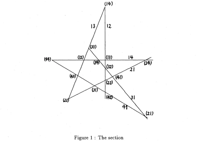
We take a hyperplane fi in $P^{3}$ which does not contain (11) and fix it. Figure 1 represents

the section by $\Pi$ of the six singular planes of$Kum(A_{\tau})$ passing through (11).

Figure 1 : The section

On each line in the figure we mark the symbol of the corresponding singular plane : 12,

13, 14, 21, 31, 41 ; on the intersection oftwo lines we markthe symbol ofthe double point, different from (11), lying on the two corresponding singular planes. Therefore, the point

Remark 3.3 Let $D$ be a curve on $Kum(A_{\tau})$, Then the projection

of

$D$

from

(11) on II

intersects to six lines in Figure 1 at$po\underline{in}ts(ij)$ or touches them because the singular plane

$H_{x}$ touches $Kum(A_{\tau})$ along the conic $\Theta_{x}$.

Proposition 3.4 There exists a conic $\Gamma$ in II which touches six lines in Figure 1.

PROOF. Consider the tangent cone to $Kum(A_{\tau})\subset P^{3}$ at the double point (11) and let $\Gamma$

be the section of it by II. Then it follows that $\Gamma$ satisfies the above condition. $\square$

We can take a homogeneous coordinate $x,$ $y,$ $z$ of II $\cong P^{2}$ such that. $\Gamma$ is given by the

equation $yz=x^{2}$ and any three among six contact points are given by

$(x ; y ; z)=(0$ ; $0$ ; 1 $)$, (1 ; 1; 1), $(0$ ; 1; $0)$.

So it may be assumed that the line 14, 21, 12, 13, 31, 41 are given by the equation

$y+2a_{1}x+a_{1}^{2}z=0$, $y+2a_{2}x+a_{2}^{2}z=0$, $y+2a_{3}x+a_{3}^{2}z=0$,

$y=0$, $y+2x+z=0$, $z=0$

respectively.

Proposition 3.5 $C$ is isomorphic to the curve given by the equation $y^{2}=x(x-1)(x-$

$a_{1})(x-a_{2})(x-a_{3})$.

Now we consider the endomorphism ring End$(A_{\tau})$ of$A_{\tau}$

.

Analytically,

End$(A_{\tau})=\{\alpha\in M_{2}(C)|\exists M\in M_{4}(Z)$ s.t. $\alpha(\tau 1_{2})=(\tau 1_{2})M\cdot\cdot(*)\}$. Let $M=(\begin{array}{ll}A BC D\end{array})$ . Then we have that

$(*)\Leftrightarrow\tau B\tau+D\tau-\tau A-C=0\cdots(**)$

.

We let $E$be the Riemannform associated to the polarization O. $E$defines aninvolution on End$(A_{\tau}),$ $\alphaarrow\div\alpha^{o}$, called the Rosati involution. It is determined by_{$E(\alpha z, w)=E(z, \alpha^{o}w)$}

for all $z,$ $w\in C^{2}$

.

We have that

$\alpha^{Q}=\alpha\Leftrightarrow A={}^{t}D,$ $B=(\begin{array}{ll}0 b-b 0\end{array}),$ $C=(\begin{array}{ll}0 c-c 0\end{array})$ .

Put $A=(\begin{array}{ll}a_{1} a_{2}a_{3} a_{4}\end{array})$. Under the assumption $\alpha^{O}=\alpha$, it follows that

$(**)\Leftrightarrow a_{2}\tau_{1}+(a_{4}-a_{1})\tau_{2}-a_{3}\tau_{3}+b(\tau_{2^{2}}-\tau_{1}\tau_{3})+c=0$

.

Then

Tr $\alpha=a_{1}+a_{4}$, $\det\alpha=a_{1}a_{4}-a_{2}a_{3}+bc$.

So the discriminant of the characteristic polynomial of$\alpha$ is

Definition

3.6 (Humbert [7]) For an element $\tau=(\begin{array}{ll}\tau_{1} \tau_{2}\tau_{2} \tau_{3}\end{array})$

of

$\mathfrak{H}_{2}$, it is said that $\tau$

has a singular relation with invariant $\triangle$

if

there exists an element $(a, b, c, d, e)(\neq 0)\in Z^{5}$

such that:

1. $a,$ $b_{i}c,$ $d,$ $e$ are relatively prime

2. $a\tau_{1}+b\tau_{2}+c\tau_{3}+d(\tau_{2^{2}}-\tau_{1}\tau_{3})+e=0$

3. $\Delta=b^{2}-4ac-4de$_.

As we have stated above, asingular relation of$\tau$ withinvariant $\triangle$ corresponds to

endomor-phisms of$A_{\tau}$ fixedby the Rosati involution such that the discriminant of their characteristic

polynomial is $\triangle$. Define

$N_{\Delta}=\{\tau\in \mathfrak{H}_{2}|\tau$ has a singular relation with invariant $\triangle\}$

and

$H_{\Delta}=image$ of$N_{\Delta}$ under the canonical map $\mathfrak{H}_{2}arrow Sp(4, Z)\backslash \mathfrak{H}_{2}$

where $Sp(4, Z)$is the symplecticgroup over $Z$ and $Sp(4, Z)\backslash \mathfrak{H}_{2}$ denotes the quotient space

for the well known $ac$tion. $H_{\triangle}$ is called the Humbert surface of invariant $\triangle$. The following

result, which is stated explicitly in [2], p.212, is essentially due to Humbert:

Proposition 3.7 Each point

_of

$H_{\triangle}$ can be represented by $\tau\in \mathfrak{H}_{2}$ satisfying an equation

$a\tau_{1}+b\tau_{2}+\tau_{3}=0$ with $b^{2}-4a=\Delta,$ $b=0$ _{or 1.}

Proposition 3.8 (Humbert [7])

_If

$\tau\in \mathfrak{H}_{2}$ has a relation

$-\tau_{1}+\tau_{2}+\tau_{3}=0$,

there exists a conic $D$ in $\Pi$ which passes through

five

points

(34), (14), (33), (22), (24)

and touches the line 41 (see Figure 1). Conversely,

_if

the latter holds, $\tau$ has a singular

relation with $\triangle=5$.

Using this proposition, Humbert calculated a modular equation of $H_{5}$.

Theorem 3.9 (Humbert [7]) there exists a conic in $\Pi$ which

satisfies

the conditions in

Theorem 3.8

_if

and only

_if

the identity

4$(a_{1}^{2}a_{3}-a_{2}^{2}+a_{3}^{2}(1-a_{1})+a_{2}-a_{3})(a_{1}^{2}a_{2}a_{3}-a_{1}a_{2}^{2}a_{3})$

$=$ $(a_{1}^{2}a_{3}(a_{2}+1)-a_{2}^{2}(a_{1}+a_{3})+a_{2}a_{3}^{2}(1-a_{1})+a_{1}(a_{2}-a_{3}))^{2}$

Humbert $al$so calculated a modular equation of$H_{8}$.

Proposition 3.10 (Humbert [7])

_If

$\tau\in \mathfrak{H}_{2}$ has a relation

$-2\tau_{1}+\tau_{3}=0$,

there exists a curve

_of

degree 4 and genus 1 in$Kum(A_{\tau})$ which passes through double points

(32), (34), (42), (44).

Projecting

_from

(11) on II, there exists a conic in $\Pi$ which passes through the

four

points

in $\Pi$ corresponding to the above double points and touches the line 21 and 13. Conversely

if

such a conic exists in II, $\tau$ has a singular relation with $\triangle=4$ or 8.

Theorem 3.11 (Humbert [7]) Consider a conic $y=x^{2}$ and its six tangents

$l_{\delta}$ : $y+2\delta x+\delta^{2}=0$,

$\delta=\infty,$ $0,$ $b_{1},$ $b_{2},$ $b_{3},$ $b_{4}$. Then there exists a conic which passes through the

four

points

$l_{b_{1}}\cap l_{b_{2}}$, $l_{b_{2}}\cap l_{b_{3}},$ $l_{b_{3}}\cap l_{b_{4}},$ $l_{b_{4}}\cap l_{b_{1}}$

and touches $l_{\infty}$ and $l_{0}$

if

and only

if

the identity

$(b_{1}b_{3}-b_{2}b_{4})^{2}-\cross$

$(4b_{1}b_{2}b_{3}b_{4}((b_{1}+b_{3})(b_{2}+b_{4})-2b_{1}b_{3}-2b_{2}b_{4})^{2}-(b_{2}-b_{4})^{2}(b_{1}-b_{3})^{2}(b_{1}b_{3}+b_{2}b_{4})^{2})=$

holds. Moreover, the

_{first factor}

corresponds to $\triangle=4$ and the latter corresponds to $\triangle=8$.

4

Modular

embedding of

quaternion

algebras with

$D=6$

and

10

4.1

The

case

of

$D=6$

Let

$B_{6}=Q+Qi+Qj+Qij,$ $i^{2}=-6,$ $j^{2}=2,$ $ji=-ij$

be the quaternion algebra over $Q$ with discriminant 6 and let

$\mathcal{O}_{6}=Z+Z\frac{i+j}{2}+Z\frac{i-j}{2}+Z\frac{2+2j+2ij}{4}$

be a maximal order of $B_{6}$. Put $\rho_{1}=i$ and consider an involution on $B_{6},$ $\alpha\alpha^{*}$ $:=$

$\rho_{1}^{-1}\alpha’\rho_{1}$, where ’ is the canonical involution on $B_{6}$. Then it holds $\mathcal{O}_{6}^{*}=\mathcal{O}_{6}$. Since $\rho_{1}^{2}=$

$-6<0$, it is positive : $Tr(\alpha\alpha^{*})>0$ (if$\alpha\neq 0$) where Tr denotes the reduced trace of $B_{6}$

It is known that the complex upper half plane $\mathfrak{H}$ can be embedded into $\mathfrak{H}_{2}$ by using

$(B_{6}, O_{6}, \rho_{1})$. We shall state this process. We fix an isomorphism$bfB_{6}\otimes_{Q}Rarrow M_{2}(R)$

given by

$i(\begin{array}{ll}0 -16 0\end{array})$ , $j(\sqrt{2}0-\sqrt{2}0)$

and identifying them. For an element $z\in \mathfrak{H}$, we define the map

$f_{z}$ : $B_{6}\otimes_{Q}Rarrow C^{2},$ $\alpha\alpha(\begin{array}{l}z1\end{array})$ .

Put $D_{z}=f_{z}(\mathcal{O}_{6})$

.

It follows that $D_{z}$ is a lattice in $C^{2}$

.

Define a pairing

$E$ : $D_{z}\cross D_{z}arrow Z$

by $E(f_{z}(\alpha), f_{z}(\beta))=Tr(\rho_{1}^{-1}\alpha\beta’)$. It is well known that $E$is an alternatingRiemann form

on $T_{z}$ $:=C^{2}/D_{z}$

.

So $T_{z}$ is an abelian variety. By selecting a symplectic basis of $D_{z}$ and

changing the coordinate of $C^{2},$ $T_{z}$ is isomorphic to $C^{2}/<(\Omega(z)1_{2})>where$

$\Omega(z)=(-\frac{3\sqrt{2}}{4}z-\frac{1}{2}-\frac{\sqrt{2}}{8z}\frac{3}{2}z-\frac{1}{4z}$ $- \frac{3\sqrt{2}}{4}z-\frac{1}{2}-\frac{\sqrt{2}}{8z}\frac{3}{4}z-\frac{1}{2}-\frac{1}{8z})\in \mathfrak{H}_{2}$.

and $<(\Omega(z)1_{2})>=L_{\Omega(z)}$. Thus we get an embedding $\Psi$ : $\mathfrak{H}arrow \mathfrak{H}_{2},$ $z\Omega(z)$. It is

easy to check the lemma:

Lemma 4.1.1 $\Omega(z)$ has two singular relations:

$-\tau_{1}+2\tau_{3}+1=0$ with $\Delta=8$,

$\tau_{2}-\tau_{3}+(\tau_{2^{2}}-\tau_{1}\tau_{3})-1=0$ with $\Delta=5$.

On the other hand, the following theorem is well known:

Theorem 4.1.2 (Shimura) Let $A$ be a principally polarized abelian variety

of

dimension

2 such that

1. End$(A)\supseteq \mathcal{O}_{6}$

2. The Rosati involution coincides with the involution $*$

on $\mathcal{O}_{6}$.

Then there exists $a$ element$z\in \mathfrak{H}$ such that$T_{z}$ is isomorphic to$A$ asprincipally polarized

abelian variety.

By Lemma 4.1.1 and Theorem 4.1.2, we have

Proposition 4.1.3 Let $A$ be as above. Then there is $\tau=(\begin{array}{ll}\tau_{1} \tau_{2}\tau_{2} \tau_{3}\end{array})\in \mathfrak{H}_{2}$ such that

2. $\tau$ has two singular relations in Lemma 4.1.1

To combine the modular equations for $\triangle=5$ and 8, we prepare some lemmas.

Lemma 4.1.4 Let $\tau$ be an element

of

$\mathfrak{H}_{2}$ which has two singular relations in Lemma 4.1.1.

Set

$M_{1}=(\begin{array}{llll}0 0 -1 00 0 0 -11 0 1 00 1 0 0\end{array})$ , $M_{2}=(\begin{array}{lll}1 11 21 21 13 24 4-1 0-2 1\end{array})\in Sp(4, Z)$

an$d$

$\tau’=(\begin{array}{ll}\tau_{1}’ \tau_{2^{/}}\tau_{2} \tau_{3}’\end{array}):=\tau\cdot M_{1}$, $\tau^{u}=(\begin{array}{ll}\tau_{1}^{n} \tau_{2’’}\tau_{2}^{\pi} \tau_{3}^{u}\end{array}):=\tau\cdot M_{2}\in \mathfrak{H}_{2}$

where $\tau\cdot N=(\tau B+D)^{-1}(\tau A+C)$

for

$N=(\begin{array}{ll}A BC D\end{array})\in Sp$($4$, Z), Then the singular

$relation-\tau_{1}+2\tau_{3}+1=0$ is changed by $M_{1}$ to

$-2\tau_{1’}+\tau_{3}’=0(\triangle=8)$

and $\tau_{2}-\tau_{3}+(\tau_{2^{2}}-\tau_{1}\tau_{3})-1=0$ is changed by $M_{2}$ to

$-\tau_{1}’’+\tau_{2}^{u}+\tau_{3’’}=0(\triangle=5)$.

This lemma can be checked by a direct calculation. Putting $M=M_{1}^{-1}M_{2}=(\begin{array}{ll}A BC D\end{array})$,

$\tau’\cdot M=\tau$

“.

Consider the isomorphism

$\Phi$ : $A_{\tau’}$ $=$ $C^{2}/<(\tau’1_{2})>$

$=$ $C^{2}/<(\tau’A+C\tau’B+D)>arrow C^{2}/<(\tau^{u}1_{2})>=A_{\tau’’}$

induced by the mateix $(\tau’B+D)^{-1}$

.

Lemma 4.1.5 For an element

$Q= \frac{1}{2}(\epsilon_{1}\epsilon_{1}I_{\lambda_{1}^{1}\tau_{2’}^{1}+\lambda_{1}^{1}\tau_{3}^{2’}}^{\lambda\tau+\lambda’\tau},$$)$ mod $L_{\tau’}\in A_{\tau’}[2]$,

we put

$\Phi(Q)=\frac{1}{2}(\epsilon_{2}’+\lambda_{2}\tau_{2}\epsilon_{2}+\lambda_{2^{\mathcal{T}}1’’,\prime I_{\lambda_{2}\tau^{2}}^{\lambda_{2}’\tau_{3}^{u_{/}}}})$ mod $L_{\tau’’}\in A_{\tau’’}[2]$

where $\epsilon_{i},$ $\epsilon_{i}’,$ $\lambda_{i},$ $\lambda_{i}’(i=1,2)\in\{0,1\}$. Then

Theorem 4.1.6 Put

$F_{1}(X, Y,. Z)$ $=$ 4

(

$X^{2}Z-Y^{2}+Z^{2}(1-X)+(Y-Z))(X^{2}YZ-XY^{2}Z)$

$-(X^{2}Z(Y+1)-Y^{2}(X+Z)+YZ^{2}(1-X)+X(Y-Z))^{2}$

$F_{2}(X, Y, Z)$ $=$ $4XYZ((X+Y)(Z+1)-2XY-2Z)^{2}$

$-(Z-1)^{2}(X-Y)^{2}(XY+Z)^{2}$

.

Let $C$ be a curve

of

genus 2

defined

over $C$ such that $Jac(C)$

satisfies

the two conditions

in Theorem 4.1.2. Then $C$ has a model

$y^{2}=x(x-1)(x-a_{1})(x-a_{2})(x-a_{3})$ such that

$F_{1}(a_{1}, a_{2}, a_{3})=F_{2}(a_{1}, a_{2}, a_{3})=0$.

PROOF. By Proposition 4.1.3 and Lemma 4.1.4,

$Jac(C)\cong A_{\tau’’}arrow^{\Phi}A_{\tau’}$.

We shall consider on $A_{\tau’’}$

.

$C$ has a model in Proposition 3.5 for $\tau=\tau’’$. By

The-orem 3.10 there exists a curve of degree 4 and genus 1 in $Kum(A_{\tau’})$ passing through

(32), (34), (42), (44). Using Lemma 4.1.5, we see that $\Phi$ induces

{(32),

(34), (42), (44)} $arrow^{\Phi}$

{(34),

(41), (13), (22)}.

So wehave acurveof degree 4 andgenus 1 in$Kum(A_{\tau’’})$ passing through(34), (41), (13), (22).

Projecting from (11) on \ddaggerI, we obtain a conic in $\Pi$ which passes through

$14\cap 12,12\cap 21,21\cap 31,31\cap 14$

andtouches 13 and 41. Hence the second factor of the left side of the equation in Proposition

3.11 vanishes at $b_{1}=a_{1;}b_{2}=a_{3},$ $b_{3}=a_{2},$ $b_{4}=0$

.

Therefore

$F_{2}(a_{1}, a_{2}, a_{3})=0$.

On the other hand, by Theorem 3.8 and Proposition 3.9 we have

$F_{1}(a_{1}, a_{2}, a_{3})=0$

4.2

The

case

of

$D=10$ Put

$B_{10}=Q+Qi+Qj+Qij,$ $i^{2}=-10,$ $j^{2}=13,$ $ji=-ij$

$\mathcal{O}_{10}=Z+Z\frac{1+j}{2}+Z-\frac{i+ij}{2}+Z\frac{30j+ij}{13}$

and consider an involution on $B_{10},$ $\alpha-\alpha^{**}$ $:=\rho_{2}^{-1}\alpha’\rho_{2}$, where $\rho_{2}=i$. We identify

$B_{10}\otimes_{Q}R$ with $M_{2}(R)$ by

$i(\begin{array}{ll}0 1-10 0\end{array})$ , $j\mapsto(\sqrt{13}0-\sqrt{13}0)$ .

We have

$\Omega(z)=\frac{1}{13z}(1_{-360z-\frac{1-\sqrt{2}}{2}+5(1+\sqrt{2})z^{z_{2^{2}}}}80z+\frac{3-2\sqrt{2}}{4}-\frac{5(3+2\sqrt{2})}{2}$ $-360z_{1-60z-10z}- \frac{1-\sqrt{2}}{2}+5(1_{2}+\sqrt{2})z^{2})$

Lemma 4.2.1 $\Omega(z)$ has two singular relations:

$-4\tau_{1}+56\tau_{2}+12\tau_{3}+(\tau_{2^{2}}-\tau_{1}\tau_{3})+830=0$ with $\triangle=8$, $-5\tau_{1}+55\tau_{2}+15\tau_{3}+(\tau_{2^{2}}-\tau_{1}\tau_{3})+830=0$ with $\triangle=5$.

Lemma 4.2.2 Let$\tau$ be an element

of

$\mathfrak{H}_{2}$ which has two singular relations in Lemma 4.2.1.

Set

$N_{1}=(\begin{array}{llll}1 1 0 01 1 -1 117 18 -26 2731 30 -4 4\end{array})$ , $N_{2}=(\begin{array}{llll}1 1 0 01 1 1 -114 13 27 -2631 32 5 -5\end{array})$

and

$\tau’=(\begin{array}{ll}\tau_{1’} \tau_{2^{/}}\tau_{2^{/}} \tau_{3}’\end{array}):=\tau\cdot N_{1}$ , $\tau’’=(\begin{array}{ll}\tau_{1}^{u} \mathcal{T}_{2}^{//}\tau_{2}^{u} \tau_{3}’’\end{array}):=\tau\cdot N_{2}$.

Then the

_first

singular relation in Lemma 4.2.1 is changed by $N_{1}$ to

$-2\tau_{1’}+\tau_{3’}=0(\triangle=8)$

and the second is changed by $N_{2}$ to

$-\tau_{1’’}+\tau_{2’’}+\tau_{3’’}=0(\triangle=5)$.

Set

$N=N_{1}^{-1}N_{2}=(\begin{array}{ll}A BC D\end{array})$

Lemma 4.2.3 Let notations be as in Lemma 4.1.5. Then

$(\begin{array}{l}\epsilon_{2}\epsilon_{2}’\lambda_{2}\lambda_{2}’\end{array})=$

.

$(\begin{array}{llll}1 0 1 10 1 1 11 1 1 01 1 0 1\end{array})(\begin{array}{l}\epsilon_{1}\epsilon_{1}\lambda_{1}\lambda_{1}\end{array})$ .

Theorem 4.2.4 Let $C$ be a curve

of

genus 2

defined

over $C$ such that

1. End(Jac(C)) $\supseteq O_{10}$

2. The Rosati involution coincides with the involution $**$

on $\mathcal{O}_{10}$.

Then $C$ has a model

$y^{2}=x(x-1)(x-a_{1})(x-a_{2})(x-a_{3})$

such that

$F_{1}(a_{1}, a_{2}, a_{3})=F_{2}(a_{1}, a_{2}, a_{3})=0$.

PROOF.

{(32),

(34), (42), (44)} $arrow^{\Phi}$

{(23),

(12), (31), (44)} $\frac{T_{(21)}}{}$

{(34),

(41), (13), (22)}. 口

References

[1] H.-G. Franke : Kurven in Hilbertschen Modulf\"achen _{im Siegelraum. Bonner Math.}

Schriften 104 (1978).

[2] G.v.$d$. Geer: Hilbert modular surface. Springer-Verlag, Berlin, Heidelberg, 1988.

[3] R. Hartshorne : Algebraic geometry. Springer-Verlag, New York, 1977.

[4] K. Hashimoto : Base change of simple algebras and symmetric maximal orders of

quaternion algebras, Memoirs ofSci.

&Eng.

Waseda Univ., 53 (1989) 21-45.

[5] K. Hashimoto : Explicit form of quaternion modular embeddings, (preprint).

[6] R. W. H. T. Hudson : Kummer’s quartic surface. Cambridge University Press, 1990.

[7] G. Humbert : Sur les fonctions ab\’eliennes singuli\‘eres, (Euvres _{de G. Humbert 2, pub.}

par les soins de Pierre Humbert et de Gaston Julia, Paris, Gauthier-Villars (1936),

[8] T. Ibukiyama: A basis and maximal orders in quaternion algebras over the rational

number field (Japanese), Sugaku 24 (1972), 316-318.

[9] J.Igusa: Arithmetic variety of moduli for

genus

two, Ann ofMath.72 (1960), 612-649.

[10] B.Jordan : On the diophantine arithmetic of Shimura curves. Thesis, Harvard Univ.

1981.

[11] B.Jordan and R.Livn\’e : Local Diophantine properties of Shimuracurves, Math.Ann.,

270 (1985), 235-248.

[12] T.Ibukiyama, T.Katsura, and F.Oort : Supersingular curves of

genus

two and class

numbers, Comp. Math. 57 (1986), 127-152.

[13] A. Krazer : Lehrbuch der Thetafunctionen, Chelsea, New York, 1970.

[14] R.M.Kuhn: Curves of genus 2 with split jacobian. Trans. Am. Math. Soc. 307 (1988),

41-49.

[15] A.Kurihara: On some examples of equations defining Shimura curves and the

Mum-ford uniformization, F.Fac.Sci.Univ. Tokyo, 25 (1979), 277-301.

[16] F.Mestre : familles de courbes hyperelliptiques $\grave{m}$ultiplications

re\’elles,

Arithmetic

Al-gebraic Geometry, Birkh\"auser, (1991), 193-208.

[17] D. Mumford : Abelian varieties. Oxford University Press, London, 1970.

[18] M.Ohta : On $\ell$-adic representations of Galois groups obtained from certain two

di-mensional abelian varieties, J.Fac.Sci. Univ. Tokyo, 21 (1974), 299-308.

[19] G. Shimura: Introduction to the arithmetic theory of automorphic functions.

Prince-ton Univ. Press, 1971.

[20] G. Shimura : On the zeta-functions of the algebraic curves uniformized by certain

automorphic functions, J.Math.Soc. Japan, 13 (1961)

275-331.

[21] G. Shimura: Construction ofclass fields and zeta functions ofalgebraic curves. Ann.