東京藝術大学リポジトリ

(1)

Creation and Perception of

Sound Source Width in

Binaural Synthesis

Hengwei Su

Research Area of Creativity of Music and Sound

Division of Musicology and Music Studies

Tokyo University of the Arts

(2)

(3)

Abstract

Techniques able to create and control extent of sound source imagery are necessary to produce complex auditory events as usually experienced in natural auditory environment. However, methods proposed in previous study are mainly for loudspeaker reproduction. In this dissertation, a method to create source width of monophonic source in binaural synthesis is proposed. Parameters of processing and its relevant effect on perception were investigated by conducting a series of subjective listening experiments. In addition, the proposed widening processing was implemented as a DAW effect for sound effects mixing to verify its effectiveness in the application of audio production.

The approach of the processing method was to process source signals by frequency bands division and distribution to achieve widen perceived source width. The frequency components of source signals were divided into sub-bands through filterbank. The sub-bands were distributed to different directions within the range of the width which was intended to synthesize. The distribution was performed by convolution with HRTFs of corresponding directions. The influence on the perceived source width of the processing method was investigated. Three listening experiments were conducted to examine various parameters and aspects of the processing. The results showed suggested that under some conditions the widening effect can successfully create and control width for monophonic source. Method to distribute frequency bands had a significant influence on effectiveness of widening and the localizations of the width. Bandwidth of the sub-band was found to have influence on the stability of the widening effect. Furthermore, investigations of naturalness of the signals after proposed were also conducted. The results suggested that there was no severe degradation by the processing method. However, there were still limitations including individual differences and dependence on source signals, suggesting that further investigation and improvement are needed.

The overall spatial impression when using the widening effect in binaural audio produc-tion was also investigated. The result suggested that the spatial impression could be improved when using the widening effect to synthesize width for monophonic sound effects. Although the effectiveness may depended on the nature of the sound effect and the subjective criterions of the listener.

(4)

概

要

現実的に存在する音源は単純な点音源ではなく、広さ、大きさを持っている。そのため、より自然な、複雑な空間印象をもたらすため、音像を広げる処理が必_{要である。過去の音源の広がり処理に関する研究は、主にスピーカー再生を} 対象とする。そのため、この論文では、バイノーラルシンセシスにおけるモノラル音_{源の音像幅を合成する処理方法を提案した。処理のパラメータとその知覚に} 対する効果について調査するため、一連の主観聴覚実験を行った。また、提案された音_{像を広げるエフェクトをプラグインとして実装し、実際にオーディオ制作} に応用する場合に、空間印象を向上させることができるかどうかを検証した。処理のアプローチとしては、音源信号を帯域バンドの分解と分布の処理によって音_{像幅を広げる方法である。音源の周波数成分の分解はフィルタバンクに} よって行い、分解された各バンドは合成しようとする幅の範囲内に異なる方向に、_{頭部伝達関数との畳み込みで分布させた。音像を広げる処理が知覚された音} 像幅に与える影響を調査するため、三つの聴取実験を行い、様々なパラメータと側面から処理の有効性を検証した。結果により、処理が音像幅において有意な効果があり、そして音像幅とシンセシス幅との間に正の相関が見られた。それらの結_{果は、この処理方法がモノラル音源の幅を合成と制御することができると示唆} した。帯域バンドの分布方法は、音像を広げる効果と音像幅の定位に有意な効果があった。帯域幅は広げる効果の安定性に影響を与えると示した。また、処理による自然さの変化も調査した。結果により、広げる効果による顕著な劣化がなかったと示_{唆した。しかし、個人差と音源特性への依存性があり、さらに調査と} 改善する必要があると意味した。バイノーラルオーディオ_{制作に音像を広げる効果を使用する場合に、全体的} な空間_{印象について調査した。結果により、モノラルの効果音の音像幅を合成す} ることによって空間_{印象を向上させることができると考えられる。しかし、その} 効果が効果音の特性と、聴取者の主観的な嗜好による異なると示された。

(5)

4 Spatial impression of source widening effect for binaural audio production 71 4.1 Introduction . . . 71 4.2 Method . . . 72 4.2.1 Plugin Algorithm . . . 72 4.2.2 Mixing Experiment . . . 73 4.2.3 Mixing Results . . . 75 4.2.4 Stimuli . . . 75 4.2.5 Listening Experiment . . . 75 4.3 Result . . . 76 4.4 Discussion . . . 76 4.5 Summary . . . 78 5 Summary 79 References 81

(7)

Table of Contents vii

(8)

(9)

List of Figures

1.1 Research flow in this thesis . . . 3 2.1 The interaural differences . . . 7 2.2 The transfer function from the emitted position to the ear, and the transfer

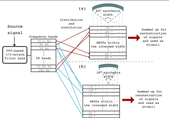
function from the source to the center of the head. . . 8 3.1 Widening processing algorithm to generate stimuli: (a) Stimulus with 60°

synthesis width, (b) Stimulus with 30° synthesis width. . . 23 3.2 1/12 octave smoothed spectrums of the three source signals. The power was

normalized so that the maximum value of each signal equals to 0 dB. . . 24 3.3 Distribution result of different distribution method for stimuli with 60°

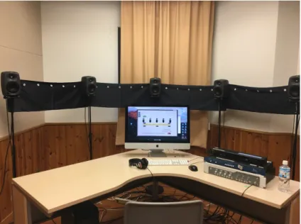
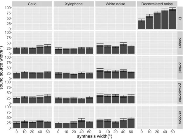
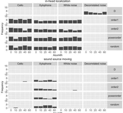
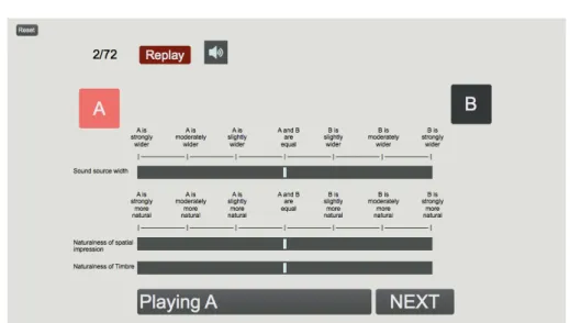
syn-thesis width. The power of each band converted to dB respecting to the maximum value of each stimuli is represented by gray gradient color. For order1, order2, and random method, the power of stimuli of cello signals is represented. . . 26 3.4 Setup of subjective listening experiment . . . 27 3.5 The GUI for perceived width evaluation. . . 28 3.6 Histogram of azimuth angles of sound source width and azimuth angles of

centers. 4 subplots from top to bottom represents different source types, panels in horizontal directions represents different synthesis widths, and panels in vertical directions represents different distribution methods. The vertical lines (red) indicate mean azimuth angles of centers of source widths. 30 3.7 How the histogram was plotted based on the reported perceived widths . . . 31 3.8 Mean source widths of different synthesis width across responses of all

participants, with error bars representing standard errors. Panels in horizontal directions represent different source types, and panels in vertical directions represent different distribution methods. . . 32

(10)

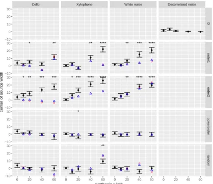
3.9 Mean center computed from experiment results (black) with error bars rep-resenting standard error, and mean center weighted by power (red circle) and A-weighting applied power (blue triangle). The significances of t-test analyzing whether the mean = 0 were marked by asterisks. . . 34 3.10 The frequencies of in-head localization and sound source moving. . . 35 3.11 GUI constructed in Cycling’74 Max for pairwise comparison in the listening

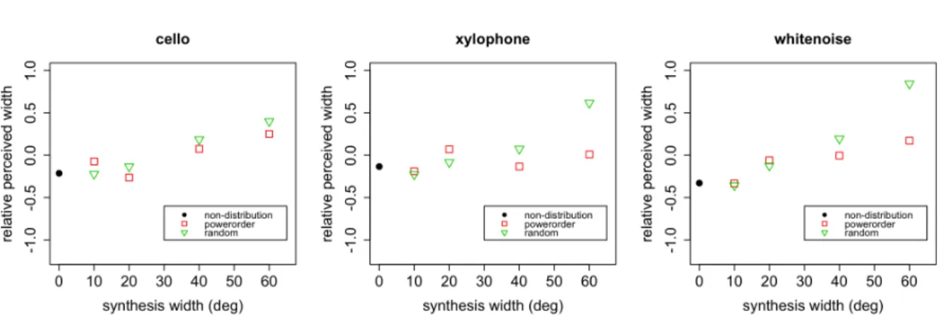
experiment. . . 40 3.12 Average relative ratings of perceived widths as a function of synthesis width

for three types of source signals. Symbols denotes different distribution method as described in the legend. . . 41 3.13 Relative perceived width as a function of 1_{−IACC and Pearson’s correlation}

coefficients between them for each source signal . . . 45 3.14 Relative ratings of naturalness from subjective listening experiments. The

upper panels are the relative naturalness of spatial attributes for cello and xylophone sources, and the lower panels represent naturalness of timbre. . . 46 3.15 Dendrogram of hierarchical cluster analysis. Height represents intergroup

dissimilarity between two groups, the number of each individual observation represent each participant. Dotted lines show how groups were divided. . . 47 3.16 Average relative perceived width for each group. . . 47 3.17 Average relative naturalness of spatial impression for each group . . . 48 3.18 Average relative naturalness of timbre for each group . . . 49 3.19 The widening processing method. (a) Stimuli with 60° synthesis width with

center at 0° azimuth. (b) Stimuli with 30° synthesis width with center at 15° azimuth. . . 55 3.20 Synthesis widths of each participants tested. Each dot indicates the synthesis

width on horizontal axis was tested by the participant on vertical axis. . . . 56 3.21 The GUI for the timbre degradation evaluation. . . 59 3.22 Mean scores for perceived width ratings of stimuli of the cello source, along

with the error bars representing standard deviations. Results for center position of 0° (left) and 15° (right) are shown respectively. . . 60 3.23 Mean scores for perceived width ratings of stimuli of the pink noise source,

along with the error bars representing standard deviations. Results for center position of 0° (left) and 15° (right) are shown respectively. . . 60 3.24 IACC of stimuli from each condition as a function of synthesis width . . . . 62

(11)

List of Figures xi

3.25 Mean scores for timbre degradation ratings of stimuli of the cello source, along with the error bars representing standard deviations. Results for center position of 0° (left) and 15° (right) are shown respectively. . . 64 3.26 Mean scores for spatial quality degradation ratings of stimuli of the cello

source, along with the error bars representing standard deviations. Results for center position of 0° (left) and 15° (right) are shown respectively. . . 65 4.1 The processing algorithm of the widening effect plugin. The example is for

the parameter of sound source width set to 30° and the sound source center set to 15°. . . 72 4.2 The interface of source widening plugin. . . 73 4.3 The setting for the mixing experiment. . . 74 4.4 GUI constructed in Cycling’74 Max for the subjective listening experiment. 76 4.5 Box plot of the ratings for each stimulus . . . 77

(12)

(13)

List of Tables

2.1 Example of statements of 7-point scales . . . 18 3.1 Statements of 7-point scales for the width evaluation and the naturalness

evaluations. . . 39 3.2 ANOVA table of width ratings for cello source . . . 41 3.3 Stimuli pairs with significant differences for cello source. * represents a 0.05

and ** represents a 0.01 significance level. . . 42 3.4 ANOVA table of width ratings for xylophone source . . . 42 3.5 Stimuli pairs with significant differences for xylophone source. * represents

a 0.05 and ** represents a 0.01 significance level. . . 43 3.6 ANOVA table of width ratings for white noise source . . . 43 3.7 Stimuli pairs with significant differences for white noise source. * represents

a 0.05 and ** represents a 0.01 significance level. . . 44 3.8 Analysis of Covariance Table for cello source with 0° center position . . . . 61 3.9 Analysis of Covariance Table for cello source with 15° center position . . . 61 3.10 The results of regression analysis. . . 63 3.11 Pearson correlation coefficient between 1_{− IACC and ratings of perceived}

widths for each participant under four conditions. The coefficients >0.5 are emboldened. . . 64 3.12 Analysis of Covariance Table of timbre degradation ratings for cello source

at 0° center position . . . 65 3.13 Analysis of Covariance Table of timbre degradation ratings for cello source

at 15° center position . . . 65 3.14 Analysis of Covariance Table of spatial quality degradation ratings for cello

source at 0° center position . . . 66 3.15 Analysis of Covariance Table of spatial quality degradation ratings for cello

(14)

4.1 Values or ranges of values of the sound source width parameter of each sound effect used by the two participants. . . 75

(15)

Nomenclature

Roman Symbols

a_i azimuth angle in degrees of the band distributed to C common transfer function

∗ convolution operator

y_l(t), yr(t) signals measured at the entrance of the left and right ear canals

E_R, HL transfer functions from the position of emitted sound to the right and left ears

H_R, HL head related transfer functions of right and left ears

max maximum value p_i power of each band s(t) monophonic source signal

(i, j) comparison pair in Scheffé pairwise comparison

x_{i jk} corresponding value of the score for the kth judge for(i, j) pair in Scheffé pairwise comparison

x_it the tth observation of covariate under ith level in analysis of covariance

Y_ε “yard-stick” for the confidence interval of αi− αjin Scheffé pairwise comparison

Y_it the tth observation of dependent variable under ith level in analysis of covariance Greek Symbols

αi, αj main effects of i and j in Scheffé pairwise comparison

ˆ

(16)

β the slope of covariate in analysis of covariance

ε error probability of the confidence interval in Scheffé pairwise comparison εit error in the model of analysis of covariance

µ represents the grand mean in the model of analysis of covariance

µi j the mean preference for i over j when presented in the order(i, j) in Scheffé pairwise

comparison

πi j the average preference for i over j in Scheffé pairwise comparison

ˆ

πi j the estimate of πi j in Scheffé pairwise comparison

τ time lag

τi the effect of ith level of the categorical independent variable in analysis of covariance

Subscripts

L, R left and right channels of the ears Style/Formatting

italic is used to indicate it a name of a database, or a name of a distribution method, evaluation term, or parameter used in experiments.

Quotation mark is used for emphasis and to indicate the first use of a term. Abbreviations

ADM audio definition model ANCOVA analysis of covariance ANOVA analysis of variance VR augmented reality

ASW apparent source width or auditory source width BRIR binaural room impulse response

(17)

Nomenclature xvii

HpTF headphone transfer function HRIR head-related impulse responses HRTF head-related transfer function

IACC interaural cross-correlation coefficient IHL in-head localization

ILD interaural level difference IPD interaural phase difference ITD interaural time difference OBA object-based audio

STFT short-time Fourier transform VR virtual reality

(18)

(19)

Chapter 1 Introduction

Binaural technique, which involves direct control of signals transferred into both ears of listeners, not only can solve the problem of spatial impression of headphone reproduction, but also has the ability to provide realistic auditory experiences, especially in the aspect of the 3D spatial acoustic reproduction [10]. Head-related transfer functions (HRTFs) encapsulate transmission properties from sound sources to a listener’s ears and contain important perceptual spatial information. Thus, incorporating HRTFSinto input signals sent

directly into ear canals can achieve authentic reproduction of an acoustic space. Binaural synthesis, which virtualizes sound objects by convolving HRTFs, can provide more flexibility and possibility of interaction than traditional methods such as dummy-head or binaural recording and virtualization of loudspeakers setup for channel-based audio. Hence, it becomes increasingly important with the development of virtual reality (VR) and object-based audio (OBA).

An HRTF usually represents transmission data of a sound source from a single direction to the ear position in the free field. As a result, simply convolving monophonic audio signals with an anechoic HRTF can produce only a perceptually point-like sound image. However, in the real world sound sources are usually not simply point sources but have extent. Hence, source widening processing for monophonic sound objects is necessary to provide a more complex and realistic acoustic spatial impression in binaural synthesis.

The fast-evolving VR technique has drew attention to 3D audio, especially in headphone reproduction. Providing auditory information can assist recognition of a virtual space and connecting auditory perception to visual can make experience more realistic. Interactive audio and auralization of virtual sources are essential elements in VR system to achieve high degrees of realism. Hence, object-based audio rendering via binaural synthesis has became an important technique for application of VR and augmented reality (AR). The audio definition model (ADM) [34], which provides a standard of metadata for next generation

(20)

audio content, for object-based format includes parameters related to source extent such as width, depth, and height. Thus, techniques for object-based audio rendering capable of expressing those parameters are demanded.

Among the attributes related to localization or the shape of sound objects, spatial extent is an important aspect of the overall spatial impression due to the strong ability of our auditory system to perceive the lateral size of the source. Auditory perception of spatial extent has been investigated in various fields such as room acoustics and audio production. For perceived source extent of a direct sound without reflections, research basically investigated the effect of frequency-dependent decorrelation or panning. Nevertheless, previous studies about source widening processing were mainly for loudspeaker reproduction. This study thus focuses on the perceived source width in headphone reproduction and source widening processing methods for binaural synthesis.

1.1 Aims and Scope of the Thesis

This dissertation aims to propose a method to control the source width in binaural synthesis. With the implementation of an approach of frequency band decomposition and spatial distribution to binaural synthesis, the effectiveness of widening processing was verified, and influences of the parameters of the processing on perceived source width were examined. Besides, the other aim is to investigate the effect of the widening processing on the spatial impression in the practical application of audio production.

In this dissertation the scope is in the synthesis and the perception of the width, which is the width produced by the direct sound, i.e. the sound source itself in the absence of room reflections. Also, only the lateral size of the sound is within the scope of this thesis.

1.2 Organization of the Thesis

The research flow and the organization of this thesis is displayed in Fig. 1.1. Chapter 2 provides backgrounds related to this dissertation, including an overview of binaural technique, reviews of studies about perceived source width, and basic concepts of analysis methods used in this thesis. In Chapter 3 there experiments investigating a source widening processing method and its effects on width perception are presented. In Chapter 4, a validation experi-ment for practical application of the widening processing to audio production is presented. The study is concluded in Chapter 5.

(21)

1.2 Organization of the Thesis 3

(22)

(23)

Chapter 2 Background

2.1 Binaural Technique

2.1.1 Introduction of Binaural Technique

The concept of binaural technique is to directly control the input signals to the auditory system, i.e. the acoustic signals at the eardrums of ears. It can be defined as all recording, analysis, synthesis, reproduction techniques which involve the signals directly replayed in the entrances of both ear canals of the listener [10].

Binaural hearing, as opposed to monaural hearing, can provide much more reliable acoustic cues for cognition of audio events, especially regarding aspects of spatial perception. This is because the auditory system can process information of the differences between input signals to two ears which are at different positions in the sound field [14]. If crucial binaural cues for auditory system are captured and provided properly, realistic sound fields can be reproduced. Hence, binaural technique is especially important for applications in the field of spatial audio.

To provide backgrounds of binaural techniques relevant to the studies in this thesis, this section firstly introduces head-related transfer function, which is the most crucial part in binaural technique. Then basic concepts for recording, reproduction, and synthesis techniques for binaural audio are given. Finally methods of binaural synthesis used for rendering various audio formats are overviewed.

(24)

2.1.2 Head-Related Transfer Function

Localization Cues

The ability of humans to recognize the direction of the sound source relies on the processing of information of the sound, which is called “localization cues,” by auditory system [25]. Localization cues are classified as binaural cues and monaural cues. Binaural cues, or interaural cues, comes from comparing the differences between the two input signals at the two ears. Interaural level difference (ILD) and interaural time difference (ITD) are the two binaural cues and also considered the most important cues in horizontal plane. ITD is resulted from the difference in distances from the sound source to both ears, as illustrated in Fig. 2.1. The path to the contralateral ear (on the opposite side to the sound source) is longer than the path to the ipsilateral (on the same side to the sound source) ear, which leads to the difference in arrival times of the sound wave emitted from the sound source. Based on a simplified model assuming the geometry of the head is spherical, the ITD can be computed as following equation:

τ =r(θ + sinθ )

c (2.1)

where τ is the ITD, r is the radius of the head, θ is the azimuth of the source in radians, and cis the velocity of sound. ILD occurs due to the presence of the head of the listener, which serves as an obstacle causing attenuation of the incident sound wave. The sound pressure level at the contralateral ear is lower than the level at the ipsilateral ear. Both ITD and ILD vary depending on the incident direction of the sound, thus human auditory system can utilize the ITD and ILD to judge the direction of the sound. On the other hand, monaural cues are spatial information that can be resolved only by one ear, or the information is common to both ear. The most dominant monaural cues related to the localization of the direct sound is from the variation of spectrum of the signals depending on the incident direction of the sound, which is called “spectral cues”. Spectral cues are mainly derived from the filtering effect of the head, which will be introduced in the next section.

Head-Related Transfer Function

A Head-related transfer function (HRTF) describes transmission properties from a point sound source to a position in the ear canal of a listener in free-field. The transfer function encapsulates filtering effect of head, pinna and torso of the listener corresponding to the particular direction. Thus, HRTF not only intuitively represents binaural directional cues of ILD and ITD, but also provides monaural spectral cues for localization, which have been known as primary cues for localization of elevation [5].

(25)

2.1 Binaural Technique 7

Fig. 2.1 The interaural differences

HRTF a commonly defined as the transfer function from the source to the ear divided by the transfer function from the source to the center of the head without the head being present, i.e. H_R= ER c H_L= EL c (2.2)

where HR, HL are the HRTFs of right and left ears, ER, EL are the transfer functions from the

position of an emitted sound to the ear, c is velocity of sound, which is usually obtained by the transfer function from the source to the center of the head (Fig. 2.2). In this definition, the transfer functions of measurement apparatus, such as a microphone or loudspeaker, have been inherently compensated.

Encoding HRTFs into input signals sent directly to both ears can provide important perceptual spatial information and reproduce the acoustic space authentically. However, due to the anatomical differences of human, the HRTF varies largely between individuals. Using non-individual HRTF will cause problems such as localization inaccuracies, inside-head localization, front-back and up-down confusions, and timbral coloration [32].

Individualization of HRTF

Individual HRTFs can be acquired by direct acoustic measurements from human sub-jects [18]. Nevertheless, the measurement procedure is usually tedious and time-consuming, since specific equipment such as anechoic chamber, loudspeakers, and in-ear microphones are required, and the measurement and recalibration require a lot of time to obtain HRTFs

(26)

Fig. 2.2 The transfer function from the emitted position to the ear, and the transfer function from the source to the center of the head.

from different directions with sufficient resolution [8]. As the measurement is not always feasible for all researchers or engineers, a lot of HRTF databases of human subjects or artificial body measurements are provided by many organizations such as KEMAR – the MIT Media Lab HRTF Database[9], LISTEN – the IRCAM HRTF Database,1the CIPIC Lab HRTF Database[2], and the RIEC HRTF Dataset [37], which are all available online.

Apart from direct measurements, other methods to obtain individual HRTFs are also developed [38, 32], such as theoretical diffraction computation based on modeling the shape of head, ear, and torso with individual anthropometric data of the subject. With non-individual HRTFs from database, individualization can also be achieved through subjective selection, tuning, or matching according to similarity of anthropometric data.

Subjective selection is an easy and fast way to achieve individualization. Seeber and Fastl [30] presented a subjective selection method in which a two-step procedure was used to single out an optimal HRTF set. In the selection procedure, white noise pulses positioned at_{−40°, −20°, 0°, 20°, and 40° in the frontal horizontal plane by filtering with} non-individual HRTFs were used. Multiple criteria relating to localization, externalization, and front-back confusion were provided for the selection. The results showed that the selection procedure could lower the variance of the localization responses, the number of inside-the-head localizations, localization error, and the number of front-back confusions.

However, if the size of HRTF catalogue is large, the selection procedure can become tedious. To obtain a suitable number of HRTF sets for subjective selection, Tama et al. [33] used k-means cluster analysis to obtain a subset of HRTF sets with maximal differences

(27)

as the best representative from a database. The impulse responses for both ears at two positions (0° and 180° azimuth, 0° elevation) from 62 subjects were used as data for analysis. The algorithm of k-means cluster analysis was as follows: First, k centers were tentatively determined for k clusters and each data point was assigned to the cluster with the nearest center. Then each center was recalculated as the average of the data points within the cluster, and reassignment of data and recalculation of centers were iterated. In their study, the index of the data nearest to each center was recored, and when k= 5 the results showed consistent indices after 1000 iterations. Thus, a subset of 5 HRTF sets was used for the subjective selection. The result of the listening test indicated that subjects who were offered a choice of HRTF had better front-back discrimination than subjects assigned an arbitrary HRTF. These studies suggested that by conducting subjective selections with a suitable size of HRTF catalogue, HRTF individualization can be achieved in some degree with good perceptual qualities while the time cost is low and the procedure is simple.

2.1.3 Binaural Recording, Synthesis, and Reproduction

Binaural Recording

Binaural recording is based on the concept that if the two input signals recorded in the ear canals of a listener are reproduced at the same positions, the listener can be provided with all information of the sound scene, the same as the listener would receive when in the real auditory experience [10]. Instead of a real listener, an artificial body, or a “dummy head” which simulates the human body shape with the relevant acoustical properties, is more often used for convenience. Usually a dummy head is equipped with two in-ear microphones, and the binaural signals can be directly recorded by placing it in the presumed listening position. However, for most cases the listener is not the same person used for recording or the dummy head usually just represents an “average listener.” As a result, differences in HRTFs lead to inter-individual variances in the quality of binaural reproduction. Moreover, generally the recording is suitable only for headphone reproduction. For loudspeaker reproduction further processing is necessary.

Binaural Synthesis

HRTF characterizes the filtering of incident sound wave caused by the head and torso of the listener, which serves the same function of the human or the dummy head in the binaural recording. Hence, instead of recording with a physical head, binaural signals can also be generated by filtering an original signal with HRTFs. This method is called “binaural synthesis.” The filtering is usually conducted by convolution with head-related impulse

(28)

responses (HRIRs), which are the time-domain representation of HRTFs. The operation can be expressed by the following equations:

BinauralSignalL= s(t)∗ HRIRL

BinauralSignalR= s(t)∗ HRIRR

(2.3)

where_{∗ mark stands for the convolution operator, s(t) is a monophonic source signal, and} subscripts L and R represent left and right channels of the ears. As HRTFs of all possible directions are available, the directions of virtual sound sources can be controlled by using the corresponding HRIR [35].

Binaural synthesis has many advantages over binaural recording. For example, it provides more flexibility, since for different listeners different HRTFs can be used for synthesis such as individual HRTFs. Furthermore, with dynamic synthesis, updating the HRTF according to the change of direction of sound incidence due to the head movement is possible, which is closer to natural listening and can resolve front-back confusions [1]. Nowadays, binaural synthesis techniques have been widely developed and used in many applications, such as communication systems, virtual surround sound headphones, and virtual reality. Methods for generating binaural signals from common audio formats in audio engineering using binaural synthesis are introduced in the following section.

Binaural Reproduction

The binaural signals are usually reproduced via headphones, since the signals of the left and right channels can be replayed separately to the corresponding ears, and the listening environment can be isolated to achieve a better control of reproduction. However, non-flat headphone frequency response and acoustic coupling with listener’s ears leads to spectral coloration. Thus, the equalization is necessary for authentic synthesis of binaural signals [10]. The headphone transfer function (HpTF) can be measured at the blocked ear canal and compensated for by inverse filtering. Nevertheless, acquisition of HpTF is tedious since it also varies with individual morphology and is very sensitive to headphone repositioning. Also, proper design of the equalization filters is also required to fulfill perfect compensation [28]. As opposed to headphone reproduction, if binaural signals are reproduced via loud-speakers, the left channel of the binaural signals transmits not only to the left ear but also to the right ear of the listener, and does as the right channel. This phenomenon, which is called “cross-talk,” deteriorates authenticity of binaural reproduction and distorts spatial impression. In order to cancel cross-talk, an inverse filter to compensate for the transfer function between the contralateral loudspeaker and the respective ear can be applied [26].

(29)

This is called “transaural systems”. Recent development of transaural system is focused on solving problems such as small listening area, adaptation with head-movements, and the affect of reflections and reverberations of the room.

2.1.4 Binaural Auralization of Channel-based, Object-based, and

Scene-based Audio

Binaural synthesis is an essential part of the technique of “auralization,” which is a term to describe the technique to create audible signals with numerical data, such as room acoustic modeling and virtual auditory display [36]. Auralization of various audio formats to binaural signals, i.e. “binauralization,” or binaural rendering, becomes increasingly demanded with the rapid development of 3D audio and virtual reality.

Binauralization of Channel-based Audio

Binaural synthesis was firstly widely applied for replaying the channel-based audio on headphone. Since stereophonic audio was originally created for loudspeaker reproduction, reproducing it directly with two channels of headphones distorts the sound scene and causes inside-head localization. To solve these problems, the loudspeaker setup, usually at_−30° and 30° azimuth for stereophony, can be simulated by convolving channel signals with HRTFs of the directions of virtual loudspeakers. By doing this, the signal of each channel is reproduced as if from the corresponding virtual loudspeaker in the direction of the HRTF. Besides stereophony, virtualization of loudspeakers can also be applied to multichannel loudspeakers layout such as 5.1ch [22] or 7.1.4 [6] channel systems. This virtual surround technique can create 3D surround sound with just 2 channel headphone reproduction, and has attracted much attention and been commercialized for applications such as home theater system.

However, virtualization of loudspeakers to render channel-based audio inevitably suffers from problems occurred when using nonindividual HRTFs, which is usually the case for commercial audio. With timbre colorization and insufficient improvement in spatial impres-sion such as lack of externalizaion, many studies report that listeners preferred original stereo or down-mixed stereo versions over binauralized versions. Using binaural room impulse responses (BRIRs) instead of HRTFs measured in the free-field is known to improve the timbre and provide better impression since the experience closer to that when listening to loudspeakers in a room [6]. BRIRs are HRIRs measured in a listening room, so early reflections and reverberation of the room are all so included in the impulse response, or these components can be added through room simulation.

(30)

Binauralization of Object-based Audio

Instead of reproducing channel-based signals by virtual speakers, recently developed object-based audio (OBA) provides an alternative approach to auralization sound scene into binaural signals. In OBA, as opposed to transmitting a set of channel signals which are specified for a particular loudspeaker setup, a set of sound objects and their metadata are transmitted. Those sound objects constitute a sound scene based on the metadata describing the attributes of sound objects such as spatial position and playback level. The rendering is done at the reproduction end according to the given reproduction setup to ensure that the spatial impression will not distort and can be optimized for different reproduction systems and listening environments. Hence, OBA format is independent of the reproduction platform [31]. Due to these benefits, OBA is considered an important format for future spatial audio distribution.

Binaural rendering of OBA can be done by directly convolving individual source signals of sound objects with HRTFs based on the position metadata. Directly virtualizing each sound object of a sound scene individually not only provides better spatial impression and more natural auditory experience, but also provides more flexibility and enables interaction. Hence, it is promising for applications in game audio, broadcast, and virtual reality, in which interactive experience is important.

Binauralization of Scene-based Audio

Ambisonics is a scene-based audio format which is also independent of reproduction sys-tems, since its sound field is encoded by spherical harmonics and can be decoded according to loudspeaker setup [3]. With the development of ambisonics microphones, which can capture a sound scene in 3D representation, it has achieved popularity in 3D audio applications, espe-cially in virtual reality. Binaural rendering of scene-based audio for headphone reproduction can be done by virtual loudspeakers as described above by firstly transforming Ambisonics format to loudspeakers feed and convolving those signals with HRTFs corresponding to loudspeakers positions.

2.2 Sound Source Width

In acoustic research many theories or models simplify sound sources as point sources. For example, an HRTF simply describes a transfer function from one source point to the point of an ear cannel of the listener. However, in real life sound sources are usually not point sources but have extent due to the physical size and radiation pattern of the source. In

(31)

2.2 Sound Source Width 13

addition, the “perceived” source extent, i.e. the size of the sound image in auditory space of the listener as opposed to the size of the “real” source, also increases due to room reflections.

The extent is an important attribute and has a significant influence on the overall spatial impression [15]. Perception of the extent of a sound in auditory space has been studied in various areas from different aspects and in different definitions. In this thesis, only extent of one single source in the horizontal direction, that is, “sound source width” is discussed. This section firstly introduces the perception of sound source width, after which studies related to source widening effects are reviewed.

2.2.1 Auditory Perception of Extent

Although extent is usually thought as a localization-related attribute, the definition and perception of sound source width is more complicated than the “localization” attribute, which has absolute or specific values and definition and can be referenced to a real space with other perceptual dimensions such as vision. It has been well-established that auditory extent is related to frequency, intensity level, and temporal duration of a signal [20]. Perceived extent of a sound increases as the level or duration increases, and decreases as the frequency increases. It has been assumed to have connections with the experience in our daily life when encountering with naturally occurring acoustic sources, as sound sources with bigger size usually produce a higher-level, lower-frequency, longer-duration sounds. Thus, perception of extent is usually considered a “learned attribute,” which means it is a relative and subjective impression of space like other spatial attributes, e.g. envelopment, spaciousness, reverberance and presence, which vary with individual apprehension.

In addition to frequency, level and duration, which are difficult to alter without changing other aspects of perception of sounds, the interaural difference in binaural hearing also has influence on the perceived width of the sound. There has been extensive research regarding the relationship between correlation, i.e. the similarity, between two input signals to the two ears and the perceived extent of the sound. Perrott and Buell [20] found that two uncorrelated noises replayed at two channels of headphones produced a sound image with size bigger than that of correlated noises. Kendall [13] proposed a method to create decorrelated signals and discussed its effects on spatial impression of the sound image. The term decorrelation means to process an audio source signal to lower the correlation with the original signal by transforming the waveforms, while maintaining certain aspects of the signal so that it still sounds the same as the original. By a pair of all-pass filters with random phase responses, a pair of decorrelated signals can be produced. One of the effects of decorrelation was stated that with two signals reproduced by stereo loudspeakers, the image width increases as the correlation decreases. The correlation can be statically described by the measure of interaural

(32)

cross-correlation coefficient (IACC), which is the maximum absolute value of the normalized cross-correlation function between two ear signals:

IACC= max Rt₂ t1 yl(t)yr(t + τ)dt q Rt₂ t1 y 2 l(t)dt Rt₂ t1 y 2 r(t)dt for_{− 1ms < τ < +1ms} (2.4)

where y_l(t) and yr(t) represent signals measured at the entrance of the left and right ear

canals, and τ is the time lag, which corresponds to the ITD when the maximum value is obtained [14]. Time lag between 1 ms and +1 ms is usually used based on the ITD of a completely lateral sound considering the size of the human head. It has been found that there is an inverse relationship between the IACC and perceived source width [16, 4].

In the field of concert hall acoustic, auditory perception of width has been extensively studied to develop a model to predict perceived source width based on IACC or other parameters [39]. In this context, usually a term of apparent source width (ASW, or auditory source width) is used instead, which describes the phenomenon that the perceived extent of the sound source is broadened to exceed its actual physical size due to the influence of early reflections. When a listener receives the direct sound and the reflections, which are mostly from directions different from the direct sound, the auditory system recognizes those sounds as one auditory event as long as the time delay is within certain thresholds. That is, sounds from different directions fuse together as one diffuse, or broadened, sound image. This “fusion” phenomenon also happens in the precedence effect [14].

However, even when the reflections of the room are absent, a sound source can still be perceived as having extent. Many sounds in the natural world, such as those made by leaves on a street blown by the wind, a piano, or the seashore sound, do not radiate like point sources and can be perceived as substantially extended. Due to the physical size of the source, multiple parts or positions of the source would radiate similar but not identical sounds. As long as those sounds share similar characteristics, they can be perceived as one sound source although they come from different directions.

2.2.2 Perceived Source Width in Audio Reproduction and Sound Source

Widening Effect

If identical signals come from different directions, such as emitted from loudspeakers at different positions, those signals are summed up when arriving ear canals and would end up producing a “averaged” directional cue. In this situation, usually only a narrow sound image is produced at the center of gravity of those loudspeakers according to gain factors. This is

(33)

2.2 Sound Source Width 15

how phantom source be generated in the amplitude panning of loudspeaker reproduction. It can also be interpreted as HRTFs of directions those identical signals from are averaged to rebuild a HRTF corresponding to the position of the phantom source, which is often called “summing localization” [3]. This is similar to the idea for HRTF interpolation using the method of computing a weighted average of two or more neighboring HRTFs [8]. On the other hand, if incoherent signals are emitted from loudspeakers at different positions, a spread sound image can be produced, until the coherence is too low that the auditory event disintegrates to separate sound images.

Based on this concept, Potard and Burnett [23, 24] used decorrelation to produce multiple uncorrelated point sources signals replayed by multichannel loudspeakers to control the perception of sound source extent. The results showed that sources with different extent could easily be perceived and discriminated by listeners. In addition, they proposed a method to alter the decorrelation in different frequency bands, which basically produces sources with frequency bands perceived in different positions with different spatial extents.

Deccorelation is also widely used in the traditional pseudo-stereo techniques to produce a widened sound image when replaying a monophonic signal via stereo loudspeakers. Zotter and Frank [40] proposed filter pairs to generate decorrelated signals and investigate such performance for phantom source widening in stereo loudspeaker reproduction. The filter algorithms are either phase or amplitude-based, introducing frequency-dependent differences in pairs of loudspeaker signals following a sine or cosine function. As opposed to random-phase Fourier-based FIR, such as the method proposed by Kendall [13] described in the previous section, these filters are deterministic, so can generate stable results to investigate the relationship between parameters, acoustic attributes, and perceived source width. By adjusting parameters these two filter implementation can control IACC, which has been shown to have correlation with perceived source width in previous results of listening tests [42]. This type of decorrelation method can also extend to multichannel filters and to application in Ambisonics format [41].

It should be noted that manipulating phase or amplitude spectrum is actually a kind of frequency-dependent panning to produce different IPD (interaural phase difference) or ILD in different frequency bands. However, the approach of decorrelation is usually known to suffer from the problem of spectral coloration.

Hirvonen and Pulkki [11] studied a different but similar approach by using bandpass noises in various frequency bands presented via different loudspeakers of a loudspeaker array from _{−22.5° to 22.5° azimuth on the horizontal plane to investigate the center of sound} image and the perceived width. The results of listening test showed that the perceived width was less than half the actual width for all test cases, suggesting that frequency bands from

(34)

different loudspeakers were perceived as fused together spatially. The stimuli used in their study can also be interpreted as broadband noises with directional cues, such as ITD and ILD, suggesting different localizations at different frequency bands. Signals with conflicting cues were found to produce diffuse, unsharp sound images [26].

To implement this concept as a method for synthesizing the perceived spatial extent for a monophonic input signal in auditory displays, Pihlajämaki et al. [21] revised previous explorations and established a algorithm which uses short-time Fourier transform (STFT) to decompose source signals into time-frequency bins and distribute them to loudspeakers from different directions. Different parameters related to spatial distribution and window size of STFT were examined to achieve an optimal quality of perception. Results indicated that the effect could depend on signal content and suggested that parameter tuning was required. Generally, this study demonstrated that distributing narrow frequency bands into space can create a spatially extended perception of sound source, and various distribution widths can be produced. The subjective preference and the naturalness were also investigated. The results of formal and informal listening tests indicated that this approach could maintain good timbral quality while achieving synthesis of spatial extent.

2.2.3 Source Widening Effect in Binaural Reproduction

Techniques able to create and control extent of sound sources without altering reverber-ation are necessary to produce complex auditory events as usually experienced in natural auditory environments, especially for 3D audio systems which aim to provide immersive and realistic spatial perception. However, methods described in the previous section are mainly for loudspeaker reproduction. To our knowledge there is still a lack of study about width perception or methods to control widths of sound objects in binaural synthesis, although it is necessary especially for VR applications when rendering object-based audio in binaural reproduction.

For implementation of source widening effect to binaural synthesis, an approach which distributes frequency components across different directions is intuitive and feasible. Instead of a large number of loudspeakers, which is impractical for general applications, what is required is only a set of HRTFs. The distribution can be easily done by convolving frequency components with HRTFs with proper spatial resolution, and the width and its localization can be easily controlled by utilizing HRTFs of various directions. Thus, this study implemented this approach to binaural synthesis and examined the effect on perceived source width.

The focus of this dissertation is on the widening effect and width perception of sound source itself in the absence of room reflections. Here “width” represents the spatial extent on the horizontal plane, as we focused only on the width in the frontal direction where humans

(35)

2.3 Experiment Design and Analysis Method in Psychoacoustics Research 17

are most sensitive regarding localization of sounds [17]. Since the localization mechanism of auditory system for elevation is quite different from that for azimuth, the spatial spread in the vertical direction is not within the scope of this study.

2.3 Experiment Design and Analysis Method in

Psychoa-coustics Research

Subjective listening experiment is the most common methodology in the field of psychoa-coustic research, and also frequently used for audio quality evaluation in audio engineering. In subjective listening experiment, stimuli are prepared under different conditions according to the subject of investigation, and participants of the experiment are asked to perform evaluations according to the presented stimuli, then statistical analysis is conducted based on the evaluation data.

Analysis of variance (ANOVA) and student’s t-test are frequently used analysis methods in psychological statistics to compare differences among means of two or multiple groups, such as responses under different treatments, to evaluate the effects of treatments.

In this dissertation, other analysis methods which are less commonly used are introduced.

2.3.1 Scheffé’s Pairwise Comparison

For subjective evaluation the description can be in a direct, such as ratings with regard to a certain attribute, or indirect scaling through comparison of two stimuli. Pairwise comparison, which compares two out of all stimuli at a time for all possible pairs, can provide a easier way to judge, so is suitable for circumstances when perceptual differences between stimuli is small or the absolute quantity of the perception is difficult or impossible to evaluate.

Scheffé developed a method to analyze pairwise comparison experiments [29]. In such comparison, participants not only indicate which one of a pair they prefer with regard to the respective attribute, but also evaluate the preference on a scale which can be converted to a numerical score. An example of statements for a 7-point scale when comparing a fixed order pair of(i, j) is listed in the following table, and corresponding values of the scores are also shown.

Under the mathematical model Scheffé proposed, the corresponding value of the score for the kth judgement is xi jk, the mean of xi jkfor all judgements can be used as the estimate

of µi j, which represents the mean preference for i over j when presented in the order(i, j).

(36)

Table 2.1 Example of statements of 7-point scales

statements numerical score

I prefer i to j strongly. 3 I prefer i to j moderately. 2 I prefer i to j slightly. 1 No preference. 0 I prefer j to i slightly. -1 I prefer j to i moderately. -2 I prefer j to i strongly. -3

these two means is:

πi j =

1

2(µi j− µji) (2.5)

where πi j denotes the average preference for i over j, which is

πi j = αi− αj (2.6)

where αiand αj can be considered the main effects. The estimate of αican be obtained by

the means of ˆπi j for all j.

Based on this model, sums of squares for estimates can be computed, so ANOVA can be performed. The “yard-stick” Yε is then deduced based on the variance of the estimate

ˆ

αi− ˆαj, and the confidence interval of αi− αjunder the confidence coefficient 1− ε is:

ˆ

αi− ˆαj−Yε≤ αi− αj≤ ˆαi− ˆαj+Yε (2.7)

If 0 is not included in this range, analysis suggests that the probability that there is difference between the main effect of i and j is 1_{− ε.}

In Scheffé’s method, each participant only judges only one time for a(i, j) pair in one order. This is not practical when the number of participants is small, which is the usual case for psychoacoustic experiments. For the experiment design that one participant judge all possible pairs in both orders, Ura’s variation can be used [27]. In the modified model the term of individual difference is also included.

2.3.2 Analysis of Covariance

Analysis of covariance (ANCOVA) is an analysis method based on a model which combines regression and ANOVA. ANCOVA is used when there are not only categorical in-dependent variables but also continuous inin-dependent variables, which are called “covariates.” The dependent variable is assumed to have a linear relationship with the covariate, and the

(37)

2.3 Experiment Design and Analysis Method in Psychoacoustics Research 19

differences among levels of independent variables, i.e. the “effect” of different treatments, are to be analyzed. The ANCOVA model can be written as [7]:

Y_it = µ + τi+ β xit+ εit (2.8)

where τi is the effect of ith level of the categorical independent variable, xit is the tth

observation of covariate under ith level, Yit is the tth observation of dependent variable under

ith level, εit represents error, and µ represents the grand mean. The ANCOVA model is

under the assumption that the slope of covariate β is the same for all levels of the categorical independent variable, which is called homogeneity of covariate regression coefficients, or “parallel lines model.” A statistical test of this assumption can be conducted by testing the model that slope of covariate depends on categorical independent variable, i.e. βiis used

in the model instead. If the interaction term between the categorical independent variable and covariate is significantly different from zero, regression slopes are not the same and ANCOVA should not be performed.

(38)

(39)

Chapter 3 Sound Source Widening Effect for

Binaural Synthesis

3.1 Introduction

As mentioned in the previous chapter, previous studies about perceived source width and source widening effect are mainly for loudspeaker reproduction. To propose a method to control source width in binaural synthesis, the approach which distributes frequency components across different directions as proposed in [11, 21] and described in the previous chapter, was implemented for binaural synthesis. The effects of source widening processing were investigated by conducting subjective listening experiments to investigate the perceived source width, naturalness, and spatial attributes. Parameters of the processing method were tested to investigate their influence on width perception. In this chapter, a series of three experiments conducted to achieve the above objectives is presented.

In this study, the intended source width of a monophonic sound to be synthesized, which can be controlled in the processing, is called “synthesis width.” On the other hand, the source width perceived by listeners, which is the actual target to be controlled, is called “perceived width.” In this study, the perceived width usually represents the ratings from the evaluation in subjective listening experiments.

In the first experiment, a processing method to implement frequency bands division and distribution was proposed, and the effectiveness of the processing method was investigated by directly evaluating the perceived width on the spatial coordinate. In the second experiment, an indirect ratings method was used to further examine the effect of the processing method. In the third experiment, the influence of other parameters of widening processing on the performance were also investigated, and the relationship between the synthesis width and the

(40)

perceived width was examined to verify whether the processing method can control source width effectively.

3.2 Experiment 1: Virtual source width in binaural

syn-thesis with frequency-dependent directions

In order to develop a method to control perceived width in binaural synthesis, the aim of this experiment is to verify whether the concept of distributing frequency bands of monophonic sources across different directions to achieve widened spatial extent can also be applied to binaural reproduction. Stimuli generated with different synthesis width and distribution methods were used, and subjective listening experiments were conducted to investigate the effects on the perception of source widths.1

3.2.1 Methods

Processing Algorithm of the Widening Effect for Binaural Synthesis

The processing algorithm of the widening effect for binaural synthesis is displayed in Fig. 3.1. To perform division and distribution of frequency components, source signals were firstly filtered by an FFT-based 1/3-octave filter bank. Each band was then convolved with HRTFs of directions within the intended source width range. For example, if the intended synthesis width is 60° with center at 0° azimuth on horizontal plane, the HRTFs of_−30°, −25°, −20°,. . . , 25°, 30° azimuth and 0° elevation would be used for convolution. Finally, convolved signals were summed up for reconstruction of signals which were then used as stimuli in subjective listening tests. How frequency components are distributed spatially to different directions, i.e. how each bands was assigned to different HRTF to perform convolution, is determined by various distribution methods, which is described in the next section.

Stimuli

Three types of signals — including anechoic cello recording, anechoic xylophone record-ing, and Gaussian white noise — were used as source signals. The white noise was generated by random sampling from the standard normal distribution with a duration of 10 seconds with

1_{The result of this experiment was also published in H. Su, A. Marui, T. Kamekawa, “Virtual Source Width}

in Binaural Synthesis with Frequency-Dependent Directions,” presented at the Audio Engineering Society Convention 142 (2017)

(41)

3.2 Experiment 1: Virtual source width in binaural synthesis with frequency-dependent

directions 23

Fig. 3.1 Widening processing algorithm to generate stimuli: (a) Stimulus with 60° synthesis width, (b) Stimulus with 30° synthesis width.

a 20 ms fade-in and fade-out, and normalization that the maximum absolute of samples was 0.999. The anechoic recordings were sampled from the Audio CD of Bang & Olufsen, Music for Archimedes [19]2in wave files. The duration of the cello recording was 21 seconds and that of the xylophone was 7 seconds. The 1/12 octave smoothed spectra of the three source signals are shown in Fig. 3.2.

Before processing, level alignment was performed to ensure that the loudness of three signals was perceptually the same. Three participants including the author adjusted the gain of three signals until they felt that all signals were at the same loudness. The gain could only be adjusted lower than units, i.e. lowering the level, to avoid clipping. The average values of the gains adjusted by the three participants were then used and all three participants agreed that there were no obvious misalignment of loudness among three signals. The average gain values were then applied to the three signals before processing.

HRTFs database of KEMAR dummy-head measured and provided by MIT Media Lab were used for synthesis [9]. Since this study focused only on source extent on the horizontal plane, only the HRTFs of 0° elevation were used. The synthesis widths under investigation

(42)

−60 −50 −40 −30 −20 −10 0 Cello Frequency(Hz) P o w er(dB) 16 63 250 1k 2k 4k 8k −60 −50 −40 −30 −20 −10 0 Xylophone Frequency(Hz) P o w er(dB) 16 63 250 1k 2k 4k 8k −60 −50 −40 −30 −20 −10 0 White noise Frequency(Hz) P o w er(dB) 16 63 250 1k 2k 4k 8k

Fig. 3.2 1/12 octave smoothed spectrums of the three source signals. The power was normalized so that the maximum value of each signal equals to 0 dB.

were 10°, 20°, 40°, 60°, in azimuth angles. Since the HRTF database transfer functions were measured at intervals of 5° azimuth, numbers of HRTFs used were 3, 5, 9, 13, respectively. Centers of widths for all stimuli were set to 0° azimuth, i.e. the center of the front side.

To determine which HRTF each band was assigned to, four distribution methods were applied. Identical sets of HRTFs, i.e. numbers and directions of HRTFs, were used in the four methods, but only convolved with frequency bands in different orders. 28 frequency bands, 1/3-octave bands from 20 Hz to 22050 Hz, were evenly divided to HRTFs within the range of intended width, and the remainder were assigned to HRTFs which were nearest to the center. As an example, the distribution results of four distribution methods for synthesizing 60° width stimuli are given in Fig. 3.3. The four methods were:

1. order1: The bands from low frequency to high frequency were distributed from left to right in order. Until it reached the rightmost, the distribution was repeated again from left to right in ascending order of frequency, and the remain bands were distributed as close to center as possible.

2. order2: The bands were distributed from left to right in ascending order of frequency as in the order1 method, but the higher band must be in the right position. Hence, for each HRTF there were multiple adjacent bands, and for HRTFs near center there were more bands than others.

3. random: The bands were randomly distributed to the same sets of HRTFS, but identical random patterns were used for all source types.

(43)

directions 25

4. powerorder: The bands were distributed according to the spectrum characteristics of signals, which is explained in detail following.

The forth method powerorder was adapted since in a preliminary investigation of stimuli, we found that the centers of sound images shifted to rightward, especially for the order1 and order2methods and for xylophone signal. It could be assumed as a consequence of that the frequency component of xylophone signal was almost entirely concentrated between 2 kHz to 10 kHz. The distribution methods like order1 and order2 would cause the localization of signals with narrow spectrum characteristics shifted from the center of the width (0°azimuth). Since in those methods the adjacent bands were distributed along azimuth, the bands with higher energy would focus on certain directions.

Therefore, a method that took spectral characteristics into account was also developed. The idea was that the band with higher mean power had more influence on perception, so the band with the highest power was firstly distributed to center, then the band with the second high power was distributed to_{−5°, and the third was distributed to 5°, etc. That is, the bands} were distributed with a descending order of power to HRTFs in order of proximity to center. When all HRTFs were used, the distribution started from 0° HRTF again until all bands were assigned. Consequently, the distribution results of three source types by powerorder method were different as shown in Fig.3.3, in which the gray gradient color represents the power of each band. The cello signal had rich components from 250 Hz to 700 Hz, and the xylophone signal was dominant from 2 k to 10 kHz, so those primary components were distributed near the center.

Stimuli with 0° synthesis width were also generated as references without widening processing. Source signals were convolved with 0° HRTF to synthesize sound at the 0° azimuth.

Besides stimuli described above, stimuli generated with multiple uncorrelated white noises located at different directions within intended source width ranges were also used as references. These references should be perceived with widest width, since the correlation between any pair among the signals is near 0; the perceived width of the noises ensemble should be as wide as the actual range of the directions of noise sources.

13 completely decorrelated white noises were generated by principal component analy-sis (PCA) of Gaussian white noises. Firstly, 13 randomly sampled Gaussian noises with 10 seconds duration were generated. PCA with 13 components were performed with orthogonal transformation of the 13 white noises to obtain a set of 13 linearly uncorrelated white noises. The correlation coefficients between any pair of the 13 noises after performing PCA were all on order of 10−15_{∼ 10}−17. The 13 noise sequences were then normalized so that the maximum amplitude equaled 0.999 as a safer value to avoid clipping. The spectra of 13

(44)

__ __ _____ _ ___ ___ __ _ ___ _ ___ __ −30 −20 −10 0 10 20 30 Order1 Azimuth(degree) Frequency(Hz) 31.5 125 500 2k 8k _ _ ___ _____ _ _ ____ _ ____ _ ____ _ _ −30 −20 −10 0 10 20 30 Order2 Azimuth(degree) Frequency(Hz) 31.5 125 500 2k 8k _ _ _ _ _ __ __ _ _ _ __ _ _ __ _ __ __ _ _ _ _ _ −30 −20 −10 0 10 20 30 Random Azimuth(degree) Frequency(Hz) 31.5 125 500 2k 8k 31.5 125 500 2k 8k _ _ _ _ _ _ _ _ _ _ _ _ _ _ _ _ _ _{_} _ _ _ _ _ _ _ _{_} _{_} _ −30 −20 −10 0 10 20 30 Powerorder_cello Azimuth(degree) Frequency(Hz) 31.5 125 500 2k 8k _{_} _ _{_} _ _ _ _ _ _ _ _ _ _ _ _ _ _ _{_} _ _{_} _ _{_} _ _ _ __ _ −30 −20 −10 0 10 20 30 Powerorder_xylophone Azimuth(degree) Frequency(Hz) 31.5 125 500 2k 8k _ _ _{_} _ _{_} _ _{_} _ _{_} _ _{_} _ _{_} _{_} _ _{_} _ _{_} _ _{_} _ _ _ _{_} _ _{_} _{_} _ −30 −20 −10 0 10 20 30 Powerorder_whitenoise Azimuth(degree) Frequency(Hz) 31.5 125 500 2k 8k −100 −75 −50 −25 0 power(dB)

Fig. 3.3 Distribution result of different distribution method for stimuli with 60° synthesis width. The power of each band converted to dB respecting to the maximum value of each stimuli is represented by gray gradient color. For order1, order2, and random method, the power of stimuli of cello signals is represented.

signals were examined, and all of them retained the “white” spectral characteristic with similar average power. According to the number of HRTFs within intended source width, the same number of noises were randomly chosen, convolved with HRTFs respectively, mixed and divided by root of numbers of noises to normalize the level, since when uncorrelated signals are added up the level will be root of the sum of the level.

Environment

The test was conducted in a quiet studio room with proper acoustic treatment in Senju campus of Tokyo University of the Arts. The studio room was equipped with a computer, audio interface (Avid Rack 003), and five loudspeakers. Participants were asked to use a graphical user interface (GUI) constructed in Cycling’74 Max on a computer to answer questions and perform the experiment. Stimuli were replayed via GUI through an audio interface (Avid Rack 003) and emitted by headphone (SONY MDR-CD900ST). Since participants needed to estimate perceived widths in azimuth coordinates corresponding to virtual sound sources replayed via headphone, the task could be difficult to project perceived virtual sound images into real space. Especially headphone listening often suffers from the problem of in-head localization (IHL). Hence, to facilitate the task in which participants were asked to indicate where they perceived the width of virtual sound image by answering the coordinates, five loudspeakers located at_{−60°, −30°, 0°, 30°, 60° azimuth with respect to}

(45)

directions 27

the position of the participant were used as directional references. In addition, a series of numbers to indicate azimuths in an interval of 5° was labeled on a black cloth between the loudspeakers. A photo of the setup of subjective listening experiment is shown in Fig. 3.4.

Fig. 3.4 Setup of subjective listening experiment

Procedure

The listening experiment was divided into two blocks to evaluate the perceived width and naturalnessof stimuli respectively. In the block of perceived width evaluation, participants were asked to indicate sound source widths of stimuli in azimuth coordinate, i.e., where they perceived extents of sound images. They used a bar on GUI to select the range of azimuths. The azimuth of leftmost and rightmost extent and the width of the range were shown in the GUI, as shown in Fig. 3.5. The selectable range was from_{−60° to 60° in 5° intervals.} In addition, if they perceived in-head localization and/or the localization of sound source moving while answering, they were asked to check the corresponding box to indicate that. Stimuli were played in loop so that participants were free to spend as much time as they needed for answering questions. In addition, in order to facilitate participants to answer the coordinates of virtual sound images, five reference sounds were provided. They were generated by a 500 ms white noise pulse convolved with HRTFs of_{−60°, −30°, 0°, 30°, 60°} azimuth, i.e. the directions of the loudspeaker set in the experiment room. These reference sounds virtualized the white noises reproduced by the loudspeakers which they could utilize as visual assists. Participants were instructed to use them freely, and as they click the number of azimuth presented on the GUI, corresponding sound would be replayed.