Development of the Observation system for the Jovian synchrotron radiation using an aperture synthesis array

Development of the Observation system for the

Jovian synchrotron radiation using an aperture

synthesis array

著者

Watanab Takuoe, Misawa Hiroaki, Tsuchiya

Fuminori, Miyoshi Yoshizumi, Abe Toshihiro,

Morioka Akira

雑誌名

The science reports of the Tohoku University.

Fifth series, Tohoku geophysical journal

巻

37

号

1

ページ

1-90

発行年

2005-06

Development

of the observation system for the Jovian synchrotron

radiation

using an aperture synthesis array

TAKUO WATANABE1, HIROAKI MISAWAI, FUMINORI TSUCHIYA', YOSHIZUMI IVIIYOSHI''2, TOSHIHIRO ABE' and AKIRA MORIOKA'

(Received February 17, 2005 ; accepted February 28, 2005)

Abstract : The Jovian synchrotron radiation (JSR) and its variation have important information on the acceleration, transport, and loss processes of the relativistic electrons

in the Jovian inner magnetosphere. Thus, JSR is a favorable tool for the ground-based

remote-sensing of Jovian radiation belt, which can not be obtained by in-situ observation because of the radiation damage of spacecraft. The Jovian synchrotron radiation shows

three kinds of variations ; (a) long-term (11 year), (b) medium-term (month), and (c)

short-term (days to weeks). The medium and short-term time variations are not studied

well because of the lack of continuous observation. We have developed the observation

system to attain the continuous grand-based observation of JSR. The concept of the development is to achieve the optimized and exclusive system for the JSR observation.

The system is designed to detect the Jovian synchrotron radiation with sufficient ity. The developed system consists of following 5 units ; (1) 9 antennas arranged in the Y

formation, each of which consists of 4 x 2 stacked 27-element cross Yagi antenna, (2) front-end unit with low receiver noise-temperature of about 90 K which is achieved by

using a low noise device of GaAs FET, (3) back-end whose function is to down-convert the

RF signal to IF signal, and to process the detected data, (4) loop-method calibration

system, which calibrates relative phase and gain of signal synthesizing system, and (5)

units of antenna control, communication, and personal computer system. From the performance test of each antenna and front-end unit, it was confirmed that the system noise

temperature is consistent with the value that was measured in laboratory, and that signals

from 9 antennas are suitably synthesized. Using the developed observation system, the

signal from Jupiter was successfully detected with the flux of 5 Jy, which is consistent with

previous observations. However the effective aperture area of one antenna is smaller than

the designed one. It was suggested that the roughness of alignment with 13 cm

sponding to the phase irregularity of 50°) can be the origin of the smaller aperture area.

1 Planetary Plasma and Atmospheric Research Center_{, Graduate School of Science, Tohoku} University, Sendai 980-8578

2 _{TAKUO WATANABE et al.}

1 Introduction

1.1 The giant planet Jupiter

Jupiter is the largest planet in our solar system whose equatorial radius is about 71,492 km (defined as 1R,) and heavier than the total mass of the other planets in the solar

system. Jupiter is mainly composed of hydrogen and helium gases, in common with

Saturn, Uranus, and Neptune, which are called Jupiter-type _{planet .}

Jupiter is also electromagneticaly the most active planet in our solar system. The

magnetic moment of Jupiter is 4.2 Gauss R,3 with inclination of 10° against rotation axis,

which is 20,000 times as large as that of the earth The rotation period of the Jovian

magnetic field is 9h55"29.7115 which is defined as System III rotation period , while System 1(9'5090.0034s) and System II (9'55'40.6322s) are defined as rotation period of atmosphere

near equator and pole respectively. The strong magnetic field and rapid rotation make

giant and active magnetosphere.

Moreover, Jupiter has ring and satellites near planet that interact with

magnetos-pheric plasma. The four largest satellites, Io (at 5.9R,), Europa (at 9.4R,), Ganymede (at

15.0R,), and Callisto (at 26.4R,), called Galilean satellites, interact with magnetospheric

plasma. In particular Io has a violent volcanic activity which is the origin of Io plasma

torus, and this makes Io the major plasma source of magnetospheric _{plasma . The}

Amalthea _{(at 2.5R,) which is the largest among inner moons and the Jovian ring (at}

1.7-1.8R,) is known to interact with high energy particles in the radiation belt .

As a result of the above mentioned characteristics, Jovian magnetospheric

phenom-ena are not only highly dynamic but quite different from the Earth's . The previous

in-itu and ground-ased observations have revealed unexpected phenomena such as the

violent acceleration and strong transportation of particles, powerful emission of radio

waves, and dynamic variation of plasma flow.

1.2 Radio waves from Jupiter

The magnetosphere _{of Jupiter radiates radio waves in various frequencies . Fig. 1}

shows the average Jovian radio spectrum (Kaiser, 1993). These radio waves can be

classified into thermal and non-thermal radiations and the latter can be further classified

into coherent and incoherent radiations.

Above 4 GHz (not shown in the figure), thermal radiation from the Jovian

atmo-sphere is outstanding in the spectrum which follows Plank's radiation law for the

atmospheric temperature of 135 K.

Below 100 MHz, non-thermal and coherent radiations from the Jovian polar region

are dominant. An intense decameter wavelength emission (DAM) originates in foot

print of satellite Io and To torus, and is controlled by both central meridian longitude (CML), which is the System III longitude directing to the observer, and position of Io

(Io-hase) in occurrence probability. Hectometer wavelength emission (HOM) originates in

northern and southern polar regions and has correlation _{with the solar wind .}

106- (bKOM) — (nKOM) 5"JUPITER (HOM7)10 — (DAM) — Cant.

>4

104

"\\„,

LIJ 3 10 — > kJUPITER LLI _{I (DIM)} 10 —I 1 1 EARTH t (AK R ) II 1 11 1 0.1 1.0 10 100 1000 FREQUENCY (MHz)

Fig, 1. Spectra of Jovian magnetospheric radiations. The power flux is normalized to constant distance. The spectrum of the Earth's is also shown as a comparison

with Jupiter (Kaiser, 1993).

10 torus, but the detail characteristics has not been clarified. Narrowband kilometer

wavelength emission (nKOM) is thought to have origin in the outer region of Io torus and

has the System IV periodicity (3-5% slower than system III) in occurrence periodicity.

Continuum emission has origin near the magnetopause and consists of a structure-less

component.

In the frequency range from about 100 MHz to about 4 GHz, Jovian synchrotron

radiation (hereafter referred as JSR) is emitted from the relativistic electrons, which is

a non-thermal and incoherent radiation. JSR has a flat spectrum which is mainly in the

decimeter (DIM) range (see JSR introduction in detail).

1.3 Observation history of the Jovian synchrotron radiation

In 1931, Karl G. Jansky discovered a radio emission from the Milky Way, which was

the beginning of radio astronomy (Jansky, 1933). After an interruption by the World

War II, many significant discoveries were made in 1950s and 1960s, e.g. the 21 cm line of

hydrogen, the quasars, the pulsars, and the cosmic microwave background (Burke and

Graham-Smith, 2002).

The Jovian non-thermal radiation was also discovered in this term by Sloanaker

(1959). He used an 84-foot (about 26 m) diameter parabolic antenna at a wavelength of

10 cm, and showed that apparent blackbody temperature of Jupiter is 640 K±85 K which

was unexpectedly high value comparing with infrared measurements.

As properties of the radiation (spectrum, polarization) became clear, it was thought

that the radiation is caused by synchrotron radiation originating from trapped energetic

4 TAKUO WATANABE et al.

synchrotron radiation means the discovery of extraterrestrial radiation belt by means of

the remote sensing, while the Earth's radiation belt was discovered in 1958 by Van Allen

with in-situ observation using Explorer 1.

By 1970s, static properties of JSR using single dish antenna were almost confirmed, and from which the basic properties of the Jovian magnetic field were derived such as the

magnetic field strength, polarity, tilt angle, and planetary spin period. These are

confirmed afterward by the in-situ observations _{by Pioneer 10, 11.}

After 1970s, objects of JSR observation focused on spatial distribution and time

variation to study structure and dynamics of the radiation belt . Characteristics of the

spatial distribution is described in section 2.4 in detail, while Characteristics of time

variation is described in section 2.5 in detail.

1.4 The purpose of this thesis

The Jovian synchrotron radiation reflects information on the radiation _{belt , in}

particular its time variation has an important clue to clarify acceleration and transport

processes. So far remote sensing using synchrotron radiation is the only method to

investigate the Jovian radiation belt precisely because in-situ observation is almost

impossible due to the heavy radiation damage to instruments of spacecraft _{. A few}

in-situ observation have been performed for the radiation belt, however, the observation

gave only temporal static features. We consider that it is essential to develop exclusive

observation system which enable us to make continuous observation.

In this thesis, general introduction of Jupiter is described and an introduction for JSR

is described. After summarizing _{of in-situ observation of the Jovian radiation belt , the}

basic design of the observation is described and the developed system is described

precisely. The measurements of parameters to synthesizing of signals is described, the

result of test observation is described, discussed, and concluded.

2 Characteristics of the Jovian synchrotron radiation

2.1 Mechanism of synchrotron radiation

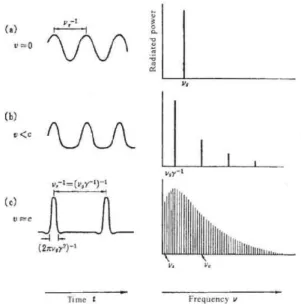
Synchrotron radiation is the relativistic counter part to cyclotron radiation. Simple

diagram of synchrotron radiation is shown in Fig. 2 (Feynman et al., 1965). For the

rotating particle with low speed, an observer looks the position of particle as sinusoidal

curve (dashed line of Fig. 2), which produces a sinusoidal electric field whose twice

derivation shows the power of electromagnetic wave. However for the rotating particle

with nearly light speed, an observer looks the position of the particle as a pulse at the

moment when the particle directs toward the observer (solid line of Fig. 2), which

produces broadband electromagnetic wave derived by the Fourier transform

of the pulse.

x'(t) 8 6 10 4 4 10 12 2 2 12 ; 0 0 _• ct observer

Fig. 2. Schematic diagram of synchrotron radiation . The observed position of a rotating particle becomes sharp at the point toward observer as speed of particle

comes to close to speed of light (Feynman, 1965).

T=-1- (1)

and the solid angle () of the radiation concerning width of the pulse is

1 (2)

where fe is the cyclotron frequency and y is the relativistic _{factor , i. e.,}

eB (3)

27rme

7= mc2 (4)

.\/114)(5)

2

The transition from cyclotron radiation to synchrotron _{radiation is shown in Fig . 3}

(reproduced from Akabane et al., 1988).

From the analytical calculation the power specta for orthogonal polarizations _{, which}

are perpendicular and parallel to magnetic field, are shown as

Pjf)=

iae3Bsin a

2c2[F(X)

G(X)]

(6)

eBsin a

11(f) ---2

mc2[F(x)—

G(x)1

(7)

respectively, where

x=f Ifc

(8)

3

f

_c=-:-272fe

₍₉₎

3e

=

47rm3c5E2Bsina

(10)

F(x)—

f1(5/3(e)ai(11)

6 TAKUO WATANABE _{et al .} yv ( a) 0 vQ

f\Ap

(b)

v<c

(\AA

_{_}

_I

I

(c)

(2x,y2)-1111111ki

Time t Frequency v

Fig. 3. Transition from cyclotron radiation to synchrotron radiation (from (a) to (c)) in the time domain (left side) and frequency domain(right side). (Adapted from

Akabane et al., 1988)

G(x)=

fK213(e)clE

(12)

K5/3 modified Bessel function of order 5/3

(13)

K213

: modified Bessel function of order 2/3

(14)

From the differences between Equation (6) and (7), it is clear that the synchrotron

radiation is polarized.

Polarization is a relationship between rectangular two

compo-nents of electric field. The Stokes parameters are convenient to display polarization of

an electro magnetic wave. The Stokes parameters are set of 4 terms defined as

I =

(15)

Q=EOcos 26'cos

2r

(16)

U=EScos2ecos2r

(17)

V =ESsin2r,

(18)

where Eo, E, and r are total power, axial ratio of polarization ecllipse, and orientation

of polarization ecllipse, respectively. The relation of these parameters are shown in

Fig. 4.

Using the Stokes parameters, degree of linear polarization (PL) and degree of

circular polarization (Pc) are displayed as

in2+ u2

P

_L

₍₁₉₎

Pc= V(20)

and degree of polarization (d) is displayed as

E0

E/Ida

p

x Polarization ellipse

Fig. 4. Relation of polarization ellipse, and definition of E and r (Kraus, 1986).

Circular polarization (right hand) Elliptical polarization (right hand)

AllAr

s4*..111W

->

linear

polarization

Elliptical

polarization

(left hand)

Circular

polarization

(left hand)

Fig.

5. Directivity of radiated power (left) and polarization (right) of synchrotron

radiation from a single electron gyrating perpendicular to the magnetic field.

d = V+ U2+ V'

(21)

= P12

_{.+ 131}

₍₂₂₎

Using Equation (6) and (7), the degree of linear polarization (PL) is derived as

PLPL(f)—Pi(f)G(x) F-L=(23)

P

L(f)+ PH(f)

Fx)

which becomes about 0.75 by integrating over all frequencies. The directivity of

radiat-ed power and polarization are shown in Fig. 5.

From Equation (6) and (7), the composed power spectrum is obtained as

P(i)=13 .1(i)+ Pli(f)

(24)

Vae

8 TAKUO WATANABE et al. 1,0 1.0

F(x)=xf:1(5,3(7;)6/27

0.5 —0.1 — _

0.1

0.01

00 0

.29 1.0

2.0

3.0

4.0 0.001

0.01

0.1 0.29 1.0

10

x=1.,/p,

x=

v/pc.

Fig. 6. Theoretical spectrum of synchrotron

radiation from a single particle, which

is displayed as Equation (11),

in linear scale (left) and log scale (right) (Akabane

et al., 1988).

The shape of the spectrum, which is the envelope of Fig. 3(c), is defined by function F(x)

as shown in Fig. 6 (Akabane et al., 1988). Because function F(x) has a single peak at x=

0.29, the spectrum of synchrotron radiation also has a peak at x =0.29. Thus, from

Equation (8) and (9) we obtain a peak frequency as

fina.

= 0.29f,

(26)

= 0.2942rm2e

c5 E2.13

sin a

(27)

= 4.8E2B sin a,

(28)

where fnax is in [MHz], E is in [MeV], B is in [Gauss] for Equation (28).

The total power emitted by single electron, which is equivalent to energy loss rate,

is calculated by integrating P(f) over all frequencies, i.e.

P=

fP(f)di

(29)

0

2e4

3m4c7 E2B2sin2a

(30)

x 10-22E2B2sin2a.

(31)

where P is in [Watt], E is in [MeV], and B is in [Gauss] for Equation (31).

For the case of assembly of electrons, the volume emisivity E(f) can be

derived by multiplying P(f) and energy spectrum N(E), and integrating it over the

energies, i.e.

E(f)--=

147rfP(f)N(E)c/E.

(32)

The observed flux is the integrated volume emisivity along the line of sight, i.e.,

S(f)

= S2B

f6(f)ds

(33)

where S2B is the solid angle of antenna beam. The flux S(f) is expressed in Janskey unit

WAVELENGTH 3m 30 cm 3cm 1 1 1 " 2 104 _— 25/"-'

(' 10

• *

iff

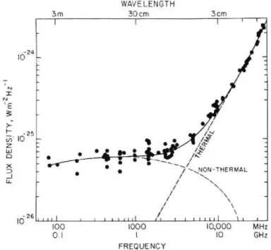
1,1 - _ • • • _ - • w v- - X _ • • • • • /---,NON-THERMAL _ -Lt_ _J/ -26 I I iii.1 it I I 111111 10 ' 100 1000 10 ,000 MHz 01 1 10 GHz FREQUENCY

Fig. 7. Typical radio spectrum of Jupiter from 70 MHz to 30 GHz (black points and solid line). The spectrum in this frequency range consists of non-thermal

(synchrotron) component, which is shown by dashed line and thermal component,

which is shown by dashed line (Carr et al., 1983).

2.2 Spectrum

The observed average spectrum of JSR is shown in Fig. 7 (the dashed line). The

dashed red line in the Fig. is the thermal emission from Jovian disk, which is described

by Planck's radiation law with temperature of 135 K.

According to Equation (32), it is clear that the spectrum of JSR strongly reflects the

electron energy spectrum of the Jovian radiation belt. de Pater and Goertz (1990)

calculated JSR spectrum as a function of L-value assuming the energy spectrum of

relativistic electrons, and compared it to the Pioneer in-situ data at L = 6. They found

that the energy spectrum of relativistic electrons is hardened between L =3 and 1.5,

which may be caused by physical process like a degradation of energy by ring particles

around Jupiter.

de Pater et at. (2003) carried out a brief campaign in September 1998 using 11

antennas in order to determine the spectra of JSR from 74 MHz up to 8 GHz. Comparing

the spectra with that of July 1994 (just before the impacts of Comet Shoemaker-Levy 9),

a significant difference was found (Fig. 8, see page 78). They pointed out as a cause of

the difference that pitch angle scattering, coulomb scattering and/or energy degradation

10 _{TAKUO WATANABE et al .} (a) (b) rotation axis /22 ag_,. .

lir

e940';

oeticP1

i- #

---b

ek-1111/111a4

LH

elliptical>

likAll '14 4_,6 dipole axis

4ei,.

''''oti. ec,

Fig. 9. Directivity of radiated power (a) and polarization (b) of JSR. Those

ters vary with the Jovian rotation, which is called beaming effect (adapted from

Carr et al., 1983).

2.3

Beaming curve

Because the synchrotron radiation has a strong directivity with respect to power and

polarization, an observed JSR shows dependence on the Jovian rotation, which is called

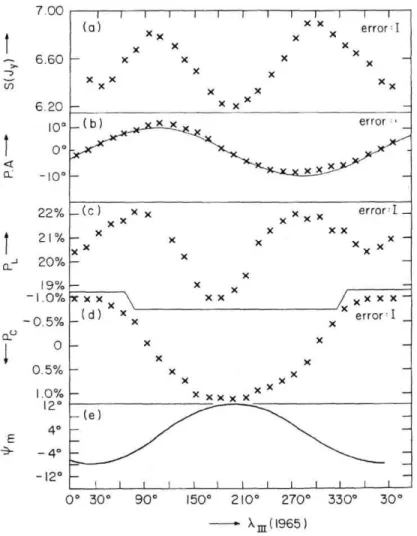
`Beaming curve' (Fig

_{. 9). Fig. 10 shows variations of total power, position angle (angle}

of polarization plain against rotation axis), degree of linear polarization, degree of

circular polarization, and magnetic latitude as a function of System III longitude (de

Pater, 1980).

As the beaming curve has a periodicity as a function of CML, it is possible to expand

to Fourier series, i.e.,

E Aicosti(Acmi,+

Az)]

(34)

1 = 0 , 1,2,• •

where Ai and Ai are the amplitude and phase concerning to period of i times, i.e., Ao

means average intensity over the Jovian rotation. For example in the case of the total

power S, the component of A2 is superior, because it has two peaks at the Jovian equator aligned to an observer.

Because synchrotron radiation has a directivity perpendicular _{to the magnetic field ,}

beaming curve is very sensitive to the direction of the Jovian magnetic field and

declination of the Earth (DE). Dulk et al. (1999a, b) evaluated the Jovian magnetic field

model using beaming curve, in which they used the 3D imaging data of JSR to exclude the effect of line of sight.

2.4 Spatial distribution

The apparent radius of Jupiter is about 25 arc second at opposition. _{Then , an}

antenna with diameter of nearly 80 km is required to resolve the spatial distribution of

0.1 R., at 327 MHz due to the diffraction limit, which is calculated from A/D, where D is

a diameter of antenna and A is wavelength. An interferometer whose diffraction limit

is calculated from Al Ds, where Ds is the separation of antennas, can achieve the spatial

inter-7.00 1 1 i 1 i 1 1 1 1 1 i I I (a) x x error:I

•xx

xx

x x

x x -6.60 -x x x x- -, x X XX x x xX x 6.20- x xx _ 10° - (b) • x x error .

-I

0°-

-

x . cL -10° -x x .. 1 22% - (c ) x xx x x xXXx x x error.I _

1 21%-xx

x

x

xx

x

x-

x x - (2 20% - x 19% - xx -

- 1

_{. 0 %x-x}

_{x x \}

_{x x}

_{4x x x x -}

- a 5% - ( d ) xx x error.I _ u a_

i

0 -

xx

x X - 0.5%- x x x x 1.0%- xxxxxxx - 12° - (e) - E 4°-_ - --- _{- 4° - -} _ -

-12° -

-

I I 1[

I t

I I i I I

i-

0° 30°

90°

150° 210°

270°

330°

30°

---^ X

ja (1965

)

Fig. 10. Beaming

curve (geometrical

variations of parameters) of JSR as a function

of central meridian longitude

(A111)

for total flux (S), angle of polarization plain

against rotation axis (P.A.), degree of linear polarization

(PL),

degree of circular

polarization

(Pc), and magnetic latitude (Om)

(de Pater, 1980).

ferometer system for various frequency and Ds are shown in Fig. 11.

Radhakrishnan and Roberts (1960) and Morris and Berge (1962) resolved JSR source

for the first time using an interferometer.

They used two 90 feet (27 m) antennas at 960

MHz and 1.4 GHz and reported that the source region of JSR extended within 1 (polar

direction) and 3 (equatorial direction) planetary diameters by using the Gaussian fitting

for the observed data.

Berge (1966) first produced a source map (two-dimensional brightness distribution)

by combining the data observed at Owens Valley Radio Observatory (Fig. 12). The

result was almost consistent with the recent observation.

He assumed that the

bright-ness distribution was azimuthally symmetric with respect to the dipole magnetic axis

which tilted about 10° against the spin axis, and fitted Gaussian functions to the observed

12 TAKUO WATANABE et al . 10 :: ::: • : :: ::::::: 3 : : : :::: ::::: W = , 1R3(40

.

11

.4

•

: . : .. ... • ' .. ... ' ' " _{... : • • .. .} arcsec) • u. 01 -rrr7r7FC.7,7•77,77t,,:77^:•:^rp 7777. ... . .. . ... . . ... .. • . : . 0.006. 1 100 .1000 10000 100000 separation[m]

Fig. 11. Diffraction limits (AID) for various frequencies, where D is a diameter of antenna for a single antenna or separation of antennas for an interferometer.

" 1 .... 104 cm-,; ,•20. ... Contour Interval -20.K - • _{.411. A} rusi^ , 20.1( :5•K?

111144:'\

1.

„.

11111111111111111111r

- , TD • 260.1e ... 1.0 0'0 10 210 Fig. 12, Two-dimensional brightness distribution of JSR at CML=20` at a wave

length of 10.4 cm. The spatial scales are in minutes of arc (Berge, 1966).

visibility functions.

Gulkis (1970) obtained one-dimensional equatorial brightness distribution using lunar

occultation on October 19, 1968. The acquired distributions along the equator showed a

clear double-peaked structure with a slight asymmetry and rather extended to far from

Jupiter in lower frequency.

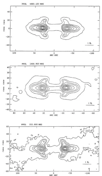
The Very Large Array (VLA) built in 1981 at New Mexico, USA has made a great

improvement on imaging observation of JSR compared with observations in 1970s (e.g.

de Pater, 1980 ; de Pater, 1981). VLA consists of 27 antennas with each diameter of 25 m,

which are mounted on the "Y" formed rail with the farthest distance of 21 km long. Fig.

13 shows a two-dimensional brightness distribution obtained by VLA (de Pater, 1991).

The Australia Telescope Compact Array (ATCA) is another facility that can obtain

two-dimensional brightness distribution of JSR, which consists of 6 antennas with 22 m

diameter each, located along east-west baseline whose span range from 153 m to 6 km.

Leblanc et al. (1997) and Dulk et al. (1997) produced the first three-dimensional

bright-ness distribution of JSR from two-dimensional brightness distributions observed with

PPOL 4885.100 MHZ I I I I • 1 - 40 — — A 20— C)— R C s

E0 —lip'ICI--1

—

C -20 —o 0 _— 1 It, -40 — _— 1 I I [ .I 100 50 0 -50 -100 ARC SEC PPOL 1464.900 MHZ

40

— I

I

I

1

1

1

i

I

d —

30 — — 20 — A C> R c 10-- — So

E0 —

0

0

—

0-10

—

—

-20

—C7

_,

_—

-30—1 R, -40— I I _ I I I I I I I 80 60 40 20 0 -20 -40 -60 -80 ARC SEC PPOL 333.000 MHZ 60 1 I I I 40— o

_{Q - °,1}

El20y 6r

o

7

C. 0

•n4. --0

e.

112)

C. 0. -20 c0 o — 7 o ^ a 0 o °R ,:) I; -40— — 60oo °drio0• 0 !I 1 1 1 I - 100 50 0 -50 -100 ARC SEC

Fig. 13. Two-dimensional brightness distributions obtained by VLA at 6 cm (top), 21 cm (middle), 90 cm (bottom). The maps show only a linealy polarized flux

density (de Pater, 1991).

14 TAKUO WATANABE et al.

4 ,

, .

Fig. 14. Three-dimensional brightness distributions of JSR at 13 cm obtained by

ATCA using the tomographic technique. The viewing CML values are is 90',

150', 210', 270°, 330' from left to right, top to bottom (Sault et al., 1997).

be obtained when adequate views from the different rotational aspects are taken and the

optical thickness of the emission is assumed to be thin. Sault at al. (1997) showed that

a visibility, which is a function of projected baseline vector (V (u, v, w)) and a

three-dimensional brightness distribution (10(x, y, z)) at normalized distance (R0), form a

Fourier pair ; i.e.,

V(u,

v,

w)—()3

fro(x,

y,

z)exp(21.71-(xu+Ryv+

_Acbcdydz,

zw))

₍₃₅₎

where R is distance to source, and A is wavelength. Fig. 14 shows examples of

three-dimensional brightness distribution of JSR observed with ATCA (Sault et al., 1997).

In a three-dimensional brightness distribution of JSR, it is considered that the flux

peak is in the magnetic equator, because under the following reasons ; (1) most electrons

have pitch angle near 90' (2) most intense radiation is almost perpendicular to the

magnetic equator. Using this relation, Dulk et al. (1999a) evaluated the H4 and VIP 4

magnetic field models (Connerney et al., 1998), and Dulk et al. (1999b) showed that

changes of two-dimensional brightness distribution between different declination angles

of the Earth (DE) can be explained by warping of the magnetic equator originating from higher order terms of the intrinsic magnetic field.

de Pater et al. (1997) showed influences of the Jovian ring and inner moon on particle

distribution by comparing models with high-resolution radio images obtained by VLA

(Fig. 15, see page 78). The best-fit model among 16 models is shown in Fig. 16. From

the model, it is confirmed that electron pitch angle distribution becomes isotropic at

Amalthea's orbit around 2.5R, (Fig. 16(b)), which makes 'shoulder' structure (flattening in

intensity curve) in East-West cross section (Fig. 16(d)), and that 80%-100% of electrons

are absorbed by the ring around 1.7R, (Fig. 16(a)), which makes discrete peaks at high latitude in the radio map (Fig. 16(c)).

Bolton et al. (2001) produced a radio map of JSR based on the Divine Garret model (Divine and Garret, 1983) of the electron distribution, and compared with observed radio

maps made with the VLA data. They suggested that the Divine-Garret model

significantly underestimates the number of relativistic electrons( > 1 Mev) as a factor of

iiii,TiiiiiimiiiiIii, 1[1111111 10—(a) ao-(c) - - 40- 3 — — . L.',- 20 —C, -

0rh9

C---

Nx 0411W71 _,)) II 1 —-:M w .-1- - 'ZI --, - -2D — — .3 — model 8 — 40 - - - 40 1 miiiiiiiiipiiiiiiiiii 111111111

0 2 4 6 8 10 12 -BO 40 -40 -20 PIX0 20 ELS 40 60 60

distance in L 1.0 1 1 i 1 1 1 1 I ; 1 1 i I I Iri 100 _ 1 1 i I i 1 1 1 1 1 1 111 1 i i_ 1 (b) _{outside Arrialthea (L=2 .7) - - (d) -} - - 8 inside Amalthea (L=2.4) — 80 — —

-

inside

ring

(L=1

.6)

- I

-

-

- --' - —6 _{/ .' — •••.., 60— —} i -,.-,- - N/ Da- /.--- r- t4/i 4 _—40—i

/

/

, 2---,, — 20— — - .-.'" — _ / - _{._.- -•-' ,} .„

0

₀

1 .1'/1I

₂₀

IAii-i 1 i-i-71

₄₀

₆₀

i I 1

₈₀

o_ILIIImiiiil

₄

₂

₀

_-2

!II

_-4

equatorial

pitch

angle

Jovian

distance

(R,)

Fig. 16. Best-fit model to the VLA observation. (a) Electron flux at the magnetic

equator

(E-20 MeV), (b) pitch angle distribution, (c) modeled intensity

tion, and (d) cross section of modeled intensity distribution along the magnetic

equator (de Pater et al., 1997).

(concentrating to the magnetic equator) than the Divine-Garret model to account for the

observed radio maps. Furthermore, Levin et al. (2001) constructed a model of the

electron distribution to account for the observed radio maps, in which the electron

density was assumed to have a following form

ne(a, L, B)— ALsinnl(ae,)+BLsinn2(ae,),

(36)

where aeq is equatorial pitch angle, parameters of AL, BL, nl, n2 are functions of L,

which are determined from the observed radio maps. Produced JSR maps using the

model showed a good agreement with the observed radio maps and beaming curve .

Recently an attempt to search the fine structure in JSR was performed using Very

Long Baseline Interferometer (VLBI) in 2001 (Kondo, private communication).

2.5

Time variation

While the 'Beaming curve' originates from the viewing geometry between Jupiter

and the Earth as described in Section 2.3, variations which are thought to be originated

16 _{TAKUO WATANABE et al.}

from time variations of the Jovian radiation belt itself have been disclosed in recent

years. The time variation can be roughly classified into three categories ; (1) long term

variation having time scale of decade (top panel in Fig. 17, see page 79), (2) short term

variation having time scale of days or weeks (bottom panel in Fig. 17), and, while peculiar

case, (3) time variation at the time of the impacts of comet Shoemaker-Levy 9 (on July,

1994 in Fig. 17).

2.5.1 Long term variation

Since 1971, the antennas of the NASA Deep Space Network (DSN) have been used

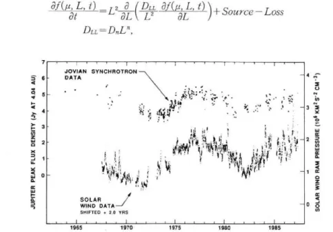
to measure JSR flux density several times in a month, which is known as 'Jupiter patrol'. Bolton et al. (1989) analyzed time serial data from 1963 to 1985 (for about two solar cycles), which include both the 'Jupiter patrol' data and before 'Jupiter patrol' data, and

showed that JSR flux density had a correlation with solar wind parameters (the data

prior to 1974 had been already reported by Klein (1976)). Fig. 18 shows a time variation of JSR flux density and solar wind ram pressure shifted forward 2.0 years, which has the

highest correlation coefficient of 0.87 with 2.0 years lag. From the figure, it has been

believed that solar wind controls the flux density of JSR.

de Pater and Goertz (1994) explained the correlation by means of a simulation.

They assumed that the primary mode of the electron transport is the radial diffusion

driven by the neutral winds in Jupiter's upper atmosphere/ionosphere, and that the

diffusion coefficient is proportion to L3 based on the discussion by Brice and McDonough

(1973). In these assumptions, the phase space density f(p, L, t) is written by the

Fokker-Planck type diffusion equation, i.e.

L, t)

_ataLL2dL

= L2

0 CDLL

of

(AL,L,

t))

_{+ Source—Loss (37)}

DLL= DnLn ,(38) JOVIAN SYNCHROTRON — 3 6 - DATA 4 A 1.• •it • s • , 4 r ; a r-- 3 _{i! •} q;i2(7, 2 -

6011114,1*,

;

LI

• " 3

_tr.

-

₁

.,•4

ITV

i-1 w 0—'•70,04, a. cc SOLAR 4 WIND DATA — 0 51 SHIFTED 2.0 YRS 1965 1970 1975 1980 1985

Fig. 18. Time variation of JSR (top and left axis) and solar wind ram pressure shifted 2.0 years (bottom and right axis). Clear correlation was shown (Bolton, 1989).

where DLL and D,, are diffusion coefficient and diffusion constant concerning L5 (n=3 is

adopted after Brice and McDonough, 1973). Source indicates an injection of particles at

the outer boundary, and Loss includes synchrotron loss formed by Birmingham et al .

(1974), and loss by dust, coulomb scattering, and pitch angle scattering as a function of

L-value.

They assumed that the time variation is not caused by the change of DLL

but by the

change of outer boundary condition, because the change of DLL will cause the change of

radiation peak position, which had not been observed (de Pater and Goertz, 1990). In

this calculation, the outer boundary was set to be L1=50, which did not make significant

differences in the case of L1=20-50, and the time-dependent phase space density at the

boundary was given in proportion to square root of the solar wind ram pressure ,

f L-LicciNs..v's.,(39)

where Ns. and vsw are the number density and velocity of solar wind , respectively.

They, then, searched the best-fit D3 which reproduce observed time variations of JSR.

The assumption of Equation (39) was empirical, but it might be explained if the electron

energy spectrum is power law with-1 because the ratio of energy to magnetic field

strength (first invariant) is constant and the magnetic field strength at plasma pause is

proportional to square root of solar wind ram pressure.

The result is shown in Fig. 19, in which the calculated time variation of JSR agrees

with the observation very well. From the x2 test, D3 was obtained to be 1.3

± 0.2

x

10' s' which was consistent with the observed lag time of 2 year. They also pointed

Do= 1.72E--9- D.--.1.15E-9 -synchrotron —•: radiation -17' -- - D..7 66E-10 - 5 — ,, -., .• _{' ,.!% •• / .."---} .'• _{.— ,.} .!` . '''',. ,A. V ':. ,':',, : ' \ ' • . , '' - 4 .. :•"--, ,,, • '... • • - , _{l 'f} .' / ' :* ‘‘., \ ,'•-• ,'-' ." 2 _{-;', - ' ‘; . ,r•••••:,,' .' :\ •• ..4:., .- . . \ w} Z'. _{z 4 —} - . ,. '....,, dil. .1/ • \ '7 / . :' _• i r t. _. • —' E .1. - - - ._•!;. . ;• : - c4 ,f, t : .. , 3 V -

4i::.`it:,i,I,_

;:,;i.: ''d3js-c,— V . :! !I ..,. ;- j - .' ,q .,•..4; ! '-1

0_j.loq,:t.:::,

7..r"q1

'k;:14i,

_';;

_{IM;'!;'Is110.!}

.--2--2-

laV,i-,:';";,

i

;,:i0'l.t'1'IVA,01

_{..,it;.1 \ ‘}

.;i',1;,;,

2

— ft.t-.J:,,;;-,:

_{$ ' ,1 ,}

_{! ! :,Ir}

1fr-1.—

,-_____

, :,. , :;, ' •

!'

i

' ';f:-:

;i,

; i.,

-

7

I :!!;1

i

,iA !

t1 4:

id— q *!it

' AlH !

_

. ' ' e ' 61 - 1

1 - i-c .v4 _{solar wind ram pressure =}

- d i ^ i i i L , , , , 1 i ! i i I, i . , 1, i 1965 1970 1975 1980 1985 time in years

Fig. 19. Calculated time variation of JSR (solid, dot, and dashed lines). The others are the same as Fig. 18 but solar wind ram pressure is not shifted (de Pater and

Goertz, 1994).

18 TAKUO WATANABE et al.

out that the short term (days-weeks) time variation in JSR could not be explained by the radial diffusion.

2.5.2 Events on the impacts of comet Shoemaker-Levy 9

Shoemaker-Levy 9 (hereafter referred as SL9) was a comet consisting of over 20

nuclei aligned as string, which impacted into Jupiter during the period from July 17, 1994

to July 22, 1994. Because SL9 was crushed into nuclei by the Jovian tidal force at

previous closest approach in 1992, SL9 had dust clouds and larger materials, which were

thought to be injected into the Jovian magnetosphere having influence on not only the

Jovian atmosphere but also environment of the inner magnetosphere.

Prior to the impacts, de Pater (1994) estimated influence of dust on JSR using

numerical simulation, which accounted for the increasing of dust by the same way as de

Pater and Goertz (1990). It was predicted by the simulation that the total power of JSR

would be reduced more than 10% by means of the absorption of relativistic electron by

the dust, and that the spectra of JSR would become hard, and the influence of SL9 would continue for many months.

L , ii. i, ^ , ^ f 1 i m 1 2 4.5 -- 6 cm

_1•

_{Effelsberg..:11}

_{to 13 cmi:•}

_DSN

•- .5 _{.5• Effelsberg ..:}

• •

_-

_{it• •P}

_„,.n

AT

4.0'1. --•• • 7 -5.0 • . . 3.5 '-- .• .•

il

-4- ,5 • •. • _II .,a. _.4.

3.0

1.f.

i1 , , i 1 , , , i I- 4.0 150 200 250 300 150 200 250 300 6.5 _,.,, 'I" _{' ' ' 1 ' , ' ' I _ 7.0 _} = 18 cm • NRL - 21 cm r' ° . Green Bank _

_{< 6.0 - I ••Nancay} -6 _{.5 5- =_ -OA. Parkes}

-

g

=_,Ir‘o•.

_d

0

DRAO

...A Nancay

- P.

5.51 15 T .6.0

if • t. AT __,

Z..).

5.0

.__ {7

_{-: 5.5 X ift}

₄₁

_{. m}

_ •m''' ' - • • • , i 4.5- 1111111111IIL111- _{5 .0 1} 150 200 250 300 150 200 250 300

8 Illlit

_{I 111i1111 _7.5._11TF117111.17i1TI}

_ _ 36 cm • MOST : 70 to 90 cm , o VLA _.-7. 0• DRAO 7-

;

- 6.5

7

=

I i

•

WSRT

:

-

i

11 ! i

7_,,

tiT

I i

- 6 0 -

I

_i_l

- .

't

ii

: f f iiii

I ; I 1 5 , , ^ t il , , i , I m ^ i 50 : , +- . 150 200 250 300 150 200 250 300 Day of 1994 Day of 1994

Fig. 20. JSR flux variation during the SL9 impacts (between dashed line) for various frequencies. Flux intensifications are found for all frequencies, but time scale of flux decay is longer in the higher frequency (de Pater et al., 1995).

The period before, during, and after the collision, intensive observation was carried

out using 11 antennas in the world. The assemble of observations of total flux in various

frequencies is shown in Fig. 20 (de Pater et al., 1995). The total flux increased in all

frequencies against the prediction, but the time constant of dumping of flux was

compa-rable to the prediction. The hardening of the spectrum (de Pater et al., 1995), change of

beaming curve (Bolton et al., 1995), and the brightening of certain location corresponding

to the impacts of large cores (Sault et al., 1997) were also observed. Moreover from the

high-resolution image by VLA, inward shift (toward the planet) of the peak and, the

decrease of the brightness at the instant of the first impact, delay of brightening between

equational peak and high latitude peak, the shift of high latitude peak toward the equator

were observed (de Pater and Brecht, 2001a).

As mentioned above, the drastic change was occurred during the SL9 impacts.

However explanations for all observation results, even increasing of flux density, are not

agreed at all. The complex of following three mechanisms is thought to be possible

(Brecht et al., 2001b) ; sudden increase of the radial diffusion by the electromagnetic

turbulence (de Pater and Brecht, 2001b), acceleration by the collisionless shock in the

same manner as in the interplanetary shock (Brechet et al., 1995), and pitch angle

scattering due to the wave-particle interaction with whistler mode waves (Bolton and

Thorne, 1995).

2.5.3 Short-term variation

The short-term variations having time-scale of few days or weeks had been

report-ed in early 1960's. However those most reports were not confirmed because of

back-ground confusion effects and/or instrumental instabilities (Carr et al., 1983). The

former originates from structure of radio galaxy behind Jupiter, the later is due, for

example, to the variation of the power supply and to ambient temperature fluctuations.

In particular, gain fluctuations can not be distinguished from signal power variations of

a radio star (Kraus, 1986).

Gerard (1970a, b) reported the time variation of JSR quantitatively for the first time,

and suggested the correlation with solar F10.7 variation using the Nancay radio telescope

at 2695 MHz during the period from December 1967 to August 1968. Gerard (1976) also

reported two bursts (probably four), especially the greatest one was enhancement of flux

density of 9% (9 times of rms error), and continued for about a week. Klein, however,

reported that there was no short-term time variation using NASA Deep Space

Instru-mentation Facility at Goldstone at 2388 MHz (12.6 cm) between May and October, 1971

(Klein et al., 1972).

Recent observations have been revealing the feature of short-term time variations

of JSR. The observations based on precise calibrations enable to detect the natural

variation of JSR.

Miyoshi et al. (1999) reported the short-term variation of JSR using the 34 m radio

telescope of Kashima Space Research Center at 2.2 GHz between November 12 to 24,

20 TAKUO WATANABE et al. 1996 November KSRC 34m observation 4.5 „ , ,

(a) derror

Nr 4- • • • • • • - 2;3.5 ••- November, 1996 10 15 20 25 0.4- " " ' ' " ' " 0 2 - - (b) 2 -0.2= -0 4 - Jupiter R A. (J2000) 19h 02' 19h 06m 19h 10"1 19h 14' Jupiter Dec. (J2000) - 22° 55' - 22° 49' - 22° 43' - 22° 36' Fig. 21. (a) Daily variation of JSR at 2.2 GHz observed at Kashima Space Research

Center. Increase of about 14% is clearly shown, which is significantly larger than

error bar (f a). (b) Background confusion level for the sky behind Jupiter

measured 11 month later (Miyoshi at al., 1999).

density was measured using calibration sources of 3C286, 3C295, 3C48, and 3C309.1, and

evaluating the pointing error, extinction by terrestrial atmosphere, gain fluctuation,

distance between Jupiter and Earth, thermal radiation, beaming curve, and background

structure behind Jupiter (shown in Fig. 21(b)).

Because the detected variation had a correlation with solar F10.7 with a 9 day shift,

which corresponds to azimuthal difference between Jupiter and Earth with respect to the

solar rotation, they assumed the variation originated from activation of radial diffusion

induced by UV/EUV heating of Jupiter's upper atmosphere. This idea was originally

predicted by Brice and McDonough (1973). They also performed the numerical

simula-tion which reproduced the observed flux enhancement by increasing 2.5 times of radial

diffusion coefficient (DLL) during 5 days (Fig. 22).

During the encounter of the Cassini spacecraft with Jupiter, the 'Jupiter patrol' was

intensified and JSR observation was made. Then, the existence of short-term variation

was confirmed (Fig. 17(b)).

Gelopeau and Gerard (2001) monitored JSR at 21.3, 18.0, and 9.1 cm from April 1994

to June 1999 using the Nangay Radio telescope. The data clearly revealed the presence

of time variation with the time scale of months and year (Fig. 23), and they call these

`medium -term' variation . Moreover, they reported that spectral index of JSR was

strongly correlated with the 9.1 cm flux density, and time variation was correlated with

almost all solar wind parameters with a lag time of 245 days but dynamic and ion

thermal pressure showed a correlation with a lag time of 615 day.

The existence of short-term variation has been revealed, while the mechanism of

short-term variation is not clarified yet. This is because there are few continuous data

having time resolution of few days because of lack of machine time to observe JSR . So,

0 observed DIM flux

—LS— simulated flux 4.5 5 (a)

0 4'

FE-

0 \

0

re, 01 ' o -.:1 3.5 ,•. t ',..---^ simulation result flux enhancement o 3

ti?.. 3(b)

D„. 3.0 x

i 10-9L3

RJ2/sec

g 2

I. z 1 wg DLL enh?ncement E ° 10 15 20 25 November, 1996

Fig. 22. (a) Comparison of model simulation (line with triangle) with observation (open circle). (b) Time variation of radial diffusion coefficient (DLL) used in the

simulation (Miyoshi et at., 1999).

7-

IIIIIIIIIIIIIIIIIIIIII

1410 MHz

-

6

ii % L S .

IIIIIIIIIIIIIIIIIIE

-- - -I, 5 ,,

I

ila i

;

1

MOM

.cj •<t t.1666 MHz

6

_{4.: • j}

MIN

_{. : •}

_{I ±1a}

8 5 --1---- 3. — hi . C • -1- 11-i- - .,st T.4i 2b _--,,,t4.- ---• 1] 3

_''''

7

IIIIIIIIIIIIIIIIIIIIIIIIIIIIIIIIIIIIIIIIIIIIIIIIIIIIIIIIIIIIIIIII

3" MHz

a)

M.

x 6

=

.f

p,_

.. :

1±1cr

ME

LL 5 4'- '`. '--t

- - It:

1

1 —

'-. - L - - - --: -1.-

MEE

' MEM

_.

,-. II' • .•

1 111111111111111111111111111111111111111111111111

4

Mr

1994 1995 1996 1997 1998 1999

_{Fig. 23. Flux densities of JSR at 1410 MHz (top), 1666 MHz (middle), and 13300 MHz}

(bottom), and typical error bar. Dashed line is a references level before the SL9

impacts and start point of gray-shaded line represents the minimum value of flux

defined as 3% of histogram of flux (Gelopeau and Gerard, 2001).

characteristics of the short-term _{variation and the physical processes .}

3 Remote sensing of the Jovian magnetosphere

3.1 Summary of in-situ observation of the Jovian radiation belt

Until now, 7 spacecrafts visited Jupiter as listed in Table 1.

The orbits of the spacecrafts projected onto the magnetic meridian plain are shown

22 TAKUO WATANABE et al.

Table 1. The spacecraft visited Jupiter.

Closest approach type

Pioneer 10 Dec., 1973 fly-by

Pioneer 11 Dec., 1974 fly-by

Voyager 1 Mar.,1979 fly-by

Voyager 2 Jul., 1979 fly-by

Ulysses Feb., 1992 fly-by

Galileo Dec., 1995-Sep.,2003 satellite

Cassini Dec., 2000 fly-by

Pioneer 10, 11, and Galileo probe. The orbits of other spacecrafts were designed to

avoid radiation damage.

The features of the Jovian radiation belt observed by the spacecrafts are discussed

in the following section.

Flux distribution of the Jovian radiation belt

Fig. 25 shows the contour of iso-counting rate of omni-directional electron with E>

21 MeV, which represents the structure of the radiation belt (Van Allen, 1974). The

contour is extrapolated from the observed points along the Pioneer 10 and 11 paths

assuming that the structure is uniform for the dipole magnetic field. There is no slot

region which divides the inner and outer radiation belts as can be seen on the earth. The cross section of Fig. 25 at the magnetic equator is shown in Fig. 26 (Van Allen,

1976). The inner edge of the radiation belt measured by Galileo probe was 1.35 Rj for all

5 R J 4- zx103 PIONEER 10 { 11 3 - 2 - t0005 .104 1

0 4

.---3--''.''))""°6

17))

-2 - -3 - -4 - - _5 0 1 2 3 4 5 6 7 8 9 10 1 1 12 13 14 15 RJ Fig. 25. Iso-counting rate contour of omni-directional electrons with E>21 MeV,

which represents the structure of the radiation belt (Van Allen, 1976).

1 rI ! I I I I I

EQUATORIAL OMNIDIRECTIONAL

INTENSITY — ELECTRONS Es> 21 MeV

7 PIONEERS 10 AND II 10 : 1 • L _{..1•3.45x108 expf—r/1.42)} FOR 3.5 r s 12 Rj icg M 0.16- s10 - 105 • 104 0 2 4 6 8 10 12 141:14 RADIAL DISTANCE

Fig. 26. Cross section of Fig. 25 along the magnetic equator (Van Allen, 1976).

particle species (Fischer et al., 1996). Energy spectrum of the Jovian radiation belt

The energy spectrum at various L-values is shown in Fig. 27 (Baker and Van Allen,

1976). The hardening of energy spectrum as the L-values decreases represents the

existence of some strong acceleration mechanism in the inner magnetosphere.

Time variation of hot electron

Galileo spacecraft observed some time-variations of energetic particles with

energies of several hundreds keV, which are injected from the outer magnetosphere and

become possible to be detected at the satellite orbit around Jupiter. For example,

dynamic injection and dispersion of the energetic particles at L=11 (Mauk et al., 1997)

and longitudinally confined charged particle injection like substorm on the Earth (Mauk

et al., 1999) are reported and argued in the relation with the dynamics of the Jovian

magnetosphere.

In-situ observation of JSR

The in-situ observation of Jovian synchrotron radiation was carried out by

repeat-ing raster scans of Cassini primary communication antenna from the distance of 149 R,

by Bolton at al. (2002) (Fig. 28, see page 80). The observed frequency was 13.8 GHz,

which corresponds to the concerning electron energy of 50 MeV as can be obtained from

Equation (28). The existence of these ultra relativistic electrons with higher energies

24 TAKUO WATANABE _{et al .} 109 2. 2 INBOUND ::OUTBOUND-- _{_} , , PASS -PASS • . . 108 .. , . . .. . , (i.,.N.,,^-1111111111: _ - m-. ''' , . _. u., 10 F ,, . E.- , \ , Z 7. \ \ . 0 - \ \ \ - , - CC - \ \ F .-- - \ 11 (..) ., \ \ . • : LLJ - \ _• \ • 10 ‘ 1.1.,-'1 7 . ET ^ 1 : % \ i— - ^ - \ _ (7)_A- z,.1\- ^ W S \ ‘ - \ z 10F7 — \-:• \ 1 2 : - 0- \ " IX _- . I— 1 1 _ C_{.) -} 41 Lai 4 spEcTRAL SPECT RAL1 W102-PARAMETERSPARAMETERS7: SYMBOL R j Lnl,7: : SYMBOLlijL 11,n 4 W-1 i_ : • 20 21.1 2,5,2.S- _, • 3 3.2 72.4 1m • 0)- _ • 18 20.0 2.0,2.6\1 -

-,_e•:'6:5410305,4.:I::11.°2)/1'C'

-

0-•::11:.0::::::70't:• IT)1"NT

V)

1

3::I:::26°51:c''

I')}EuR

\

al io , • i2 i2.1 iS.6.1 Int • LI) — —- _{1 _.}

<1 a

nI08118.725°0,67.1)1m • 1.31 }Et': : • 12 13.1 9,4.2 • 14 16.2 5,2.8 }GANT a

o :*4.10 I°:13 1:nn :1021' • - } I° 1 - - • le ie.° 2,2.4 ^ 16 16.5 3, 3. 1

_ • 3 3.0 4,2.2 Inn • 01- -1 ^ 20 21.2 8,2.6 11 -

\ 2

102 101 100 101102 102 10-1100 101 102

Fig. 27. Energy spectrum for various L-values for inbound pass (left) and outbound pass (right) of Pioneer 10. The hardening of spectrum as L-value decreases

represents the existence of acceleration (Baker and Van Allen, 1976).

3.2 Necessity of remote sensing of the Jovian radiation belt

In-situ observation of the distribution and its dynamics of the energetic particles has

a fundamental difficulty of separating time variation from special distribution. So many

observation reports treated that there is no time variation with respect to velocity of

spacecraft. the Galileo spacecraft, which became a satellite of Jupiter, can reveal the

time variation separating from special distribution by means of accumulation of a lot of

orbit data around Jupiter. However the detected features are restricted to the vicinity

of the satellite orbit. In particular for the case of Jupiter, it is impossible to measure

relativistic particles by in-situ observations due to the radiation damage by the

relativis-tic parrelativis-ticles themselves. Thus it is important for the study of the Jovian radiation belt

to perform the ground-based remote sensing of the Jovian synchrotron radiation (JSR)

emitted from the relativistic electrons.

In order to discuss the time variation of JSR with the time scale of days to weeks,

a continuous observation is necessary. However it is generally impossible to make

continuous observations by using a common use antenna because of the machine time.

synchrotron radiation.

To develop the observation system by ourselves has also an

importance to establish basic techniques for a future interferometric observation which

can image the 2-dimensional Jovian synchrotron radiation distribution.

Note that the inner radiation belt on the Earth also has a time variation of few days.

Up to 90's the radiation belts on the Earth have been thought to be static and stable.

However, recent in-situ observations have been revealing the dynamical feature of the

radiation belts. The dynamic feature of the inner and outer radiation belts observed by

the CRRES spacecraft is shown in Fig. 29 (see page 80) (Baker et al., 1994).

3.3

Antennas for JSR

3.3.1 Required specifications for the JSR observation

The observation system must have a sufficient sensitivity to detect the time variation

of JSR. Minimum detectable sensitivity of a receiving system is defined by comparing

the levels between the fluctuation of the signal, LiTRMS,

and the amplitude increased from

the average level of a star, ZITstar, (Fig. 30), where T in Kelvin. The signal power is

represented in wattes/Hz as ;

w=kT

(40)

where k is Boltzmann's constant (1.38

x 10' [J/K1). The output power of kT is equal

to the output power of the resistor with the temperature of T and also equal to the

output power of an antenna surrounded by blackbody with the temperature of T.

Fluctuation of signal (JTRMS)

is proportional to the background level (Tsys) and

inversely proportional to 14fr by statistical effect, where 4f and z- are the bandwidth

of the signal and time constant of the signal integration of the receiver, respectively.

The product of 4f and r becomes an single quantity because the signal of bandwidth of

has a correlation with a time of 1/ Zif. So d TRMS can write as

Tsys

4T

Rms= (41)

Increased signal level of the star with flux density of S is described as,

w=SA,(42) Peak-to-peakTm~= AT ( temperature

\I TIT

T (background)IT (background) T (background)

Fig. 30. The basic idea of minimum sensitivity. The minimum sensitivity is mined by comparing JTRms and Tsar (Kraus, 1986).