東北大学機関リポジトリTOUR

(1)

Retrieval of wind velocity in Venusian

nightside mesosphere from CO2 absorption

observed by mid-infrared heterodyne

spectroscopy

著者

Takami Kosuke

学位授与機関

Tohoku University

(2)

Retrieval of wind velocity in Venusian nightside mesosphere from

CO

2

absorption observed

by mid-infrared heterodyne spectroscopy

9

467

(3)

(4)

Doctoral Thesis

Retrieval of wind velocity in Venusian nightside mesosphere from

CO

2

absorption observed

by mid-infrared heterodyne spectroscopy

9

467 v8 23

5 O

Kosuke Takami

x

0

1

0 O 1

C

i

0

1

(5)

(6)

Abstract

This study presents a new attempt to retrieve Doppler wind velocity as well as temperature profile in the Venusian nightside from CO2 absorption spectra resolved by mid-infrared (MIR) heterodyne spectroscopy. The target sensitivity of the Doppler wind velocity retrieval aims to constrain the vertical transition of the wind regime at altitudes below 100 km where the retrograde super-rotational zonal (RSZ) wind changes to the subsolar point to the antisolar point (SS-AS) flow. We aimed to achieve the wind velocity and temperature retrieval requirements with an accuracy better than ±50 m/s and ±15 K. These requirements are based on the following considerations. For the wind velocity retrieval, a numerical model study showed that the transition between the RSZ wind and the SS-AS flow occurred at an altitude of ~90 km (Alexander, 1992). The wind profile in the dawn side was gradually varied from ~50 m/s westward at 80 km to ~50 m/s with eastward direction at 100 km. For observational identification of this transition, the accuracy of the wind velocity retrieval should be better than ±50 m/s. For the temperature retrieval, we considered the VEX SPICAV result which found the warm layer as a reference. This was 30–70 K higher than temperature obtained by previous measurements, and it was interpreted to be caused by the adiabatic heating during the air subsidence of the SS-AS flow (Bertaux et al. 2007; Gérard et al. 2017). For observational identification of such warming, the retrieved temperature accuracy should be better than ±15 K.

A method which was supposed in Nakagawa et al. (2016) was used in this study for retrievals of temperature and wind velocity profiles from CO2 absorption spectra. They showed feasibility of retrieval for Venusian and Martian atmosphere, but do not refer to its verification. Based on the errors originating from uncertainties in a priori profiles, we estimated achievable sensitive altitude and retrieval accuracy using model spectra generated from various temperature and wind profiles with different noise levels. The evaluation suggested that temperature profiles can be retrieved at altitudes of 70 - 95 km range with vertical resolution of 5 km and retrieval accuracy of ±15 K. The assumed nominal noise level was 1.0 erg/s/cm2_/sr/cm-1_{. For data with a higher signal-to-noise ratio} (higher radiance and/or lower noise level), the retrieval accuracy can be improved and the upper boundary can be extended to 100 km. By contrast, the wind velocity profile was more difficult to obtain but still could be retrieved at an altitude of approximately 85 km with a vertical resolution of 10 km. For data with a higher signal-to-noise ratio, the retrieval accuracy became better, changing from ±50 m/s for noise levels of 1.5 erg/s/cm2_/sr/cm-1_{to ±25 m/s for noise levels of 0.5 erg/s/cm}2_/sr/cm-1_{. This result provides}

(7)

the first validation of a method for wind velocity retrieval in the Venusian mesosphere at altitudes of 85 - 95 km.

We applied our retrieval method to Venus MIR spectra obtained by HIPWAC observations in May 2012 with data partially in common with the study by Stangier et al. (2015). We confirmed that our retrieved temperature profiles were in good agreement with the results of Stangier et al. (2015) obtained by different retrieval and also with radio occultation studies at coordinate observed point by Pätzold et al. (2007). The agreements supported validity of our method. Next, we retrieved the wind velocity at the altitudes of 80 - 95 km. The retrieved results at 33˚ S and 3 LT are 35 ± 28 m/s at 84 ± 6 km and 144 ± 70 m/s at the altitude of 94 ± 7 km, corresponding to the SS-AS flows at both altitudes. This result is unexpected because it is in the opposite direction of the RSZ wind. The retrieved results at 67˚ N and 0 LT were 66 ± 73 m/s at 80 ± 7 km and 112 ± 69 m/s at 90 ± 7 km, indicating the potential meridional circulation toward the equator at both altitudes. These velocities were consistent with the wind profile obtained by GCM of Gilli et al. (2017), but the retrieved wind at 33˚S was stronger. Our results suggested that the transition region between the RSZ wind and the SS-AS flow is found lower than 90 km which had been predicted to be the transition altitude.

We conducted observation by our MIR heterodyne instrument MILAHI at the summit of Haleakala" on November 11 - 13, 19, and 20, 2018 targeting wind velocity at the evening terminator in the Venusian mesosphere. Observed points were equator (EQ) at LT of ~22:00 on November 11 - 13, 33˚N at LT of ~23:00 on 19, and 33˚S at LT of ~23:30 on 20. We could retrieve wind velocities from four spectra obtained on November 11, 12, 13, and 20. Retrieval showed wind velocities larger than 65 m/s from EQ11 and 150 m/s from EQ12, EQ13 and 33S20. Although mesospheric wind velocity has been expected to approach smaller than 50 m/s from the RSZ wind between 75 km and 95 km by numerical model of Alexander (1992), this observation suggested that there is much stronger wind velocity larger than 150 m/s. We cannot classify the retrieved wind as the RSZ wind or the SS-AS flow due to same wind direction of the dynamics on the dusk side. There is also the possibility of superposition of two dynamics.

This study established the method of retrieving wind velocity and temperature in the Venusian mesosphere using MIR heterodyne spectroscopy by means of radiative transfer and Levenberg-Marquardt method. The retrieved altitude is the region where wind velocity along line of sight has not been observed by remote sensing so far due to its technical difficulty. Additionally, we studied mesospheric wind on both dawn side and

(8)

dusk side. Retrieved wind velocities were strengthened toward a direction corresponding to the SS-AS flow on both sides. This study could conduct only one observation campaign at each side. We should conduct more MIR heterodyne observations in order to verify dynamics in the mesosphere and investigate temporal and spatial variations. Our advantage is to be able to observe the mesospheric wind continuously by dedicated telescope: Tohoku university 60-cm telescope. The investigations give us important information for comprehensively understanding Venus upper atmospheric structure.

(9)

(10)

.

Acknowledgements

I would like to express my sincere gratitude towards Associate Professor Isao Murata, for his special support and guidance throughout the course of my study. His patient assistance was essential to finish writing my doctoral thesis. I wish to express my deep gratitude to Professor Yasumasa Kasaba for his valuable discussion and continuous help. I am deeply grateful to Assistant Professor Hiromu Nakagawa for his collaboration with my study. The MILAHI used in this study was developed with him. I would like to express my special thanks to Professor Naoki Terada for his supports and encouragement regarding my study I wish to deeply thank Assistant Professor Takeshi Kuroda for his helpful advices.

I would like to express great thanks to Associate Professor Hideo Sagawa for his supports through my study and kindly discussion of various matters.

In my academic life, many staffs of the Tohoku University gave me precious comments about my study. I would like to thank Professor Takahiro Obara, Professor Yuto Kato, Associate Professor Takeshi Sakanoi, Associate Professor Hiroaki Misawa, Associate Professor Fuminori Tsuchiya, Associate Professor Atsushi Kumamoto, Assistant Professor Masato Kagitani, and Assistant Professor Tomoki Kimura.

I am obliged to Mrs. Miyako Tanno for helping my life in laboratory.

I would like to express my appreciation to Dr. Pia Krause for her management of valuable discussion in Cologne, and Dr. Oleg Benderov for his friendly supports and cooperation of experiments in Moscow. I am grateful to all members of University of Cologne and Moscow Institute of Physics and Technology for their kindness and support.

I am indebted to all colleagues of the Planetary Atmosphere Physics Laboratory of Tohoku University.

(11)

(12)

.

List of figures

Figure 1.1 Wind velocity profile derived from thermal wind deduced from pressure gradient obtained by Pioneer Venus orbiter and probes (Fig.27 in Seiff et al., 1980). OIR means the Orbiter Infrared Radiometer. NORTH means North probe at 59.3˚N and local time of 3:35. DAY means day probe at 31.2˚S and local time of 6:46. DLBI means the Large Probe Differential Long Base Line Interferometer.

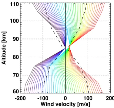
Figure 1.2 Wind profile from the surface to the exobase calculated by numerical model (after Fig.1 in Alexander et al., 1992). The wind profile in the dawn side (8:00 LT) and dusk side (16:00 LT) are shown. Dashed line means the wind is not calculated adequately due to less previous observations to deduce wind velocity.

Figure 1.3 Overview of the RSZ wind and SS-AS flow. The RSZ wind located at an altitude of 70 km flows to westward. The SS-AS flow dominating at the altitudes above 120 km flows from dayside to nightside derived by a temperature gradient.

Figure 1.4 Simulation of the upward radiance for line at a wavenumber of 1053 cm-1_{on Venus.}

Spectra at a number of selected altitudes from 70 to 200 km are shown in left panel. In central panel, radiance profile obtained from the results of the left panel at 2 different wavenumbers: line wing and line core correspond to spectral positions of 0.002 and 0.0035 cm-1_{in the left panel, respectively. Altitude derivatives of the functions in central panel at}

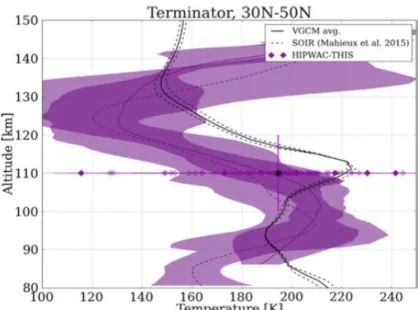
those two wavenumbers are shown in right panel (Fig.8 in López-Valverde et al., 2011). Figure 1.5 Mean profiles of the temperature as function of altitude, predicted by the

LMD-VGCM in the latitudinal range of 30°N–50°N (solid black line) at the terminator, with standard deviation (dashed black line), together with SOIR/VEx temperature retrieval results (purple dashed line for the morning and solid for the evening terminator) at the same latitudes bin. SOIR standard deviations are also represented with shaded purple area (after Mahieux et al., 2015). Temperature results at 110 km from ground-based

observations (Krause et al., 2015) are also shown in purple diamonds (Fig. 11 in Gilli et al., 2017).

(17)

.

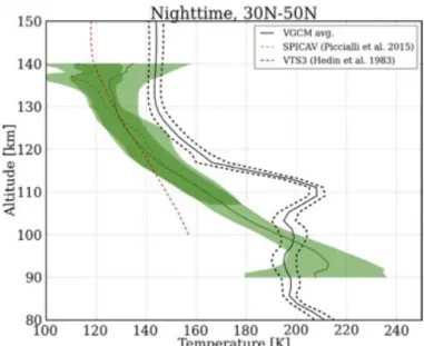
Figure 1.6 Mean profiles of the temperature as function of altitude, predicted by the LMD-VGCM in the latitudinal range of 30°N–50°N (solid black line) at nighttime (19-5 LT), with standard deviation (dashed black line), together with SPICAV/VEX temperature retrieval results (in green): 30°N–50°N (dashed line) and 30°S–50°S (solid line). Standard deviations are also represented with the shaded green area (after Piccialli et al., 2015). The temperature calculated by model by Hedin et al. (1983) at nighttime is also plotted (red dashed line), as reference (Fig. 10 in Gilli et al., 2017).

Figure 2.1 Upper panel shows the transmittance of the atmospheric spectrum of lower side band in blue line and upper side band in green line. The red line corresponds the LO frequency. Middle panel is the image of superposition of lower side band and upper side band. Bottom panel shows the observed spectrum which is the average of spectra in lower side band and upper side band by DSB detection. It is noted that the horizontal axis represents IF.

Figure 2.2 The system noise temperature #$%$ at 7.7 (dotted line) and 10.3 µm (solid line)

from Nakagawa et al. (2016). The averaged values of #$%$ are 3500 and 2500 K at 7.7 and 10.3 µm, respectively. The spectral binning is 4 MHz. It is also noted that the quantum limits of 1869 K at 7.7 µm (dot-dashed line) and 1397 K at 10.3 µm (dashed line).

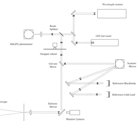
Figure 2.3 Optical configuration of HIPWAC from Stangier (2015)

Figure 2.4 Optical configuration of MILAHI modified from Nakagawa et al. (2016).

Figure 2.5 Image of CCD at beam patterns of MILAHI for apparent Venus. Upper left, upper right, bottom left, and bottom right panels are image of CCD camera seen in beam pattern of obtaining signals of &', (), &), and (', respectively. Right figure shows pointing of telescope for apparent Venus. Solid and dotted squares are image of CCD camera. Red circles are FOVs of heterodyne at MIR. Orange regions are the crescent Venusian dayside, and white region in dotted line is Venusian nightside.

Figure 3.1 Overview of the method of AMATERASU analysis: Blue and green lines are a priori and the best fit of profiles, spectra and residuals, respectively.

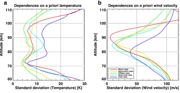
Figure 4.1 Five model spectra as emulated CO2 absorption line profile. Color lines show the

(18)

(semi-. cold case, sky blue), 0 K (VIRAex case, in green), +15 K (semi-warm case, yellow), and +30 K (warm case, red) cases from VIRAex. For all of these, the wind velocity profiles are set to 0 m/s at all altitudes. White noise with the RMS of 1.0 erg/s/cm2_/sr/cm-1_{is added. In}

a, black lines show examples of 13 a priori spectra generated from temperature profiles of -30 - + 30 K from VIRAex with 5 K steps at all altitudes. The wind velocity profiles are 0 m/s at all altitudes. In b, black lines show examples of 5 a priori spectra generated from the wind velocity profiles of -200 - + 200 m/s at 100 m/s steps at all altitudes. The temperature profiles are VIRAex.

Figure 4.2 Retrieved temperature profiles from the model spectrum with the temperature of VIRAex and wind velocity of 0 m/s (green line in Fig. 4.1). Colored lines show the profiles retrieved with 169 a priori temperature profiles (orange: higher temperature, blue: lower temperature) in a. Black line is the original VIRAex profile. Temperature differences between the retrieved profiles and the original profiles in b. Black dashed lines show the standard deviation of the differences with 1 km steps.

Figure 4.3 Retrieved wind velocity profiles from the model spectrum generated from

temperature of VIRAex and wind velocity of 0 m/s (green line in Fig. 4.1). Colored lines show the profiles retrieved with 41 a priori wind velocity profiles (red: positive wind velocity, blue: negative wind velocity). Black dashed line shows the standard deviation for these profiles.

Figure 4.4 Standard deviations of the retrieved temperature in a and wind velocity in b from five model spectra shown in Fig. 4.1. The meaning of the colored lines is the same as that in Fig. 4.1. Green lines (VIRAex case) in a and b are the same as the black dashed lines in Figs. 4.2a and 4.3, respectively.

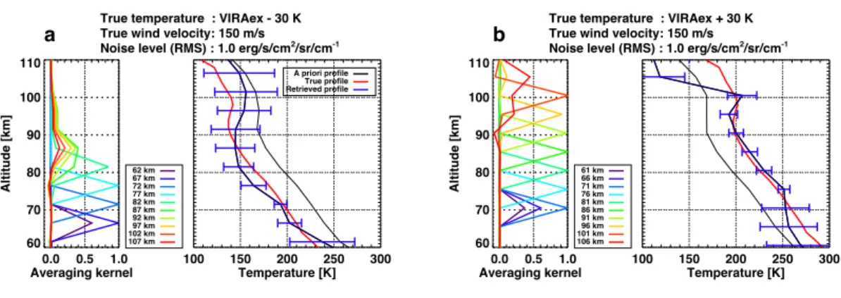
Figure 4.5 Examples of the model spectra synthesized from the temperature profiles of the cold case (VIRAex - 30 K) in a and the warm case (VIRAex + 30 K) in b. Upper panels show the model spectra (blue), a priori spectra (black), and retrieved spectra (red). Lower panels show the residuals between the model and retrieved spectra. Model spectra were generated with the wind velocity profile of +150 m/s at all altitudes, including white noise with the

(19)

.

RMS of 1.0 erg/s/cm2_/sr/cm-1_{. In both, the a priori profiles are VIRAex for the temperature}

and 0 m/s for the wind velocity at all altitudes.

Figure 4.6 Temperature profiles retrieved from the model spectra shown in Fig. 4.5. In the right panels of a and b, blue, red and black lines represent the retrieved, model, and a priori (VIRAex) profiles, respectively. Blue horizontal lines are the retrieval errors calculated using Eq. (4.51). Left panels of a and b show the AKs. The peaks of AKs are the sensitive altitudes, and full-widths at half-maximum are their vertical resolutions.

Figure 4.7 Wind velocity profiles retrieved from the model spectra of the cold case in a (VIRAex -30 K) and the warm case (VIRAex + 30 K) in b. Other symbols are the same as those in Fig. 4.6.

Figure 4.8 Statistical results for a, b retrieved temperatures and c, d wind velocities from the model spectra with 41 wind velocity profiles of -200 to +200 m/s at all altitudes and white noise with the RMS of 1.0 erg/s/cm2_/sr/cm-1_{. The cold case results are shown in a and c,}

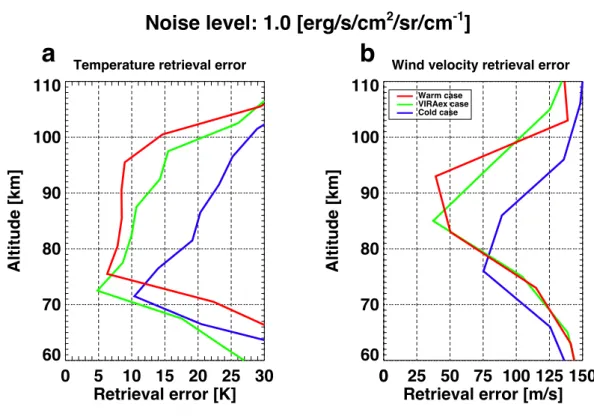
and the warm case results are shown in b and d. In the right panels of a - d, red lines are the mean differences between retrieved and model profiles, gray areas are the standard deviations of the differences, and blue dashed lines are the mean retrieval errors. Left panels a - d show the same AKs in Figs. 4.6a, b, 4.7a, and b, respectively, as examples. Figure 4.9 Mean retrieval errors of the temperature in a and wind velocity profiles in b. Color

lines show the errors in the retrieval from the model spectra in the cold case (blue), VIRAex case (green), and warm case (red), with 41 wind velocity profiles and white noise with the RMS of 1.0 erg/s/cm2_/sr/cm-1_.

Figure 4.10 Model spectra generated from the temperature profile of the VIRAex case and the wind velocity profile of +150 m/s at all altitudes with small noise level (0.5

erg/s/cm2_/sr/cm-1_{RMS) in a and with large noise level (1.5 erg/s/cm}2_/sr/cm-1_{RMS) in b.}

Upper panels show the model spectra (blue) and retrieved spectra (red). A priori spectra (black) are overlapped almost exactly with the red lines and are not seen well. Lower panels show the residuals of retrieved spectra from the model spectra.

(20)

. . Figure 4.11 Temperature profiles retrieved from the model spectra with small noise level (0.5

erg/s/cm2_/sr/cm-1_{RMS) in a and large noise level (1.5 erg/s/cm}2_/sr/cm-1_{RMS) in b shown}

as blue lines in Fig. 10. Other symbols are the same as those in Fig. 4.6.

Figure 4.12 Wind velocity profiles retrieved from the model spectra with small noise level (0.5 erg/s/cm2_/sr/cm-1_{RMS) in a and large noise level (1.5 erg/s/cm}2_/sr/cm-1_{RMS) in b shown}

as blue lines in Fig. 10. Other symbols are the same as those in Fig. 4.7.

Figure 4.13 Mean retrieval errors of the temperature in a and wind velocity profiles in b. Color lines show the errors in the noise levels of 0.5 (red), 1.0 (green), and 1.5 (blue)

erg/s/cm2_/sr/cm-1_{RMS, with the temperature profile of the VIRAex case and 41 wind}

velocity profiles.

Figure 5.1 Observation geometry of Venus during May 2012. Blue cross represents the anti-solar point. Green circles are the observed locations, (left) 33SLT3 (33° S, 3:30 LT) and (top) 67NLT0 (67° N, 00:00 LT). Their sizes are the field of view (0.9 arcsec). The angular diameter of the apparent disc varied between 50.4 arcsec on May 19 (shown in this figure) and 52.5 arcsec on May 22.

Figure 5.2 Observed spectra obtained by HIPWAC on May 19 - 22, 2012 at 33SLT3 in a and 67NLT0 in b. Upper panels in a and b show the observed spectrum (blue), a priori

spectrum (black), and retrieved spectrum (red). Lower panels in a and b show the residuals of the observed spectrum relative to the retrieved spectrum. The noise levels are 0.6 erg/s/cm2_/sr/cm-1_{in a (integration time: 100 minutes on 19 - 20 May) and 1.9}

erg/s/cm2_/sr/cm-1_{in b (integration time: 30 minutes on 22 May). A priori profiles are based}

on VIRAex for the temperature and 0 m/s for the wind velocity at all altitudes.

Figure 5.3 Temperature profiles retrieved from the spectra at 33SLT3 in a and 67NLT0 in b shown in Fig. 5.2. The symbols are the same as those in Fig. 4.6.

Figure 5.4 Retrieved temperature profiles at 33SLT3 in a and 67NLT0 in b. Blue cross lines show the retrieved results with their errors (horizontal) and vertical resolutions (vertical), shown in Fig. 5.3. Green lines show the values in Fig. 7 of Stangier et al. (2015). Red line shows the VeRa results at 33.8˚S and LT 03:49 on 20 May 2012 in a (Stangier, 2015) and

(21)

..

at 71˚N and solar zenith angle of ~100˚ in b (Pätzold et al. 2007), derived with three different upper boundary temperature conditions of 170, 200, and 230 K.

Figure 5.5 Wind velocity profiles retrieved from the spectra at 33SLT3 in a and 67NLT0 in b shown in Fig. 5.2. Other symbols are the same as those in Fig. 4.7.

Figure 5.6 Retrieved wind velocity profiles at 33SLT3 in a and 67NLT0 in b. Blue cross lines show the retrieved results with their errors (horizontal) and vertical resolutions (vertical), shown in Fig. 5.5. Black solid lines are the wind velocity profiles deduced by a GCM study from Gilli et al. (2017). Black dashed lines in a show the model value obtained in Alexander (1992). The zonal and meridional wind velocities are converted to the wind velocities along the line-of-sight of the observing geometries

Figure 6.1 Observation geometry of Venus during Nov. 2018. Green circles are the observed locations, (upper) 33˚N on Nov. 19, (middle) the equator on Nov. 11-13, and (lower) 33˚S on Nov. 20. Their sizes indicate the field of view (4 arcsec) of MILAHI. Brue cross represents the anti-solar point. The angular diameter of the apparent disk varied from 54.8 arcsec on Nov. 11 (shown in this figure) to 47.8 arcsec on Nov. 20.

Figure 6.2 Spectra obtained on Nov. 11-20, 2018. EQ11, EQ12, EQ13, 33N19, and 33S20 are shown in a, b, c, d, and e, respectively. There are several frequency channels with very large noises and they are removed from the plot (masked with gray lines). The removed IF frequencies are shown as red lines in Fig 6.5. The Doppler shifts of CO2 line due to

relative motion of Venus with respect to the observer are 629 MHz, 650 MHz, 689 MHz , 862 MHz, and 868 MHz on Nov. 11, 12, 13, 19, and 20, respectively, and they are

indicated by red lines. The spectra are corrected for the change of the Doppler shift during the data integration.

Figure 6.3 Image of the optical CCD camera at beam patterns of MILAHI in the case of large apparent Venusian diameter. Upper left, upper center, upper right, bottom left, and bottom right panels are the beam patterns of obtaining signals of &', (), *, &), and (', respectively. Bottom right figure shows pointing of telescope for apparent Venus. Solid and dotted squares are the image of CCD camera. Red circles are FOVs of heterodyne at

(22)

.. MIR. Orange regions are the crescent Venusian dayside, and white region in dotted line is Venusian nightside.

Figure 6.4 Gas-cell spectra obtained during each observation date are shown in the upper panels of a, b, c, d, and e. Black lines are C2H4 line at IF of 812 MHz, corresponding to 28358963

MHz and 945.953202 cm-1_{. The number of gas-cell spectra are different between each}

observation date. Color lines represent gas-cell spectra and their gaussian fitting lines. The color represents the timing of data acquisition: bluer and redder ones are obtained earlier and later, respectively, during each observation date. The lower panels of a’, b’, c’, d’, and e’ are enlarged figures of upper panels with the line center of C2H4 (812 MHz) setting as 0

MHz of the abscissa. Line centers of the gas spectra are added as the vertical lines with each color.

Figure 6.5 Spectra obtained on Nov. 11-20, 2018. EQ11, EQ12, EQ13, 33N19, and 33S20 are shown in a, b, c, d, and e, respectively. Blue lines are the spectra after removal of the spiky noises. Red lines are the spiky noises that removed from the data. Green lines are the Gaussian line-shape fitted spectra used for the noise level evaluation.

Figure 6.6 The results of spectra fitted with AMATERASU. EQ11, EQ12, EQ13, 33N19, and 33S20 are shown in the upper panels of a, b, c, d, and e, respectively. Black, blue, and red lines are a priori, observed, and retrieved spectra, respectively. Vertical red and black lines represent IFs of the line centers of the best-fitted (wind retrieved) and a priori (0 m/s wind) spectra, respectively. The line center IFs of the best-fitted and a priori spectra are 615 and 629 MHz at EQ11, 619 and 650 MHz at EQ12, 641 and 689 MHz at EQ13, 872 and 862 MHz at 33N19, and 847 and 868 MHz at 33S20, respectively. Residuals between the observed and best-fitted spectra are shown in the bottom panels of a, b, c, d, and e. RMS of residuals are written above each panel.

Figure 6.7 Enlarged residuals between the observed and best-fitted spectra in Fig. 6.6. Red solid lines are the line centers derived by the Gaussian line shape fitting as shown in Fig.6.6, with showing a range of an averaged full-width at half-maximum (152 MHz). Table gives RMSs of the residuals estimated from full spectra and the data only around the line center within 152 MHz width. For clarity, RMS of the near-line center is colored with

(23)

..

green if it is smaller than the RMS level estimated from full spectrum, and with red for vice versa.

Figure 6.8 Wind velocity profiles retrieved from the spectra of Fig. 6.2. The AK and retrieved wind velocity of EQ11, EQ12, EQ13, and 33S20 are shown in a, b, c, and d, respectively. Black and blue lines in right panel of each figure are a priori and retrieved wind velocity profile, respectively. Horizontal lines mean retrieval errors. Left panel of each figure represent AK of each wind velocity retrieval. Note that positive wind velocity along line of sight means moving toward the observer and negative one means moving away from the observer.

Figure B.1 Five model spectra including white noise with the RMS of 0.5 erg/s/cm2_/sr/cm-1_.

Other symbols are the same as those in Fig. 4.1.

Figure B.2 Standard deviations for temperature and wind velocity in the retrieval results from the five model spectra shown in Fig. B.1 a and b, respectively. Other symbols are the same as those in Fig. 4.4.

Figure B.3 Five model spectra including white noise with the RMS of 1.5 erg/s/cm2_/sr/cm-1_.

Other symbols are the same as those in Fig. 4.1.

Figure B.4 Standard deviations for temperature and wind velocity in the retrieval results from the five model spectra shown in Fig. B.3a and b, respectively. Other symbols are the same as those in Fig. 4.4.

Figure B.5 Statistical results for retrieved temperatures from the model spectra with 41 wind velocity profiles of -200 to +200 m/s at all altitudes and true temperature of VIRAex - 30 K. The results in the case of white noise with the RMS of 0.5, 1.0, and 1.5 erg/s/cm2_/sr/cm -1_{are shown in a, b, and c, respectively. Left panels a - d show mean AK in 41 retrievals}

with each noise levels. Other symbols are the same as those in Fig. 4.8.

Figure B.6 Statistical results for retrieved temperatures from the model spectra with 41 wind velocity profiles of -200 to +200 m/s at all altitudes and true temperature of VIRAex - 25 K. Other symbols are the same as those in Fig. B.5.

(24)

.. Figure B.7 Statistical results for retrieved temperatures from the model spectra with 41 wind

velocity profiles of -200 to +200 m/s at all altitudes and true temperature of VIRAex - 20 K. Other symbols are the same as those in Fig. B.5.

Figure B.11 Statistical results for retrieved temperatures from the model spectra with 41 wind velocity profiles of -200 to +200 m/s at all altitudes and true temperature of VIRAex. Other symbols are the same as those in Fig. B.5.

Figure B.12 Statistical results for retrieved temperatures from the model spectra with 41 wind velocity profiles of -200 to +200 m/s at all altitudes and true temperature of VIRAex + 5 K. Other symbols are the same as those in Fig. B.5.

(25)

..

Figure B.18 Statistical results for retrieved wind velocities from the model spectra with 41 wind velocity profiles of -200 to +200 m/s at all altitudes and true temperature of VIRAex - 30 K. Other symbols are the same as those in Fig. B.5.

Figure B.24 Statistical results for retrieved wind velocities from the model spectra with 41 wind velocity profiles of -200 to +200 m/s at all altitudes and true temperature of VIRAex. Other symbols are the same as those in Fig. B.5.

(26)

.. Figure B.25 Statistical results for retrieved wind velocities from the model spectra with 41 wind

velocity profiles of -200 to +200 m/s at all altitudes and true temperature of VIRAex + 5 K. Other symbols are the same as those in Fig. B.5.

Figure B.26 Statistical results for retrieved wind velocities from the model spectra with 41 wind velocity profiles of -200 to +200 m/s at all altitudes and true temperature of VIRAex + 10 K. Other symbols are the same as those in Fig. B.5.

Figure B.31 Mean retrieval errors of temperature in the case of white noise with RMS of 0.5, 1.0, and 1.5 erg/s/cm2_/sr/cm-1_{in a, b, and c, respectively. Color lines show the errors in the}

retrieval from the model spectra in all temperature cases with 41 wind velocity profiles.

Figure B.32 Mean retrieval errors of wind velocity in the case of white noise with RMS of 0.5, 1.0, and 1.5 erg/s/cm2_/sr/cm-1_{in a, b, and c, respectively. Color lines show the errors in the}

retrieval from the model spectra in all temperature cases with 41 wind velocity profiles.

Figure C.1 Observation geometry of Venus on Nov. 11, 2018. Green circle is the observed location at the equator. The size shows the field of view (4 arcsec). Brue cross represents

(27)

..

the anti-solar point. The angular diameter of the apparent disc varied between 54.8 arcsec (shown in this figure) and 54.6 arcsec on Nov. 11.

Figure C.2 Observation geometry of Venus on Nov. 12, 2018. Green circle is the observed location at the equator. The size shows the field of view (4 arcsec). Brue cross represents the anti-solar point. The angular diameter of the apparent disc varied between 54.2 arcsec (shown in this figure) and 53.9 arcsec on Nov. 12.

Figure C.3 Observation geometry of Venus on Nov. 13, 2018. Green circle is the observed location at the equator. The size is the field of view (4 arcsec). Brue cross represents the anti-solar point. The angular diameter of the apparent disc varied between 53.4 arcsec (shown in this figure) and 53.2 arcsec on Nov. 13.

Figure C.4 Observation geometry of Venus on Nov. 19, 2018. Green circle is the observed location at 33˚N. The size is the field of view (4 arcsec). Brue cross represents the anti-solar point. The angular diameter of the apparent disc varied between 48.8 arcsec (shown in this figure) and 48.6 arcsec on Nov. 19.

Figure C.5 Observation geometry of Venus on Nov. 20, 2018. Green circle is the observed location at 33˚S. The size is the field of view (4 arcsec). Brue cross represents the anti-solar point. The angular diameter of the apparent disc varied between 48.1 arcsec (shown in this figure) and 47.8 arcsec on Nov. 20.

(28)

..

List of tables

Table 2.1 Specifications of heterodyne spectrometers

Table 6.1 Overview of the observation geometry obtained during the observation campaign in 2018.

Table 6.2 Time of obtaining gas-cell spectra during the observation.

Table 6.3 IF frequencies of the possible C2H4 lines with respect to candidate oscillated

frequencies of CO2 laser. The C2H4 lines which have (1) frequency differences of -1500–

1500 MHz from CO2 line and (2) spectral line intensity > 1.0×10-22 cm-1/(molecule⋅cm-2)

at reference temperature of 296 K are extracted from the HITRAN database. Isotope of

12_CH

213CH2 is not considered. Green represents the line we obtained. Red represents a line

that we need to pay attention to due to closeness to the right line.

Table A.1 Nominal particle densities (cm-3_{) used in the lognormal size distribution of cloud}

(29)

..

List of abbreviations

AK: averaging kernel

AMATERASU: Advanced Model for Atmospheric Terahertz Radiation Analysis and Simulation

AOS: acousto-optical spectrometer CCD: Charge Coupled Device

DFT: Digital Fast Fourier Transform spectrometer DSB: double side band

FOV: field of view

GCM: general circulation model

HIPWAC: Heterodyne Instrument for Planetary Wind and Composition IF: intermediate frequency

IRTF: Infrared Telescope Facility

LMD: Laboratoire de Météorologie Dynamique LO: local oscillator

LOS: line-of-sight

LT: local time

LTE: local thermodynamic equilibrium MCT: mercury cadmium telluride

(30)

.. .

MILAHI: Mid-Infrared Laser Heterodyne Instrument MIR: mid-infrared

NASA: National Aeronautics and Space Administration QCL: Quantum Casecade Laser

RMS: root mean square

RSZ: retrograde super-rotational zonal SNR: signal-to- noise ratio

SOIR: Solar Ocultation at Infrared

SPICAV: Spectroscopy for the Investigation of the Characteristics of the Atmosphere of Venus

SS-AS: subsolar-to-antisolar sub-mm: sub-millimeter

T60: Tohoku University 60-cm telescopes

THIS: Tuneable Heterodyne Infrared Spectrometer VEX: Venus Express

VIRA: Venus International Reference Atmosphere

(31)

(32)

Chapter 1 Introduction

1.1 Venusian wind patterns

Venusian wind profile shows that weak westward wind velocity on the surface of ~ 0 m/s accelerates gradually with altitude at an acceleration rate of 1 m/s/km up to an altitude of 60 km in altitude. The westward wind becomes drastically fast from 60 km to 70 km and reaches maximum velocity larger than 100 m/s at an altitude of 70 km, then turns to deceleration. The deceleration rate is different between the dawn side and the dusk side hemisphere from 70 km. In the dawn side, the westward wind becomes drastically slow and change a direction to eastward wind with velocity larger than 100 m/s at an altitude of 120 km. On the other hand, the westward wind in the dusk side decelerates from 70 km and accelerates at an altitude 90 km again, then the wind velocity reaches larger than 100 m/s at an altitude 120 km as with the dawn side. Figs. 1.1 and show wind velocity profiles derived by the Pioneer Venus probes (Seiff et al., 1980) and calculated by numerical simulation (Alexander, 1992).

The strong westward wind larger than 100 m/s at an altitude of 70 km in the direction of the Venusian rotation is called as the retrograde super-rotational zonal (RSZ) wind. A state of superrotation is that wind is several tens of faster than the planet’s rotation of a period of 243 earth days. This is maintained by a continuous input of angular momentum through thermal tides driven by solar heating (Horinouchi et al., 2020). A strong wind at higher altitude than 120 km is classified as the subsolar-to-antisolar (SS-AS) flow. The wind is driven by a temperature gradient between dayside and nightside, so the maximum velocity larger than 100 m/s is seen at terminators. The wind directions are eastward and westward at morning terminator and evening terminator, respectively. Hence, the SS-AS flow shows opposite wind direction of the RSZ wind at morning terminator and same wind direction at evening terminator. A schematic figure of the RSZ wind and the SS-AS flow is shown in Fig. 1.3.

Venusian atmosphere consists of troposphere, mesosphere, and thermosphere. The tropopause is defined as point of slowing temperature lapse rate and located at around 60 km (Pätzold et al., 2007). Clancy et al. (2003) found the mesopause at altitudes of ~87 km at nightside and ~91 km at dayside deduced from changing temperature gradient from decrease trend to increase trend. Then, a range of Venusian mesosphere is defined as altitudes between 60 km and 90 km. A part in Venusian mesosphere and lower thermosphere between 70 km and 120 km is believed as transition layer from the RSZ

(33)

wind and the SS-AS flow. How Venusian global circulation changes from the RSZ wind to the SS-AS flow in this region is unknown.

1.2 Previous observations and numerical simulations

In this section, we describe observation methods and some results of the RSZ wind by cloud tracking, the SS-AS flow by O2 nightglow tracking, and both by heterodyne spectroscopies in a wavelength of sub-millimeter or mid-infrared (MIR). Additionally, some interpretations of Venusian dynamics by the numerical simulations are written.

The RSZ wind is interested phenomena of Venusian atmosphere. The wind is located at an altitude of ~70 km around the cloud top altitude. The velocity of the RSZ wind has been observed by cloud tracking method. Cloud tracking is a method of derivation of wind velocity distribution at the cloud top level from successive images by tracking small-scale features (e.g. Kouyama et al., 2012). A procedure of automatical cloud tracking was performed using the cross-correlation between two images obtained at different times (Evans, 2000). Ogohara et al. (2012) used images transformed into the longitude–latitude coordinate and apply a solar zenith angle correction and a high pass filter in order to remove brightness gradients depending on the solar zenith angle and the planetary-scale waves. On the other hand, the low contrast of features makes cloud tracking difficult and the error exceeds 10 m/s in the region poleward of 48˚ (Kouyama et al., 2013). Cloud tracking revealed long term trend of increasing mean zonal velocity in the equatorial region in the range of 85-115 m/s over the time scale of 3700-3800 days observed by the Venus Monitoring Camera aboard Venus Express (VEX) (Khatuntsev et al., 2014). The continuous monitoring by Akatsuki observed the RSZ wind velocity by two wavelengths ultraviolet imager at wavelengths of 283 nm and 365 nm (Horinouchi et al., 2018). Horizontal wind deduced from 283 nm images were generally similar to that from 365 nm images, but in many cases, westward winds from the former were faster than the latter by a few m/s. Although absolute altitudes of winds could not be deduced, Lee et al. (2017) argued that relative altitude from 283 nm were higher than that from 365 nm. These indicates that wind generally increases with height at the cloud top, and wind shear in this altitudinal region are variable.

Another tracking method is O2 nightglow tracking which obtained wind velocity at altitudes of 90-110 km. The “cloud-like” morphology of the O2 nightglow allows tracking of bright features motion (Gorinov et al., 2018). Hueso et al. (2008) attempted to track displacements of the O2 emission features for the first time. They stated both zonal and

(34)

meridional components to be highly variable in magnitude and direction from the Visible and Infrared Thermal Imaging Spectrometer (VIRTIS) aboard VEX M-channel data set. Gorinov et al. (2018) observed local time (LT) distribution of the SS-AS flow. The observed velocities of the SS-AS flow were zonal wind between 10 m/s for westward and 50 m/s for eastward and meridional wind between 30 m/s for southward and 30 m/s for northward at the LT of 0-5 h and 19-24 h. The VIRTIS observations revealed wide range distribution of the SS-AS flow at altitudes of 90-110 km and that the global circulation has already changed to the SS-AS flow in these altitudes.

Heterodyne technique is the method which have been commonly used as ground-based observations. In this technique, target signal and reference signal whose frequency is known are superimposed. We can get spectrum in a frequency of difference between their frequencies with high spectral resolution due to down spectral conversion. The high spectral resolution of heterodyne technique can measure line-of-sight (LOS) winds from Doppler shift with an accuracy of several to tens m/s on each target position thanks to high signal-to-noise ratio (SNR) (Lellouch et al., 2008). It can be used to measure the atmospheric temperature, abundances of chemical compositions, and wind velocity. Sub-millimeter observations are independent of the distributions of aerosols because of their relatively smaller particle size than the observation wavelengths (Kasai et al., 2012). Observations by heterodyne spectrometer can obtain Doppler wind velocities at altitudes at ~95-115 km by derivation from the CO local thermodynamic equilibrium (LTE) absorption lines in the sub-millimeter range (e.g., Lellouch et al., 2008; Moullet et al., 2012; Clancy et al., 2012b, 2015). Clancy et al. (2008) found the strong RSZ wind of ~150 m/s dominating over weak SS-AS flow (30–50 m/s cross terminator). Lellouch et al. (2008) indicated that wind increase with altitude by a factor of 2-3 between ~90 km and ~105 km. The wind showed a robust stability over other three consecutive days, on the other hand, the wind had large amount of day-to-day variability. Clancy et al. (2012b) observed an extreme variability of RSZ and SS-AS components over daily to weekly timescales. Clancy et al. (2015) conducted observations during inferior conjunction. The solar transit observations indicated substantially supersonic (200–300 m/s) day-to-night cross terminator winds that are significantly (by 50–150 m/s) stronger over the evening versus the morning terminator. They also exhibited surprisingly large (50%) variations over a 1–2 h timescale. The heterodyne spectroscopy in sub-millimeter provide large amount of feature of the wind in the mesosphere, however, spatial resolution of the spectroscopy is ~2000 km on Venus disk by single-dish observation. It

(35)

is feared that large field of view (FOV) observation integrates some influence of blurring pointing of telescope and attenuating information of center of FOV.

As another observation tool, the Doppler wind velocity and temperature was directly derived from the CO2 non-LTE emission lines observed on the dayside by MIR heterodyne spectroscopy (e.g., Krause et al., 2018; Sonnabend et al., 2008b, 2010, 2012b; Sornig et al., 2008, 2012, 2013). This method can provide higher spatial resolution by diffraction-limited FOV than that of sub-millimeter observation, for example, 4.32 arcsec with 60 cm-telescope at 10.3 µm versus 14 arcsec with 15 m single-dish sub-millimeter observation against 60 arcsec disk of Venus in maximum case. López-Valverde et al. (2011) studied altitude where CO2 non-LTE at 10 µm are emitted in order to interpret temperature and wind obtained by MIR heterodyne spectroscopy adequately. Fig. 1.4 shows their results of the exact emission altitudes and weighting function peaks. The model calculation provided that CO2 non-LTE emission is career of information in altitudes of 100 - 120 km. First measurement was performed by Goldstein et al. (1991) and obtained a global circulation including SS-AS flow. Sornig et al. (2013) obtained LOS wind velocities between 189 ± 11 m/s and 41 ± 14 m/s along the evening (western) limb and along the morning (eastern) limb. A strong decrease in wind speed down to 41 ± 14 m/s was observed in poleward of a latitude of 50° The dataset of daily observations was used to investigate short term wind variabilities and changes up to 58 m/s within few days were found. Dynamics in the lower thermosphere is more variable than previous observations. However, the scientific process is not substantially understood due to less observation because previous studies used large open telescope and were limited their observation periods and terms.

Hoshino et al., (2013) and Nakagawa et al. (2013) investigated generation mechanisms of the local time variation of the wind velocity in the Venusian mesosphere and thermosphere by their general circulation model (GCM), which has been suggested from recent ground-based CO millimeter/sub-millimeter and CO2 10 µm observations. The GCM showed that atmospheric circulation distinctly changes due to the momentum transport from lower atmosphere by an upward propagating gravity wave. They showed that the RSZ wind is superposed on the SS-AS flow in the nightside. These characteristics are consistent with the previous observations. The variability in the GCM wind velocity produced by Kelvin wave was, in general, of the order of ±3–4 m/s with a period of 4 days. In most cases, the observations showed much higher variability than that produced by Kelvin wave. Their simulation also investigated the impact of upward propagating gravity waves on mesospheric and thermospheric wind variations. The results indicated

(36)

that gravity waves could cause a wind variation with a ±15 m/s amplitude at an altitude of about 110 km. The apparent randomness of the observed temporal variations and most of the variability can be potentially explained by the gravity wave breaking.

An improved version of a ground-to-thermosphere Venus GCM including a non-orographic gravity wave parameterization developed at Institut Pierre Simon Laplace/Laboratoire de Météorologie Dynamique (LMD) (Gilli et al., 2017) provides a better representation of temperature profiles observed by SOIR (Solar Ocultation at Infrared) and the SPICAV (Spectroscopy for the Investigation of the Characteristics of the Atmosphere of Venus) instruments on Venus Express at altitudes above 100 km than previous studies. The GCM results have been compared with rather temperature profiles than wind velocity profile due to less wind observations for comparison. The aim of their GCM is to describe the role of radiative, photochemical and dynamical effects in the observed thermal structure in the upper mesosphere/lower thermosphere on Venus. In Figs. 1.5 and 1.6, a comparison of model results with a selection of recent measurements shows an overall good agreement in terms of vertical gradient and order of magnitude. Significant data-model discrepancies may be also discerned. Among them, thermospheric temperatures at altitudes of 90-110 km are about 40–50 K colder and up to 30 K warmer than measured at terminator and at nighttime, respectively. The altitude layer of the predicted local maximum (between 100 and 120 km) is also higher than observed. The wind profile in the mesosphere is not investigated enough in comparison with temperature profile. Effective wind profile is necessary to estimate background atmosphere state and propagation and breaking of gravity waves for accurate future numerical studies.

1.3 Retrieval from CO2 absorption obtained by MIR heterodyne spectroscopy

A vertical temperature profile in the mesosphere can be derived on the nightside by MIR heterodyne spectroscopy from CO2 LTE absorption lines. Temperature at different altitude layers can be deduced from line broadening at different pressure level. Stangier et al. (2015) retrieved temperature profiles with the instrument named Heterodyne Instrument for Planetary Wind and Composition (HIPWAC; Kostiuk et al., 2005) attached to the Cassegrain focus of the National Aeronautics and Space Administration (NASA) Infrared Telescope Facility (IRTF) 3-m telescope. They found that heterodyne spectroscopy is sensitive to probe the mesosphere between ~60 km and 90 km by obtaining CO2 LTE spectra which are formed by absorbing background radiation from the cloud. Retrieval of atmospheric parameters is based on a Levenberg-Marquard method that iteratively compares observed data to the transmittance spectra from ground

(37)

to Venus' top-of-atmosphere calculated using a radiative transfer algorithm. The deduced profiles were compared to the Venus International Reference Atmosphere (VIRA) and some of them were found to be in satisfactory agreement. However, they did not describe retrieval of wind velocity in the mesosphere.

Nakagawa et al. (2016) demonstrated the possibility of the wind velocity retrieval with an accuracy of 15-25 m/s for altitudes of 85-95 km with the Advanced Model for Atmospheric Terahertz Radiation Analysis and Simulation (AMATERASU), which performs line-by-line radiative transfer and inversion calculations of Levenberg-Marquard method. They also described a new Mid-Infrared Laser Heterodyne Instrument (MILAHI) developed by Tohoku University with ~106_{resolving power at 7-12 µm for} continuous monitoring of planetary atmospheres by using dedicated Tohoku University 60-cm telescopes (T60) for planetary science at Mt. Haleakalā,

1.4 Purpose of this thesis

This study follows Stangier et al. (2015) and Nakagawa et al. (2016), and presents a new attempt to retrieve Doppler wind velocity as well as temperature profile in the Venusian nightside from the CO2 absorption line resolved by MIR heterodyne spectroscopy. The target sensitivity of Doppler wind velocity retrieval aims to constrain the vertical transition between the RSZ wind and the SS-AS flow at altitudes below 100 km. We aimed to achieve the wind velocity and temperature retrieval requirements with an accuracy better than ±50 m/s and ±15 K. For the wind velocity retrieval, a numerical model study showed that the transition between the RSZ wind and the SS-AS flow occurred at an altitude of ~90 km (Alexander, 1992). The wind profile in the dawn side was gradually varied from ~50 m/s eastward at 80 km to ~50 m/s with westward direction at 100 km. For observational identification of this transition, the accuracy of the wind velocity retrieval should be better than ± 50 m/s. For the temperature retrieval, the VEX SPICAV results which found the warm layer were considered as a reference. This is 30– 70 K higher than temperature obtained by previous measurements, and it was interpreted to be caused by the adiabatic heating during the air subsidence of the SS-AS flow (Bertaux et al. 2007; Gérard et al. 2017). For observational identification of such warming, the retrieved temperature accuracy should be better than ± 15 K. We described achievable retrieval accuracies and altitudes by our retrieval method from spectra generated from specific temperature and wind velocity profiles with specific noise levels in chapter 4.

(38)

We studied Venusian mesospheric dynamics from CO2 LTE absorption by MIR heterodyne spectroscopy in order to comprehend transition between the RSZ wind and the SS-AS flow. The believed transition layer of ~90 km could be observed by MIR heterodyne spectroscopy. We observed Venusian mesosphere from ground on Earth as constraint. The optimum observation term is around inferior conjunction because of getting Venusian apparent diameter large. Additionally, a velocity of the SS-AS flow becomes maximum as larger than 100 m/s at terminators due to maximum temperature gradient. Therefore, terminators are adequate in order to comprehend transition of global circulations. We focused to retrieve wind velocity in terminators.

We have spectral data of Venusian CO2 LTE absorption obtained by HIPWAC in 2012 by previous observation of Stangier et al. (2015). We retrieved wind velocity profiles in the mesosphere from the spectral data for the first time by remote sensing observation. Temperature profiles are also retrieved and compared with those of Stangier et al. (2015) and simultaneous observations by radio occultation of Pätzold et al. (2007). We verified retrieved wind velocity profiles by our method from the comparison. We discussed transition and dominant of global circulation at morning terminator from the retrieved wind profiles in chapter 5.

Additional spectral data retrieved in this study were obtained by MIR heterodyne spectrometer MILAHI developed in Tohoku University. MILAHI has been attached to T60 of dedicated telescope of Tohoku University for observations of planets. T60 enable us to observe with long integration time and temporal variations by long term observation. CO2 LTE absorption required integration times of 96-160 minutes and 154-480minutes on source by IRTF (aperture of 3 m) and McMath-Pierce Solar Telescope (aperture of 1.57 m), respectively, due to weak signal (Stangier et al., 2015). Observations by T60 is useful to obtain weak CO2 LTE absorption.

The observations using MILAHI started in 2018. There was Venusian inferior conjunction on Oct. 27 in 2018. We cannot observe Venus just inferior conjunction due to failure of optical device and element by extreme sun light. We planned observation for morning and evening terminators before and after inferior conjunction, respectively. Observed region of entire nightside seen from Earth was focused in order not to cover and blind by strong light from dayside. We could not conduct observation before inferior conjunction due to bad weather. After inferior conjunction, we succeeded to obtain CO2 LTE absorption. We described results retrieved from the absorption spectra at evening terminator obtained by MILAHI in November 2018 in chapter 6.

(39)

The structure of this thesis is as follows. In chapter 2, we explained principle of MIR heterodyne spectroscopy and instruments used by observations in 2012 and 2018. We described retrieval method with AMATERASU which is a package including radiative transfer calculation and inversion calculation of Levenberg-Marquard method in chapter 3. In chapter 4, we validated the retrieval method in terms of a dependence of the retrieval results on a priori profile. Sensitive altitudes and retrieval accuracies were evaluated using multiple model spectra generated from various temperature and wind velocity profiles with several noise levels. In chapter 5, we applied the method to the Venusian nightside spectra observed by a MIR heterodyne spectrometer HIPWAC attached to IRTF on May 19-22, 2012. The data were reselected and reprocessed from the dataset analyzed by Stangier et al. (2015). We validated our scheme by comparing with retrieved temperature profiles of previous studies. In chapter 6, we showed results observed by our heterodyne spectrometer MILAHI attached to T60 on November 11-20, 2018. In chapter 7, we summarized our conclusion from validations and observations of wind velocity on Venus mesosphere by MIR heterodyne spectroscopy.

(40)

Figure 1.1 Wind velocity profile derived from thermal wind deduced from pressure

gradient obtained by Pioneer Venus orbiter and probes (Fig.27 in Seiff et al., 1980). OIR means the Orbiter Infrared Radiometer. NORTH means North probe at 59.3˚N and local time of 3:35. DAY means day probe at 31.2˚S and local time of 6:46. DLBI means the Large Probe Differential Long Base Line Interferometer.

(41)

Figure 1.2 Wind profile from the surface to the exobase calculated by numerical model

(after Fig.1 in Alexander et al., 1992). The wind profile in the dawn side (8:00 LT) and dusk side (16:00 LT) are shown. Dashed line means the wind is not calculated adequately due to less previous observations to deduce wind velocity.

Figure 1.3 Overview of the RSZ wind and SS-AS flow. The RSZ wind located at an

altitude of 70 km flows to westward. The SS-AS flow dominating at the altitudes above 120 km flows from dayside to nightside derived by a temperature gradient.

(42)

Figure 1.4 Simulation of the upward radiance for line at a wavenumber of 1053 cm-1_on Venus. Spectra at a number of selected altitudes from 70 to 200 km are shown in left panel. In central panel, radiance profile obtained from the results of the left panel at 2 different wavenumbers: line wing and line core correspond to spectral positions of 0.002 and 0.0035 cm-1_{in the left panel, respectively. Altitude derivatives of the functions in central} panel at those two wavenumbers are shown in right panel (Fig.8 in López-Valverde et al., 2011).

(43)

Figure 1.5 Mean profiles of the temperature as function of altitude, predicted by the

LMD-VGCM in the latitudinal range of 30°N–50°N (solid black line) at the terminator, with standard deviation (dashed black line), together with SOIR/VEx temperature retrieval results (purple dashed line for the morning and solid for the evening terminator) at the same latitudes bin. SOIR standard deviations are also represented with shaded purple area (after Mahieux et al., 2015). Temperature results at 110 km from ground-based observations (Krause et al., 2015) are also shown in purple diamonds (Fig. 11 in Gilli et al., 2017).

(44)

Figure 1.6 Mean profiles of the temperature as function of altitude, predicted by the

LMD-VGCM in the latitudinal range of 30°N–50°N (solid black line) at nighttime (19-5 LT), with standard deviation (dashed black line), together with SPICAV/VEX temperature retrieval results (in green): 30°N–50°N (dashed line) and 30°S–50°S (solid line). Standard deviations are also represented with the shaded green area (after Piccialli et al., 2015). The temperature calculated by model by Hedin et al. (1983) at nighttime is also plotted (red dashed line), as reference (Fig. 10 in Gilli et al., 2017).

(45)

(46)

Chapter 2 Mid-infrared heterodyne

spectroscopy

In this paper, we tried to retrieve the wind velocity with the accuracy of 50 m/s from the Doppler shift of CO2 LTE absorption spectra at a frequency of ~30 THz (10 µm in wavelength). For this objective, a resolving power of more than 6 × 101_{is required.}

MIR heterodyne technique can achieve the resolving power by conversion the frequency range of 30 THz into GHz range in radio frequency.

Principle of heterodyne spectroscopy is described in section 2.1. Section 2.2 contains the properties which determine the performance of heterodyne spectrometer. In section 2.3, the specifications of heterodyne spectrometers which are used in this study are summarized. Observation procedure to remove effect of different beam paths by operating telescope is described in section 2.4.

2.1 Principle

Heterodyne spectroscopy is the technique to resolve superposed radiation from observed object with reference radiation of local oscillator (LO). The electric field of the radiation from the object 2345 and the LO 267 are defined as

where 8₃₄₅_{and 8}₆₇_{are the amplitudes of the radiance of object and LO, 9}₃₄₅_and 9₆₇_{are the frequencies of object and LO, and :}₃₄₅_{and :}₆₇_{are the phase of object} and LO, respectively. The detected electric field 2;<= which is summation of 2345 and

2₆₇ can be described as >)?@= &)?@BC)DEFG)?@H + J)?@K (2.1) >_LM = &_LMBC)(EFG_LMH + J_LM), (2.2) >_QRH = S >_)?@,T T + >_LM = S(&_)?@,TUVWDEFG_)?@,TH + J_)?@,TK) T + &_LMUVW(EFG_LMH + J_LM) (T = X, Y, E, … ), (2.3)

(47)

9_345,[_{represents all frequency. The incident power \}_;<=_{is proportional to the square of} the electric field as

In addition, the photo current ]_;<=_{of the detector is defined as}

where _{^ is the quantum efficiency, _ is the elementary charge, ℎ is the Planck} constant, and 9 is the observed frequency. Substituting Eq. (2.3) and (2.4) for Eq. (2.5), the detected photo current ]_;<=_{is given by}

where ]₃₄₅ and ]₆₇_{are the photo current induced by the radiance of object and LO,} respectively. Eq. (2.6) is the form that terms at high frequency are omitted. The first term and the second term are direct current, and the third term is alternating current as heterodyne signal. The heterodyne signal is detected in double side band (DSB) as intermediate frequency (IF). IF is frequency difference of the radiance of object from one of LO as 9_ab = |9_345,[− 9₆₇|, and DSB is the superposition of lower side band (9_345,[ < 9₆₇) and upper side band (9_345,[ > 9₆₇). The concept of DSB is shown in Fig. 2.1.

The frequencies of the radiance of object and LO are originally THz region. 9_ab_is converted from THz into GHz, radio frequency region. The high-resolution spectrometers for radio frequency region have been progressed rather than THz (MIR) frequency region because of wide use commercially. Hence, the high spectral resolution is accomplished for MIR heterodyne spectroscopy using radio spectrometer. In addition, the output current is proportional to the currents of LO. So, the output of heterodyne signal is proportional to the power of the LO. Hence, high power LO, such as CO₂_{gas laser or quantum cascade} laser enables us to detect weak signal from planetary atmosphere.

gQRH∝ >QRHE , (2.4) ?_QRH = iR jGgQRH, (2.5) ]_k<= = S ]_345,[ [ + ]₆₇ + 2 S m]345,[]67no$ [ p2qD9_345,[− 9₆₇Kr + D:_345,[− :₆₇Ks, (2.6)

(48)

2.2 Performance

2.2.1 Calibration

The observed spectrum includes the background radiation and the ununiform gain of the receiver. In order to reduce these effects, the current of observed spectrum S is calibrated by

where t is the calibrated relative intensity, and u, v and w are currents of the sky, hot calibration load and cold calibration load with a certain integration time. The x − u in Eq. (2.7) removes the background radiation in the sky and the v − w corrects ununiform gain of the receiver across the IF band. Additionally, a band characteristic is eliminated by subtracting the sequence of off source yz{_|z} from the sequence of on source

{zy |z}.

2.2.2 Sensitivity

Neglecting all additional noise sources, heterodyne system has a natural limit known as the quantum limit #_~ which is the minimum noise contribution of a classical mixer in an ideal system defined as

where Ä_Å_{is the Boltzmann constant. The sensitivity of a heterodyne receiver is} generally specified by the system noise temperature #_3Ç3. The system noise temperature is commonly used in radio astronomy (Sonnabend et al., 2008a). By using #_3Ç3, a noise power \_ÉÑ43<_{is given by}

where Δ9_Ü<3_{is the resolution bandwidth. For example, MILAHI has #}_~_{of 1397 K and} #_3Ç3_{of 2500 K at 10.3 µm (Fig.}2.2). #_3Ç3_{is only 70 % above the quantum limit} (Nakagawa et al., 2016). The detectable temperature difference Δ# is given by

t = x − u v − w , (2.7) #_~ =ℎ9 Ä_Å , (2.8) \_ÉÑ43< = Ä_Å#_3Ç3Δ9_Ü<3 , (2.9) Δ# = #3Ç3 mΔ9áàr4É= , _(2.10)