Radiotracers using Biomathematical Approach
著者
Nai Ying Hwey
学位授与機関
Tohoku University
学位授与番号
11301甲第17801号
Development of Screening Methodology of
Amyloid Radiotracers using
Biomathematical Approach
Ying-Hwey Nai
Graduate School of Biomedical Engineering Tohoku University
A thesis submitted to the Graduate School of Biomedical Engineering in Partial Fulfillment of the Requirements for the
Degree of Doctor of Philosophy in Biomedical Engineering
i
Abstract
Alzheimer’s disease (AD) is the most common form of dementia, with histopathological hallmarks of amyloid plaques and neurofibrillary tangles. The number of dementia cases is increasing every year worldwide, leading to an increasing cost of care for dementia patients. Early detection of the disease will increase the success rate of treating dementia or slow down the rate of dementia. Although many institutions have tried to develop amyloid and tau-targeting PET radiotracers to assist diagnosis of AD, FDA has only approved three amyloid radiotracers and no tau radiotracer thus far. Conventional radiotracer development process relies on in vitro data and preclinical results may not translate well to clinical performance, due to the lack of consideration to the possible in vivo kinetics of the radiotracers. Thus, we proposed to develop a screening methodology based on biomathematical modelling with mostly in silico inputs to support high-throughput screening of amyloid and tau radiotracers in the early phases of tracer development. A biomathematical model was developed for predicting the in vivo standardised uptake values ratios (SUVRs) of amyloid radiotracers using kinetic modelling. A simplified one-tissue-compartment model was chosen to describe the in vivo behaviour of a PET radiotracer. The key physicochemical and pharmacological parameters that are linked to the in vivo uptake, washout and specific binding of the radiotracers are identified and determined. An in silico model was proposed to predict the free fractions in tissue and plasma to support high-throughput screening of compounds by reducing the number of long, tedious experiments. The final amyloid biomathematical model was validated using clinically-applied amyloid radiotracers. The predicted kinetic parameters correlated well with clinically-observed values, hence showing the feasibility of the model in predicting SUVR of amyloid radiotracers. For comparison and decision-making in moving candidate radiotracers to clinical applications, a screening methodology was proposed based on the model with noise simulation and population variation, and a common index – clinical usefulness index (CUI). The CUI ranking of clinically-applied radiotracers coincided with clinical comparison results, hence supporting the use of the screening methodology.
The feasibility of extending the amyloid biomathematical screening methodology for screening tau radiotracers was evaluated by comparing predicted kinetic parameters and CUI results of tau radiotracers with clinical results. Despite the greater complexity of tau radiotracers, the screening methodology showed potential in evaluating the clinical usefulness of tau radiotracers.
ii
Acknowledgements
First and foremost, I would like to thank my professor, Hiroshi Watabe, for his patience and support throughout my PhD studies. I would also like to thank Dr Miho Shidahara for allowing me to work on her projects and for her advice and help in completing my PhD project.
I wish to express my gratitude to Dr Chie Seki for teaching me the ultrafiltration procedures and for sharing her experimental results with me. I learnt a lot from our discussion on ultrafiltration and her findings from her experiment.
I would also like to thank Dr Takayuki Ose for providing me materials on my other projects and Mr Shoichi Watanuki and Mr Masayasu Miyake for their help in my other projects.
I thank all my lab mates for their participation and support within the lab and the staff of Cyclotron and Radioisotope Center (CYRIC) at Tohoku university for their help, especially in cases of dealing with Japanese documentation.
Special acknowledgement to Ministry of Education, Culture, Sports, Science and Technology (MEXT), Japanese Government and Asia Japan Alumni (ASJA) International for providing me with the scholarship to study in Japan and experience Japanese culture.
Finally, I would like to thank my family for their continuous support in my life pursue and their company through my tough times.
iii
Contents
Abstract ... i
Acknowledgements ... ii
Contents ... iii
List of Figures ... vii
List of Tables ... x Abbreviations ... xii Nomenclature ... xiv Chapter 1 ... 1 Introduction ... 1 1.1 Molecular Imaging ... 1 1.2 Radiotracer Development ... 3 1.3 Motivation ... 5 1.4 Structure of Thesis ... 7 Chapter 2 ... 9
Pathology & Diagnosis of Alzheimer’s Disease ... 9
2.1 Alzheimer’s disease ... 9
2.1.1 Amyloid-Beta Protein ...10
2.1.2 Tau Protein ...12
2.1.3 Distributions of Amyloid & Tau ...14
2.2 Diagnosis of AD ...16
2.2.1 Clinical Diagnosis ...16
2.2.2 Biomarkers of AD ...18
2.2.3 Clinically-Applied Amyloid & Tau PET radiotracers ...20
2.3 Current Issues in Amyloid & Tau PET imaging ...22
2.4 Summary ...27
Chapter 3 ...29
Quantification of PET Images & Biomathematical Models ...29
3.1 Positron Emission Tomography (PET) ...29
3.1.1 Physical Basis of PET ...29
3.1.2 Data Acquisition ...31
3.1.3 Data Correction ...31
3.1.4 Image Reconstruction ...33
3.2 Quantitative Analysis of PET ...34
iv
3.2.2 Arterial Blood Sampling ...36
3.2.3 Compartmental Models ...37
3.3 Properties of Successful PET radiotracers ...40
3.4 Biomathematical Models for Radiotracer Development ...42
3.4.1 Guo’s CNS Model ...43
3.4.1.1 Inputs of Biomathematical Model ...44
3.4.1.2 Derivation of 1TCM Parameters ...45
3.4.1.3 Simulations of the Tissue Time Activity Curves ...46
3.4.2 Schafer & Kim’s Model ...46
3.4.2.1 Input Function Model ...47
3.4.2.2 4TCM ...47
3.4.2.3 Data Fitting and Simulation ...49
3.4.3 Comparison of Biomathematical Models ...50
3.5 Summary ...51
Chapter 4 ...53
Determination of Physicochemical & Pharmacological Parameters ...53
4.1 Lipophilicity ...53
4.1.1 In Silico Lipophilicity ...54
4.1.2 In vitro Lipophilicity ...57
4.1.3 Evaluation Methods for Lipophilicity ...58
4.1.4 Determination of Representative In silico Lipophilicity ...63
4.1.5 Summary ...66
4.2 Molecular Volume ...66
4.3 Free Fractions in Plasma and Tissues ...66
4.3.1 Development of In Silico fP-fND model ...67
4.3.2 In Silico fp - fND Model ...70
4.3.3 Evaluation of In Silico fP values by Ultrafiltration ...71
4.3.3.1 Issues in Ultrafiltration ...71
4.3.3.2 Ultrafiltration ...73
4.3.3.3 Determination of fP ...74
4.3.3.4 Comparison with Literature fP values ...75
4.3.4 Summary ...77
4.4 Dissociation Constant & Binding Sites Density ...77
4.4.1 In Vitro Binding Assays ...78
4.4.1.1 Saturation Binding Assay ...78
v
4.4.1.3 Binding to Multiple Receptor Sites ...81
4.4.2 Enzyme-Linked Immuno-Sorbent Assay (ELISA) ...82
4.4.3 Concentrations of Aβ1-40 & Aβ1-42 in Brain ...83
4.4.4 Determination of KD ...87
4.4.5 Binding Site Density ...88
4.5 Conclusions ...90
Chapter 5 ...91
Development of Biomathematical Model for Amyloid Radiotracers ...91
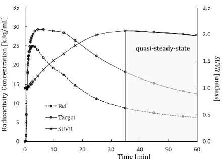
5.1 Choice of SUVR as Outcome Parameter of Interest ...91
5.2 Clinical Data ...93
5.2.1 Clinical SUVR ...93
5.2.2 Clinical 1TCM Parameters ...94
5.3 Determination of Representative Lipophilicity & Validation of In Silico fP-fND model.97 5.4 Scaling Factors ... 100
5.5 Correlation with Three Types of SUVR ... 105
5.6 Choice of Time Window ... 108
5.7 Input Function ... 111
5.8 Final Amyloid Biomathematical Model ... 116
5.9 Evaluation of Amyloid Biomathematical Model ... 119
5.9.1 Sensitivity Analysis ... 120
5.9.2 Noise Simulations ... 123
5.9.3 Effect of Input Functions ... 126
5.10 Summary ... 127
Chapter 6 ... 129
Screening Methodology of Amyloid Radiotracers ... 129
6.1 Existing Evaluation Methods ... 129
6.1.1 Coefficient of Variance (COV) ... 130
6.1.2 Receiver Operating Characteristics (ROC) ... 130
6.1.3 Power & Sample Size Analysis ... 132
6.2 Screening Methodology ... 133
6.2.1 Simulation with Population Variation & Noise ... 134
6.2.2 Clinical Usefulness Index (CUI) ... 135
6.2.2.1 Determination of Parameters ... 136
6.2.2.2 Evaluation of Parameters ... 137
6.2.3 Overview of Screening Methodology ... 140
vi
6.3.1 Screening Results ... 142
6.3.2 Comparison Data of Clinically-Applied Radiotracers ... 142
6.3.3 Evaluation of CUI ... 144
6.4 Evaluation of Effects of Input on CUI ... 146
6.4.1 Effect of KD on CUI ... 147
6.4.2 Effect of Input Function on CUI ... 148
6.4.3 Effect of Time Window on CUI ... 149
6.4.4 Effect of Scaling Factor on CUI ... 150
6.5 Limitations of Screening Methodology with CUI ... 152
6.6 Summary of Use of CUI ... 154
6.7 RSwCUI Software ... 154
6.8 Summary ... 158
Chapter 7 ... 159
Extending Screening Methodology to Tau ... 159
7.1 Tau Radiotracers ... 159
7.1.1 Issues with Existing Clinically-Applied Tau Radiotracers ... 159
7.1.2 Chirality and Stereoisomers ... 160
7.1.3 R-S Enantiomers ... 162
7.2 In Vitro & In Vivo Data of Tau Radiotracers ... 163
7.2.1 In Vitro Data of Tau Radiotracers ... 163
7.2.2 Clinical Data of Tau Radiotracers ... 167
7.3 Screening of Tau Radiotracers ... 167
7.3.1 Comparison of 1TCM Kinetic Parameters ... 169
7.3.2 Comparison of SUVR ... 170
7.3.3 Comparison of TACs and SUVR distributions ... 172
7.3.4 CUI Results of Tau Radiotracers ... 175
7.4 Summary ... 177
Chapter 8 ... 179
Overall Conclusions and Future Directions ... 179
Bibliography ... 181
Conference and Journal Papers ... 200
Journal Papers ... 200
International Conference / Symposium Presentations ... 200
vii
List of Figures
Figure 1.1: Molecular sensitivity and spatial resolution of various imaging modalities ... 2
Figure 1.2: Conventional radiotracer development process. ... 3
Figure 2.1: Amyloid precursor protein and formation of Aβ plaques ...10
Figure 2.2: Various forms of tau protein and neurofibrillary tangles. ...13
Figure 2.3: Changes in the magnitude of various biomarkers with AD progression. ...19
Figure 2.4: Various dementia diseases involving Aβ and/or Tau. ...20
Figure 2.5: Different binding sites (BS) on Aβ protein ...23
Figure 3.1: Image of a PET scan with details of positron-emission annihilation ...30
Figure 3.2: Effects of attenuation, scatter and random. ...32
Figure 3.3: Process flow of acquisition, reconstruction and processing of PET Data ...35
Figure 3.4: One tissue, two-tissue and three-tissue compartmental models ...37
Figure 3.5: Renkin and Crone Model ...40
Figure 3.6: The blood-brain-barrier (BBB). ...41
Figure 3.7: Free drug hypothesis...42
Figure 3.8: Overview of Guo’s CNS biomathematical model. ...43
Figure 3.9: Overview of Schafer & Kim’s 4TCM biomathematical model. ...47
Figure 4.1: Chemical structures of 12 clinically-applied amyloid radiotracers. ...59
Figure 4.2: Chemical structures of 29 candidate amyloid radiotracers. ...60
Figure 4.3: Maurer & Wan: fND vs. CLogP and fP vs. fND ...68
Figure 4.4: Guo: fND vs. CLogD and fP vs. fND ...69
Figure 4.5: Summerfield: fND vs. CLogP and fP vs. fND...69
Figure 4.6: Kalvass: fND vs. XLogP3 and fP vs. fND...70
Figure 4.7: A typical occupancy curve. ...79
Figure 4.8: A typical Scatchard Plot. ...80
Figure 4.9: A typical occupancy curve for competition binding assay. ...80
Figure 4.10: A Scatchard Plot showing binding to multiple binding sites. ...81
Figure 4.11: Procedures for “Sandwich” ELISA ...82
Figure 5.1: Quasi-steady-state of time activity curves of target and reference regions.. ...92
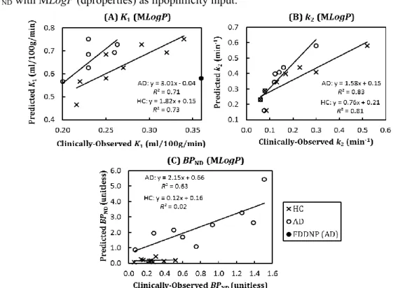
Figure 5.2: MLogP (dproperties): Correlations of predicted & clinically-observed values of K1, k2 and BPND in HC & AD. ...98
Figure 5.3: LogD+S (MedChem): Correlations of predicted and clinically-observed values of K1, k2 and BPND in HC & AD ... 100
viii
Figure 5.4: SF-AD: Correlations between predicted & clinically-observed K1, k2 and BPND in HC &
AD. ... 102
Figure 5.5: SF-HC: Correlations between predicted & clinically-observed K1, k2 and BPND in HC & AD ... 103
Figure 5.6: Time activity curves of [11C]PIB simulated using three scaling factors ... 104
Figure 5.7: Correlations of predicted SUVR with 3 types of clinically-observed SUVR ... 106
Figure 5.8: Correlations of predicted SUVR with 3 types of clinically-observed SUVR (n = 9) ... 106
Figure 5.9: Correlations of predicted SUVR using SF-AD & SF-Guo ... 108
Figure 5.10: Correlations of predicted SUVR with clinically-observed SUVR of white matter region under HC and AD conditions. ... 108
Figure 5.11: Ratio of predicted SUVRAD/SUVRHC of 5 different time windows ... 109
Figure 5.12: Correlation of predicted SUVR generated using 5 different time windows against clinically-observed SUVR under AD condition... 111
Figure 5.13: The logarithmic input functions of BF227-HC, BF227-AD, FACT-HC, FACT-AD and FDDAA with time... 112
Figure 5.14: Correlations of clinically-observed SUVR with SUVR predicted using 5 different input functions... 113
Figure 5.15: Time activity curves of [11C]PIB simulated using the 4 different input functions. ... 114
Figure 5.16: Simulated time activity curves of the reference region and target regions of HC, MCI and AD of 11 clinically-applied amyloid radiotracers ... 115
Figure 5.17: Overview of Final Amyloid Biomathematical Model. ... 116
Figure 5.18: %SUVR difference from reference with ±20% variations in MLogPonly. ... 121
Figure 5.19: %SUVR difference from reference with ±20% variations in Vx only... 121
Figure 5.20: %SUVR difference from reference with ±20% variations in fP only. ... 121
Figure 5.21: %SUVR difference from reference with ±20% variations in fND only. ... 122
Figure 5.22: %SUVR difference from reference with ±20% variations in Bavail only. ... 122
Figure 5.23: %SUVR difference from reference with ±20% variations in KD only. ... 122
Figure 5.24: Boxplots of % mean SUVR difference generated using BF227-AD, FACT-AD, FACT-HC and FDDAA from that generated using reference input function of BF227-HC under (A) HC, (B) MCI and (C) AD conditions. ... 127
Figure 6.1: Receiver Operating Characteristic. ... 131
Figure 6.2: Simulated SUVR distributions across HC, MCI and AD conditions for [11C]PIB and [18F]flutemetamol. ... 135
Figure 6.3: SUVR distribution across HC, MCI and AD conditions using poor, average and good radiotracers ... 136
ix
Figure 6.4: Es (Glass’s Delta) Vs. Es (Cohen’s D) ... 138
Figure 6.5: Correlations between Az and CL. ... 138
Figure 6.6: Relationship between CL and Es (Cohen’s D) ... 139
Figure 6.7: Overview of screening methodology for amyloid radiotracers ... 140
Figure 6.8: CUI distribution of 31 amyloid radiotracers ... 143
Figure 6.9: Relationships between 𝐴𝑧, 𝐸𝑠, 𝑆𝑟 and CUI ... 145
Figure 6.10: Relationship of the strengths of Az, Es and Sr. ... 146
Figure 6.11: CUI values generated using original KD values and ±20% change in KD values ... 147
Figure 6.12: %COV of CUI values generated using 4 different input functions ... 148
Figure 6.13: CUI distributions generated using literature-stated time window and default time window of 40-60 min. ... 149
Figure 6.14: CUI distribution of 31 amyloid radiotracers, simulated using SF-HC SF-Guo ... 152
Figure 6.15: Logo of RSwCUI software. ... 154
Figure 6.16: RSwCUI GUI: Overview ... 155
Figure 6.17: RSwCUI GUI: Results ... 157
Figure 6.18: RSwCUI GUI: CUI distribution ... 157
Figure 7.1: Classifications of chemical compounds. ... 161
Figure 7.2: Chemical structures of 22 tau radiotracers. ... 164
Figure 7.3: Correlation of clinically-observed and predicted SUVR using default time window of 40-60 min ... 171
Figure 7.4: Correlation of clinically-observed and predicted SUVR using literature-stated time window ... 171
Figure 7.5: Simulated TACs from 0–90 min of the reference region and target regions of HC, MCI and AD of 9 clinically-applied tau radiotracers ... 174
Figure 7.6: Simulated SUVR distributions across HC, MCI and AD conditions for [18F]THK523, [18F]THK5117, [18F]T807 and [11C]PBB3. ... 175
x
List of Tables
Table 2.1: Braak and Braak staging of amyloid and tau ...14
Table 2.2: The Delacourte staging of tau distribution ...15
Table 2.3: Diagnosis of clinical conditions based on diagnostic criteria ...17
Table 3.1: Commonly-applied positron emitting isotopes in PET studies ...30
Table 4.1: Overview of 10 different in silico lipophilicity models (8 LogP and 2 LogD) ...55
Table 4.2: In vitro lipophilicity values of 41 amyloid radiotracers extracted from the literature. ...61
Table 4.3: In silico lipophilicity values of 41 amyloid radiotracers generated using 10 lipophilicity models ...62
Table 4.4: Comparison of 10 in silico lipophilicity models ...64
Table 4.5: In silico and in vitro LogP of [11C]PIB and its analogues ...65
Table 4.6: Measured fP of [11C]PIB, [18F]flutemetamol & [11C]MeS-IMPY ...75
Table 4.7: Recovery, NSB, ultrafiltrate volume ratio and fP measured using ultrafiltration ...76
Table 4.8: Concentrations of Aβ1-40 and Aβ1-42 (pmol/g of tissue) measured via ELISA ...85
Table 4.9: Compiled KD or Ki values extracted from literature ...89
Table 5.1: 3 types of clinically-observed SUVR of 11 clinically-applied amyloid radiotracers. ...95
Table 5.2: Clinically-observed K1, k2 and BPND of 11 clinically-applied amyloid radiotracers. ...96
Table 5.3: In silico MLogP (dproperties) of 11 clinically-applied amyloid radiotracers. ...97
Table 5.4: In silico LogD+S (MedChem) of 11 clinically-applied amyloid radiotracers. ...99
Table 5.5: Ratio of predicted SUVRAD/SUVRHC generated using 5 different time windows. ... 110
Table 5.6: % difference of predicted SUVR from clinically-observed SUVR for HC & AD conditions. ... 110
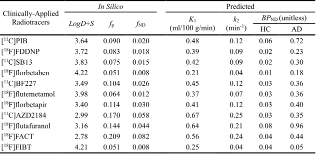
Table 5.7: Final values of in silico MLogP, Vx, fP and fND of 31 amyloid radiotracers. ... 119
Table 5.8: %COV of SUVR generated with noise simulation for 31 amyloid radiotracers under HC, MCI and AD conditions. ... 125
Table 6.1: Classification of subjects based on diagnostic test results and the actual outcome... 130
Table 6.2: Sensitivity and specificity of five clinically-applied amyloid radiotracers. ... 132
Table 6.3: Minimum, maximum, spread, mean and standard deviation of the respective parameters, Az, Es, cEs, Sr, Az x Es, Az x cEs, Es x Sr, cEs x Sr, Az x Sr and Az x Es x Sr. ... 140
Table 6.4: Az, Es and Sr of conditions-pairs of HC-MCI and MCI-AD and CUI ... 144
Table 6.5: % difference in CUI values generated using default time window from that of literature stated time window. ... 149
Table 6.6: Averaged Az, Es, Sr and CUI calculated from SUVR simulated using SF-HC & SF-Guo. ... 151
xi
Table 7.1: Basic chemical bond symbols ... 162 Table 7.2: MLogP, Vx and KD values of 22 tau-related radiotracers. ... 165
Table 7.3: Measured tau concentrations under HC, MCI and AD conditions from the literature. .... 166 Table 7.4: 3 types of clinically-observed SUVR of 8 clinically-applied tau radiotracers ... 168 Table 7.5: Predicted K1, k2, BPND and SUVR of 9 clinically-applied tau radiotracers. ... 168
xii
Abbreviations
1TCM 1-Tissue-Compartment Model AD Alzheimer’s Disease
ADL Activities of Daily Living
ADRDA Alzheimer’s Disease and Related Disorders Association AIC Akaike Information Criterion
APP Amyloid Precursor Protein AUROC Area under ROC curve Aβ Amyloid-Beta Protein BACE β-secretase
BBB Blood-Brain-Barrier BP Binding potential
BS Binding site
CAA Cerebral Amyloid Angiopathy CBF Cerebral Blood Flow
CDR Clinical Dementia Rating CIP Cahn-Ingold-Prelog CNS Central Nervous System CSF Cerebrospinal Fluid
CT Computed Tomography
DSM Diagnostic and Statistical Manual of Mental Disorders
EIA Enzyme Immunoassay
ELISA Enzyme-Linked Immuno-Sorbent Assay
FA Formic acid
fMRI Functional MRI
FP False Positive
FP False Negative
GUI Graphical User Interface
HC Healthy Control
HITP Heparin-induced tau polymer IWG International Working Group
kDa Kilo-Dalton
xiii LOR Line-Of-Response
MAP Microtubule-Associated Proteins MCI Mild Cognitive Impaired MMSE Mini-Mental State Examination MoCA Montreal Cognitive Assessment MRI Magnetic Resonance Imaging
MRTM0 Original multilinear reference tissue model NFT Neurofibrillary tangles
NIA-AA National Institute on Aging–Alzheimer's Association
NINCDS National Institute of Neurological and Communicative Disorders and Stroke NSB Non-specific binding
PBS Phosphate Buffer Saline PCG Posterior Cingulate Gyrus PET Positron Emission Tomography P-gp P-glycoprotein
PHF Paired-Helical Filament PMT Photon-Multiplier Tube PVE Partial Volume Effect rCBF Regional CBF
ROC Receiver Operating Characteristics ROI Region of Interest
SC Schwarz Criterion SDS Sodium Dodecyl Sulfate
SF Scaling Factor
sMRI Structural MRI SNR Signal-to-Noise Ratio SP Senile Plaques
SPECT Single Photon Emission Computed Tomography TAC Time Activity Curve
TN True Negative
xiv
Nomenclature
1-β Power %
ALogP Ghose-Crippen Atom-based LogP unitless
AUC Area under curve varies
Az Area under ROC unitless
Bavail.Aβ Concentration of free Aβ lesion binding sites M
Bavail.NS Concentration of free non-specific binding sites in brain tissue M
Bavail.τ Concentration of free τ lesion binding sites M
Bmax Maximum target density M
Bmax.Aβ No of binding site on Aβ proteins that can be bound per mole of radiotracer
mol of Aβ/mol of radiotracer
BPND Binding potential unitless
BSA Body surface area m2
BW Body weight kg
CFT Concentration of free ligand in brain tissue compartment M
CI Confidence interval %
CLogP /
CLogD
Calculated LogP / LogD unitless
CNS Concentration of non-specific binding sites occupied by ligand M
COV Coefficient of variation unitless
CP Plasma ligand concentration M
CReference Radioactivity concentrations in reference region kBq/mL
CS. τ Concentration of τ lesion binding sites occupied by ligand M
CS.Aβ Concentration of Aβ lesion binding sites occupied by ligand M
CTarget Radioactivity concentrations in target region kBq/mL
CUI Clinical usefulness index unitless
D Distribution coefficient unitless
DVR Distribution volumes ratio unitless
eK Distribution of errors unitless
Es Effect size unitless
f Fractional occupancy unitless
f Perfusion mL/cm3/min
xv
fp Free fraction in plasma unitless
fP Free fraction of ligand in plasma unitless
IC50 Inhibitory concentration M
IF Dynamic metabolite-corrected plasma input function (used in Guo’s model)
kBq/mL
K1 Influx rate constant mL/cm3/min
k2 Efflux rate constant min-1
KD Dissociation constant M
KD.Aβ Dissociation constant of radiotracer in specific Aβ binding compartment
M
KD.NS Dissociation constant of radiotracer in NSB compartment M
KD.τ Dissociation constant of radiotracer in specific tau binding compartment
M
koff Dissociation rate constant min-1
Kon Association rate constant M.min-1
LogD Logarithmic of Distribution coefficient (D) unitless
LogP Logarithmic of Partition coefficient (P) unitless
LogP+S / LogD+S
LogP calculated with Simulations Plus unitless
MiLogP Molinspiration LogP unitless
MLogP Moriguchi LogP unitless
NPV Negative predictive value unitless
P Partition coefficient unitless
P Permeability cm/min
PPV Positive Predictive Value unitless
PS Permeability-surface area product cm3/min/g
r1 Association rate constant for non-specific binding in brain tissue
M-1min-1
R2 Coefficient of determination unitless
r2 Dissociation rate constant for non-specific binding in brain tissue
min-1
r3 Association rate constant for specific binding to Aβ lesions M-1min-1
r4 Dissociation rate constant for specific binding to Aβ lesions min-1
r5 Association rate constant for specific binding to τ lesions M-1min-1
xvi
Rtran Rate constant mediating transfer across the blood–brain barrier mL.min-1cm-3
S Capillary surface area cm2/g of brain
SE Standard Error unitless
Sn Standard deviation of the distribution of errors unitless
Sr SUVR ratio unitless
SUV Standardised uptake value varies
SUVR Standardised uptake values ratio unitless
TPSA Topological surface area Å2
Vaq_P Apparent aqueous volume in plasma solvent/mL of
plasma
Vaq_T Apparent aqueous volume in tissue solvent/mL of tissue
VT Volume of distribution mL.cm-3
Vx McGowan volume cm3/mol/100 or
Å3/molecule
α Significant Level %
μ Linear attenuation coefficient cm-1
σpooled Pooled standard deviation varies
*Molar (M) = moles per liter (mol/L), due to small amount used in measurements, nano-Molar (nM) is commonly applied.
1
Chapter 1
Introduction
Biomedical imaging techniques such as positron emission tomography (PET) and single photon emission computed tomography (SPECT) have been applied in drug development, diagnosis and treatment of various diseases. However, the diagnosis of diseases using PET or SPECT is limited by the availability of radiopharmaceutical agents or radiotracers.
This chapter provides an overview of molecular imaging and radiotracer development in the diagnosis of dementia, particularly Alzheimer’s disease (AD). The motivation and focus of this PhD project will be explained, as well as the structure of this thesis.
1.1
Molecular Imaging
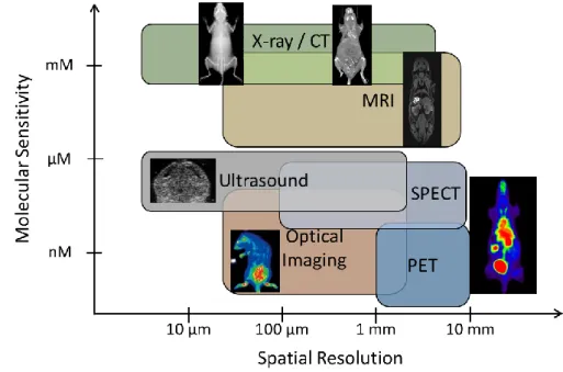
Since the 1960s, biomedical imaging has been applied to provide structural/anatomical or physiological/molecular information in animals and human in vivo. These imaging techniques rely on the detection of electromagnetic waves, such as X-rays in computed tomography (CT), radio-waves in magnetic resonance imaging (MRI), visible light in optical imaging and gamma rays in PET and SPECT, and the detection of mechanical waves such as sound waves in ultrasound (US). CT, structural MRI (sMRI) and ultrasound have high spatial resolution and are commonly used to provide in vivo structural information. Molecular imaging, on the other hand, provides non-invasive, in vivo images of the biochemical or functional processes in the living body at the molecular and cellular level. Molecular imaging technologies include optical imaging, functional MRI (fMRI), ultrasound with microbubbles, PET and SPECT. Molecular imaging modalities have poorer spatial resolution and hence are often used with structural imaging techniques in complementary to each other (Figure 1.1). For example, sMRI provides structural information at high resolution, while PET provides biological information with a radiolabeled chemical compound in a hybrid PET-MR scanner.
Molecular imaging can measure the temporal and spatial distributions of a molecular probe, which can reflect a biological process or target of interest. PET and SPECT rely on the use of a
2
radiopharmaceutical probe or radiotracer. A radiotracer is a chemical compound in which one or more atoms are replaced with a radioisotope and the detection of its decaying radionuclide allows the tracking of its location. During PET imaging, the radiotracer is injected intravenously into the subject and gamma rays emitted from the radiotracer within the body are detected by dedicated gamma detectors in a PET or SPECT scanner. The ability to detect the radiotracer has allowed the use of PET or SPECT in drug development and the diagnosis of various diseases. During drug development, the candidate drugs are radiolabeled with an isotope, with little or no change in the basic structure of the drug. Biochemical changes in the drugs, in terms of absorption, distribution, metabolism and excretion can be observed and evaluated quantitatively from the dynamic or static PET/SPECT images.
Figure 1.1: Molecular sensitivity and spatial resolution of various imaging modalities: computed tomography (CT), magnetic resonance imaging (MRI), ultrasound, single-photon emission computed tomography (SPECT), positron emission tomography (PET) and optical imaging.
Diagnostic radiotracers are radiolabeled chemical compounds developed to measure a biological function within the body (e.g. blood flow, metabolism) or to measure the concentration and distribution of certain proteins or receptors of interest (e.g. cancer cells, brain receptors). [18F]FDG (fluorodeoxyglucose), a radiolabeled analogue of glucose, is an example of a commonly-applied diagnostic radiotracer that is used to measure glucose metabolism or uptake of glucose within the body. However, unlike glucose, [18F]FDG is missing a hydroxyl group, which prevented it from being further metabolised in the cells. Therefore, it accumulates in tissues
3 with energy requirement. For example, malignant tumour cells have higher energy consumption compared to normal tissues, and hence [18F]FDG can be used in the diagnosis of cancer. Another example of a diagnostic radiotracer developed to bind to a specific target is [11C]PIB (Pittsburgh compound B), which binds to fibrillary amyloid plaques. Amyloid plaque is a pathological hallmark of Alzheimer’s disease (AD) and hence, [11C]PIB can be used to diagnose subjects, who can benefit from anti-Amyloid-beta (Aβ) treatment.
1.2
Radiotracer Development
The development of a new drug or novel radiotracer is a long, tedious and expensive process, typically taking about 10-15 years [Sharma et al., 2010] and 8-10 years [Agdeppa et al., 2009], and cost approximately USD800 million and USD150 million respectively (Figure 1.2). Thousands of chemical compounds may be screened, but only a few get selected for clinical trials, with only one compound making all the way through regulatory approval (Figure 1.2).
Figure 1.2: Conventional radiotracer development process.
The conventional process of developing a radiotracer (Figure 1.2) starts with identifying the target of interest, after which a large database of chemicals compounds are screened to determine potential chemical structures that can bind to the target of interest. The synthesis and radiolabeling of the candidate chemical compounds are designed and optimized to obtain high chemical yield while minimizing synthesis time and effort, and radioactive exposure to the radiochemists. In
4
radiotracers. Preclinical or animal testing are then followed through to determine the pharmacokinetics and pharmacodynamics of the radiotracer or drug in animals. Typically, in vitro results are first assessed, from which candidate compounds showing good results get selected for preclinical studies to minimize time and animal sacrifices.
Pharmacokinetics (PK) is the study of what the body does to the drug or radiotracer in terms of absorption, distribution, metabolism and excretion (ADME) as well as the toxicity and efficacy of the drug/radiotracer. Pharmacodynamics (PD) is the study of what the drug does to the body in terms of dose and effect. Biodistribution studies of the drug or radiotracer are important for evaluating the specific and specific binding of the drug or radiotracer to the target and non-target sites. In vitro assessments and preclinical testing are carried out iteratively until a few lead compounds are identified for further evaluation. In the case of developing a radiotracer, the feasibility and ease of radiolabeling and synthesising the compound are also considered during the development process (Figure 1.2). The procedures of radiolabeling and synthesising are optimized to reduce unnecessary radioactive exposure to radiochemist and to increase the yield of the radiotracer.
Lead compounds showing successful in vitro and/or preclinical results are selected and filed for approval for clinical studies. In drug development, phase I is conducted with a small group of healthy subjects (20~100) to evaluate safety and dosage and to identify any side effects. Phase II is carried out in a larger group of subjects (100~300), including patients to determine the efficacy of the drug and to further evaluate the safety of the drug or radiotracer. Phase III is carried in a large group of subjects (300~3000), including both healthy subjects and patients to evaluate the safety, efficacy and effectiveness of the drug or radiotracer. The use of PET and SPECT for evaluating the uptake and binding of the drug/radiotracer in vivo has allowed smaller subject groups to be evaluated in each phase, hence speeding up the development process.
However, poor bench-to-bedside translation often results due to the differences between in vitro and in vivo conditions. Similarly, animal models, especially rodents, are often poor predictors of human physiology and treatment response and have been reported to be incorrect in approximately one out of three cases [Garner et al., 2006]. Although larger animals (e.g. pigs and primates) showed closer physiology to that of human, they are still in-prefect human models and are more costly for high-throughput screening compared to rodents. These issues lead to high attrition rates in drug and radiotracer development.
5 To address these issue, the Food and Drug Administration (FDA, USA) had initiated a concept known as “Microdosing” using PET or SPECT imaging in 2006. In microdosing, a small group of healthy subjects (<10) is given a dose of no greater than 100 μg (for small molecules) or 1/100 of the No Observed Adverse Effect Level (NOAEL), whichever is the lower [Burt et al., 2016]. Preclinical testing is still required but the number of animals required for clinical approval is reduced, hence reducing the cost. Due to the low exposure of the drug or radiotracer, no gross effect, therapeutic effect, toxic effect or high radiation are expected in the subjects. However, microdosing cannot be used for therapeutic or diagnostic decision making or for safety or efficacy studies as the results may not be linearly related to full dose studies [Burt et al., 2016]. Nevertheless, the results can still be used to support candidate selection and dosage identification in Phase I studies.
The introduction of microdosing has helped to speed up the clinical Phase I studies but phases from compound screening to lead optimisation (Figure 1.2) still continue in the same laborious fashion. Development guides, such as the Rule of Five (Ro5) [Lipinski et al., 2004] provide a list of physicochemical parameters and their associated range of values for increasing the chances of developing successful drugs (e.g. molecular weight < 500 kDa, lipophilicity < 5). However, a compound that meets all the criteria of Ro5 does not guarantee that the compound will be successful [Lipinski et al., 2004]. Computational models have been introduced using different databases of chemical compounds to assist the development of new compounds (section 3.4). However, no standards have been established and only models of known targets are available.
1.3
Motivation
Dementia is a group of brain diseases, with 100 different conditions involving impairments of cognition, function & memory. Dementia patients show clinical symptoms such as memory loss, confusion in time and place etc., and subsequent decline in functional capabilities, such as the ability to eat by themselves or to change their clothes. Among the various types of dementia, Alzheimer’s disease (AD) is the most common, accounting for 60~70% of all dementia cases worldwide. The number of dementia cases is increasing every year, which leads to an increasing cost of care for dementia patients. Early detection of the disease will increase the success rate of treating AD or slow down the rate of dementia. Since 2000, many institutions have tried to develop amyloid and tau-targeting radiotracers to assist diagnosis of AD and support AD drug
6
development. However, up to date, only three amyloid radiotracers and no tau radiotracers had been approved by FDA (section 2.2.3).
The development of a successful diagnostic radiotracer is hampered by the limitations of the conventional radiotracers development process. Firstly, it is a long and iterative process of identifying the right chemical compounds, followed by lead optimisation via iterative processes of conducting multiple in vitro experiments and preclinical testing before the radiotracer can be applied clinically. Secondly, in vitro and preclinical results may not translate well to clinical performance, due to the lack of consideration to the possible in vivo kinetics of the radiotracers. Radiotracers with poor kinetics may not show much differences in the in vivo uptake under different subject conditions. Thirdly, the conventional process focuses on a few physicochemical or pharmacological properties (e.g. lipophilicity, selectivity to target sites) to evaluate radiotracer. These properties are often evaluated separately, without considering their interaction effect. Lastly, the noise level of the imaging modality and target variation are either not considered or evaluated separately during radiotracer development.
Biomathematical simulation can complement high-throughput screening by allowing simultaneous and rapid evaluation of many candidate radiotracers. Moreover, the radiotracers can be evaluated by using both physicochemical and pharmacological parameters to simulate their possible in vivo kinetics at variable conditions. The statistical evaluation of the radiotracers can also be increased by simulating with noise and population variation. To further support decision-making in moving candidate radiotracers for clinical evaluation, the use of a common index can support comparison of different radiotracers from within and across institutions. As such, biomathematical simulation can help to identify potential compounds from a large number of compounds during the early phrase of drug development, especially before radiolabeling of candidate radiotracers (Figure 1.2). This will help to reduce the number of in vitro experiments and radiolabeling procedures and hence speed up the radiotracer development process and reduce radioactive exposures to the radiochemists.
At cyclotron and radioisotope center (CYRIC) in Tohoku University, we are actively developing amyloid and tau radiotracers in hope to support the diagnosis of AD and to assist AD drug treatment. As such, we would like to develop a screening methodology using biomathematical simulations to support the screening process of chemical compounds during the development of amyloid and tau radiotracers, especially during the design of new candidate compounds before
7 the synthesis and radiolabeling of the candidate compounds (section 1.2). This will help to reduce the radioactive exposure to radiochemists while supporting the screening of thousands of compounds more efficiently with the consideration of the possible in vivo kinetics of the radiotracers leading to higher success rate. Thus far, few models for amyloid and tau radiotracers were developed and they were developed using one or a few radiotracers due to the unavailability of many radiotracers. Moreover, the existing amyloid and tau models were not focused on supporting radiotracer development.
We proposed to use the reported clinical data of amyloid radiotracers for the development of an amyloid biomathematical model to predict the in vivo kinetic behaviour of candidate amyloid radiotracers in HC and AD. A screening methodology based on the proposed biomathematical model will then be developed to support decision making in moving the candidate radiotracer to clinical application. We then investigate if the screening methodology can be extended to support the development of tau radiotracer.
1.4
Structure of Thesis
Chapter 1 introduces the basics of molecular imaging and the development and uses of radiotracers in drug development and diagnosis of various diseases. The motivation and structure of this thesis are explained. Relevant conferences attended and journal papers submitted during the course of PhD are listed.
Chapters 2 and 3 provide the background in the development of the amyloid biomathematical model. Chapter 2 explains the details of Alzheimer’s disease, in particular, the two pathological hallmarks of AD: amyloid and tau proteins. Existing issues in amyloid and tau imaging are discussed, as they are important in supporting the feasibility of the proposed model. Chapter 3 explains the fundamentals of positron emission tomography (PET) and quantitative analysis of PET images. Two existing biomathematical models are then described and the feasibility of extending the model for our model is debated.
Chapters 4 to 6 describe the development of the screening methodology in details. Chapter 4 focuses on determining the physicochemical and pharmacological properties of the radiotracers required in the biomathematical model. The development and evaluation of the amyloid biomathematical model are described in chapter 5. A screening methodology based on the
8
proposed amyloid biomathematical model is developed in chapter 6. A program written for screening amyloid radiotracers based on the proposed methodology is presented.
In chapter 7, we explore the feasibility of extending the proposed amyloid biomathematical screening methodology for screening tau radiotracers. We then conclude the project and my work done for this PhD project in chapter 8.
9
Chapter 2
Pathology & Diagnosis of Alzheimer’s
Disease
Amyloid and tau PET imaging can show the distribution and concentration of amyloid and tau in the subject brain. However, the amyloid and tau proteins have many different structural forms and undergo many post-translational processes, some of which lead to neurotoxic degeneration causing AD, while some do not. In this chapter, the different forms of amyloid and tau proteins are described in details to ensure that the right information is selected for model development. The diagnosis of AD using other biomarkers and classification of subjects based on various diagnostic criteria standards and neuropsychological tests are briefly described followed by two staging methods of AD based on concentration and spatial distribution of amyloid and tau in the brain. Clinically-applied amyloid and tau radiotracers are presented and the existing issues faced in clinical amyloid and tau PET imaging are discussed.
2.1
Alzheimer’s disease
Alzheimer’s disease (AD) is a progressive neurodegenerative disorder defined by histopathological features such as senile plaques (SP) and neurofibrillary tangles (NFT) [Perrin et al., 2009] and clinical symptoms such as loss of memory, reduced executive functions etc. AD was discovered and named after Alois Alzheimer, a German physician in 1906, who examined a patient exhibiting memory loss, language difficulty and confusion. When the patient died at the age of 51, he carried out post-mortem brain autopsy and observed SP and NFT in her brain tissues. [Stelzmann et al., 1995]. These subsequently became the pathological hallmarks of AD.
In this section, the structure and biological development of SP and NFT from Aβ and tau proteins are described in details, in particular, the in vitro method of identifying Aβ and tau proteins. The spatial and temporal distributions of Aβ and tau proteins in 2 staging methods with AD progression are also explained.
10
2.1.1
Amyloid-Beta Protein
The component of senile plaques was unknown at the time of discovery by Dr Alzheimer. It was only in 1984 that Aβ was discovered when it was successfully purified from the senile plaques [O’Brien et al., 2011]. Aβ peptide is cleaved from the amyloid precursor protein (APP), which is a transmembrane protein of ~100-130 kDa (kilo-Dalton), with a maximum of 770 amino acids (Figure 2.1A). The APP is located on the plasma membrane, trans-Golgi network, endoplasmic reticulum and endosomal, lysosomal and mitochondrial membrane. As such, Aβ peptide can be found intracellularly and extracellularly. The physiological functions of APP are still unconfirmed but are proposed to relate to cell growth and neuronal plasticity.
Figure 2.1: (A) Amyloid precursor protein (APP) [O’Brien et al., 2011] and (B) formation of Aβ plaques [Morgan et al., 2004].
Three main proteases are involved in the proteolytic cleavage of APP, namely α-secretase, β-secretase (or BACE) and γ-β-secretase. They act in pairs to form the amyloidogenic and non-amyloidogenic peptides. Non-non-amyloidogenic peptides are first cleaved by the α-secretase at the N-terminal, followed by γ-secretase at the C-terminal of APP (Figure 2.1A). The amyloidogenic peptides or Aβ peptide are first cleaved by the β-secretase at the N-terminal, followed by
γ-11 secretase at the C-terminal (Figure 2.1A).
Aβ is a small peptide of about 4.2 kDa and consists of 37 to 43 amino acids (Figure 2.1B) [O’Brien et al., 2011]. Aβ1-37 to Aβ1-40 are known as the benign forms, while Aβ1-42/43 are known as the toxic forms [Karran et al., 2011]. The most common forms of Aβ peptides are Aβ1-40/42, of which Aβ1-42 was reported to polymerise more readily than Aβ1-40. The different types of Aβ proteins exist in varying degree in different cellular compartments, namely intracellular, extracellular and membrane surface) [Steinerman et al., 2008].
A single Aβ peptide, also known as a monomer, can join together to form longer and more toxic peptides such as dimer, trimer, and tetramer. These peptides undergo oligomerization to form a soluble oligomer or insoluble fibrillary Aβ (Figure 2.1B). Soluble forms are soluble in aqueous solution and remain soluble even after high-speed centrifugation. The concentrations of soluble Aβ and insoluble Aβ peptides are about 6 and at least 100 times respectively higher in AD brains than in normal brains [Morgan et al., 2004]. These oligomers undergo further post-translation modifications (e.g. truncation, racemization, oxidation, polymerization) to form large Aβ deposits. Three types of amyloid-beta (Aβ) deposits can be found in the human brain, namely senile/neuritic plaques, diffuse plaques and cerebrovascular amyloid (Figure 2.1B) [Morgan et al., 2004]. Senile plaques are large extracellular aggregates of Aβ consisting of a dense central fibrillary Aβ core filled with inflammatory cells and dystrophic neurites or dendrites, containing tau in its periphery [O’Brien et al., 2011]. They are known as the cause of AD. Senile plaques have high concentrations of Aβ1–42, which are subjected to post-translational modifications including oxidation, oligomerization and polymerization. They have pleated β-sheet structure, which is strengthened by hydrogen bonds formed between the Aβ peptides. Senile plaques can be identified by fluorescent dyes, such as Thioflavin-S/T and Congo-Red.
Diffuse plaques are amorphous and non-neuritic amyloid deposits, which are commonly found in the brains of cognitively intact elderly people. They do not β-sheet structure, thus they can only be identified by modified silver methenamine methods. Cerebrovascular amyloid consists of Aβ peptides, mainly Aβ1-39/40/42, deposited in cerebral blood vessels and are spared from post-translational modifications (Figure 2.1B). It forms the main component of cerebral amyloid angiopathy (CAA). The soluble oligomer is said to be the cause of neurotoxic instead of fibrillary senile plaques: the prefibrillar soluble Aβ oligomer may induce toxic effect leading to cell death
12
or the diffuse plaques may unfold and reorganise into senile plaques, during which toxic is release leading to cell death (Figure 2.1B).
2.1.2
Tau Protein
Tau proteins belong to the microtubule-associated proteins (MAP) family. They are normally present in the axon and plays a part in axonal transportation and stabilisation of the microtubules [Buĕe et al., 2000]. The tau structure consists of two domains – projection and microtubule-binding domains (Figure 2.2A) [Buĕe et al., 2000]. The projection domain consists of the acidic and basic regions, with the N-terminal (amino terminal). The microtubule-binding region consists of the repeat-domain and neutral regions, with the C-terminal (carboxy-terminal). A total of six isoforms of tau proteins exist. They differ in the number of exons (0, 1, 2) on the acidic region and the number of repeats (3 repeats (3R) or 4R) in the repeat-domain regions (Figure 2.2A). The R1-R2 region exists only in 4R tau (Figure 2.2A) and is the main cause for the 40 times difference in binding affinities to microtubules between 4R and 3R tau [Buĕe et al., 2000]. They are made up of about 352~441 amino acids, with a molecular weight ranging from 45 to 65 kDa [Buĕe et al., 2000]. The shortest isoform, known as the fetal isoform, is found only in the fetal brain. The rest of the isoforms are known as the adult isoforms. In normal adults, the proportion of 3R and 4R tau is nearly equal, but in AD, the proportion of 4R is much higher than 3R.
Tau proteins undergo many post-translational modifications, of which phosphorylation plays the key role in determining the binding with microtubules (Figure 2.2B). Tau protein undergoes phosphorylation under normal ageing, forming highly soluble phosphorylated tau that does not form filamentous inclusion. However, under abnormal conditions, hyperphosphorylation occurs, yielding intraneuronal filamentous, insoluble inclusions called paired-helical filament (PHF) tau, which consists of a pleated β-sheet structure. A small amount of tau may form other types of ultra-structures, such as straight-like filaments, twisted filaments, randomly coiled filaments or hybrid filament, which has a sharp change from straight to helical structure [Serrano-Pozo et al., 2011].
Further aggregation of PHF-tau results in neurofibrillary tangles (NFT), which consists of 3 morphological stages (Figure 2.2B): (1) Pre-NFT, with a more diffuse structure, (2) Intraneuronal NFT (iNFT), with matured or fibrillary structure, and (3) extraneuronal NFT (eNFT) [Serrano-Pozo et al., 2011]. eNFT is also known as “ghost” tangle, as it results from the death of tangles-containing neurones. It can be identified by the lack of a nucleus and the presence of a stainable
13 cytoplasm due to the breakdown of the cell membrane [Serrano-Pozo et al., 2011]. Although NFT is said to be toxic, the tau form that leads to neurotoxicity is still being debated. Some have proposed that the soluble tau, which is formed before hyperphosphorylation to form PHF-tau under abnormal conditions, is toxic or both NFT and soluble tau lead to cell death via different routes [Kopeikina et al., 2012].
Figure 2.2: Various forms of tau protein: (A) 6 isoforms of tau protein [Ariza et al., 2015], (B) Aggregation of tau protein to neurofibrillary tangles.
NFT are argyrophilic (readily stained by silver salts) and can be identified in vitro by silver staining methods (e.g. Gallyas technique) or fluorescent staining or immunostaining using anti-tau antibodies (e.g. AT8 and PHF1 for i/eNFT, MC1 and Alz50 for Pre-NFTs) [Serrano-Pozo et al., 2011]. Fluorescent dyes, such as Thioflavin-S/T and Congo-Red, bind to structures with β-sheet conformation and hence can be used to detect PHF-tau. Apart from NFT in cell bodies, phosphorylated tau can exist as neuropil threads in dystrophic neurites or in the neuropil.
14
Synthetic heparin-induced tau polymer (HITP) generated in vitro composed of 3R and/or 4R tau and does not undergo the same phosphorylation process under in vitro conditions [Ariza et al., 2015]. Moreover, synthetic tau phosphorylates to form homogeneous or granular structure instead of fibrillary structure found in human [Buĕe et al., 2000; Declercq et al., 2016]. In transgenic mouse model expressing human recombinant tau, only 4R tau isoforms are expressed, but in human AD brains, both 3R and 4R are expressed [Declercq et al., 2016]. As such, in vitro and pre-clinical results of tau radiotracers do not translate well into clinical results.
2.1.3
Distributions of Amyloid & Tau
The spatial distributions of amyloid and tau proteins in postmortem brains of healthy and AD subjects have been extensively studied since 1990 especially by Braak and Braak [Braak et al., 1991] and Delacourte [1999]. Both groups have tried to study the spatial and temporal distributions, and changes in the concentrations of amyloid and tau proteins to stage the pathological progression of AD.
Braak et al. staged AD progression based on the histopathological distributions of amyloid and tau proteins separately using 2661 normal and AD brains from 1991 to 1997 [Braak et al., 1997]. Amyloid and tau proteins were identified using silver-pyridine and silver-iodide staining respectively. Braak et al. [1991] managed to stage the amyloid and tau accumulation and distributions into 3 (A-C) and 6 (I-VI) stages accordingly (Table 2.1).
Table 2.1: Braak and Braak staging of amyloid and tau Amyloid Stages A-C
Stage A: Lingual and fusiform gyri (medial and lateral occipito-temporal gyri = basal temporal neocortex) Stage B Basal Cortex
Stage C: Upper portions of the cortex & the primary neocortical areas + Cerebellum Tau Stages I-VI
Stage I Transentrohinal region (Temporal Lobe) Stage II + Entorhinal region
Stage III +Hippocampal & Temporal preneocortex Stage IV + Adjoining neocortex
Stage V Spread Superolaterally Stage VI Primary Neocortex
15 distribution and severity of cognitive impairment evaluated using 2 clinical assessments: Mini-mental state examination (MMSE) and clinical dementia rating (CDR). Aβ was identified using thioflavin-S and antibodies against Aβ. Tau proteins were identified using silver staining (Bielchowski) and antibodies against tau. Delacourte et al [1999] managed to stage AD progression based on tau distribution in ten stages using 130 brains (Table 2.2). However, there was a rare case where an elderly brain with severe cognitive impairment had low concentrations of tau distributed throughout the brain.
Table 2.2: The Delacourte staging of tau distribution Stages Regions Subjects No of (Mean ± Stdev) Age Aβ Density (pmol/mg)
(Subj No) Cognitive Status & notes
I Trans-entorhinal 3 71~83 (77 ± 6) 0 All were Non-Demented
II +Entorhinal 4 72~95 (86 ± 10) Low (2) 2 without dementia (incl 95-years-old) III +Hippocampus 16 73~95 (84 ± 7) 10 (2), 20 (3) 6 vascular demented, 4 ND IV temporal cortex +Anterior 10 69~98 (88 ± 9) 11 (max) 5 ND, 4 MCI; 2pmol/mg Aβ in 98-years-old
V +Inferior temporal 12 76~98 (89 ± 7) 0 (2), 20 (3), 30 (1) 3 ND, 3 vascular demented
VI +Mid-temporal 11 71~93 (86 ± 7) 54 (1) 0 (1), 1 ND (88-years-old), rest with moderate Aβ load VII superior temporal, +Anterior frontal,
inferior parietal 15 84~106 (96 ± 6) High
1 ND (84-years-old, with low tau conc.), 4 (ND or MCI, low tau conc.) VIII +Broca area 5 77~91 (87 ± 6) low~high All demented 88 (2),
IX +Motor cortex 19 65~100 (81 ± 8) 10~200 All demented
X +Occipital areas 27 37~90 (74 ± 13) - Highest tau conc. in temporal cortex From the results of both Braak and Braak [1991 and 1997] and Delacourte [1999], tau was found in the brains of young subjects and in the absence of Aβ. In addition, the hippocampal region was shown to be a vulnerable region to tau degeneration. The deposition of Aβ was more widespread with no consistent pattern except for increasing densities in various regions, while tau deposition is progressive and ordered, following along precise anatomic networks. Although Aβ and tau coexist in late stages of AD, they do not correlate well with each other. Although tau concentrations correlated well with cognitive impairment, there were a few subjects that differed from expectations in Delacourte’s results. Moreover, based on Delacourte’s staging, all subjects investigated had cognitive impairment only after the late tau stages of VII (Table 2.2). This
16
showed that tau imaging can also be used as a biomarker for early diagnosis of possible AD conversion apart from amyloid imaging.
2.2 Diagnosis of AD
Early detection of possible AD conversion will help patients benefit from early AD intervention and treatment. As the clinical symptoms of AD overlap with other dementia symptoms, it is important to discriminate the type of dementia in order to treat the patients correctly. AD diagnosis is carried out using clinical assessments and various biomarkers of AD. This section explains the various subject groups based on clinical or other assessments, as well as the biomarkers of AD, in particular, amyloid and tau imaging.
2.2.1
Clinical Diagnosis
Up to date, the only definitive diagnosis of AD is post-mortem autopsy, even then there had been conflicting results with the lack of senile plaques or low concentrations of NFT in subjects showing clinical AD symptoms. Clinical symptoms of dementia can be assessed via neuropsychological assessment, such as mini-mental state examination (MMSE) [Folstein et al., 1975], Montreal cognitive assessment (MoCA) [Nasreddine et al., 2005] and clinical dementia rating (CDR). These assessments evaluate the various cognitive domains, such as attention, memory, language, visuospatial function, and executive function. Risk factors for AD such as family history of dementia, ApoE-4 genotype and female gender are also identified during the clinical assessment.
To standardise the diagnosis of clinical conditions, diagnostic criteria have been established by different working groups. The most commonly used criteria are established by the National Institute of Neurological and Communicative Disorders and Stroke (NINCDS) and the Alzheimer’s Disease and Related Disorders Association (ADRDA) (NINCDS-ADRDA) to classify the various conditions, including AD [McKhann et al., 2011], preclinical AD [Sperling et al., 2011] and MCI [Albert et al., 2011]. Other working groups include the Diagnostic and Statistical Manual of Mental Disorders (DSM-5), International Working Group (IWG) and National Institute on Aging–Alzheimer's Association (NIA-AA). Subjects are classified into various groups based on the criteria-stated neuropsychological assessment, risk factors and/or other biomarkers. However, different diagnostic criteria defined and termed the various conditions differently (Table 2.3).
17 Two common clinical conditions are healthy control (HC), where the subject has no memory or cognitive impairment and AD, where the subject had memory, cognitive and functional impairments. With new information from clinical studies, the terms and criteria used to describe and classify the various subject conditions or states have changed over time. For example, the terms “probable/possible AD dementia” or “dementia due to AD” or “dementia of Alzheimer type (DAT)” are introduced to replace “AD” condition. This is because AD clinical conditions overlap with other dementia conditions and definitive diagnosis of AD can only be confirmed via post-mortem autopsy.
Table 2.3: Diagnosis of clinical conditions based on diagnostic criteria
Clinical Symptoms NINCDS-ADRDA DSM-5 IWG NIA-AA
No / Subtle complaints Preclinical AD - Asymptomatic AD / Presymptomatic AD Preclinical AD Cognitive impairment but functionally independence
MCI due to AD MCI due to AD Prodromal AD MCI due to AD
Dementia Dementia due to AD Probable AD AD dementia Dementia due to AD / Possible AD / Probable AD The purpose of clinical assessment is to identify subjects that are probably AD to provide correct treatment and those who are likely to convert to AD for early disease intervention. The earlier the intervention, the more effective the treatment and the faster the recovery. As such, the critical diagnosis period between pre-clinical AD and mild cognitive impairment (MCI) are very important for early diagnosis of AD.
Pre-clinical or pre-symptomatic AD condition is the state between HC and MCI, where no clinical symptoms can be observed. Mild cognitive impairment (MCI) is the clinical condition in which memory or other cognitive functions are lower than HC but the daily functioning is not hindered or not severe enough to be classified as AD. MCI can be further classified based on memory impairment (amnestic vs. non-amnestic) and the number of cognitive domains involved (single or multiple domains). Amnestic MCI have memory impairment while non-amnestic MCI do not have memory impairment but suffers from other cognitive impairment (e.g. decision-making, visual perception). As MCI is an evolving diagnostic condition, it has been further classified into
18
“MCI due to AD”, “mild AD” or “mild to moderate AD” and “prodromal AD”. Subjects classified as MCI due to AD condition have a high likelihood of converting to AD, with positive Aβ results and/or neuronal injury [Albert et al., 2011].
In our study, mild AD is considered under AD, stage I based on the results by Peterson et al. [1999] (Figure 2.3). Mild AD condition has similar memory performance as MCI conditions but other cognitive domains are more impaired than MCI [Petersen et al., 1999]. Even though some groups have classified prodromal AD as an individual state occurring before MCI, some termed it as clinical assessment of MCI, confirmed with a biomarker such as PET imaging (Table 2.3). Therefore, prodromal AD and MCI are considered under the same clinical diagnosis of MCI in our study.
2.2.2
Biomarkers of AD
Neuropsychological assessments may be limited in discriminating the various subject conditions or types of dementia due to overlapping clinical symptoms and subjective interpretation of assessment questions. Some tests like CDR have small scale range (0-3), while some tests like MMSE have large scale range (0-30). The test differed in sensitivity and specificity, as the cutoff thresholds differ for each group at different centers. Moreover, normal ageing also contributes to poorer test scores and varies with the individual, age and other factors. As such, clinical assessments are often carried out with other biological tests or imaging for more evident classification.
Existing biomarkers for AD either target Aβ deposition, tau deposition or neuronal injury (Figure 2.3). Biomarkers of Aβ deposition includes amyloid PET imaging and decrease Aβ1-42 in cerebrospinal fluid (CSF). Similarly, the biomarkers of tau deposition include tau PET imaging and increase tau in CSF (Figure 2.3). Little or no changes in CSF measurements were obtained during the progression of MCI to AD and the clinical phase of AD. Hence, unlike PET imaging CSF measurements cannot be used for staging of AD or tracking disease progression. This may be due to the sensitivity of measurement methods or due to pathology, where the discharge of amyloid and tau into CSF becomes stable. The extraction of CSF for evaluation requires invasive lumbar puncture and hence is not preferred for diagnosis especially in patient subjects. Moreover, such assessments only measure the concentrations of amyloid and tau but do not provide any spatial information of the amyloid and tau distribution in the brain. Biomarkers of neuronal injury include reduced hippocampal volume or increased rate of brain atrophy measured using MRI or
19 CT, decreased metabolism with [18F]FDG-PET imaging, and reduced blood flow via fMRI or [15O]H
2O-PET imaging etc. (Figure 2.3). Structural changes in the diseased brain can be evaluated via MRI or CT but changes can be subtle until clinical symptoms set in (Figure 2.3).
Figure 2.3: Changes in the magnitude of various biomarkers with AD progression.
Aβ = amyloid-beta, NFT = neurofibrillary tangles, CSF = Cerebrospinal fluid, ADL = Activities of daily living, Mod. = Moderate, Sev. = Severe, CDR = Clinical dementia rating.
As Aβ and tau proteins can be found in other types of dementia, amyloid and tau PET imaging can be used for differential diagnosis (Figure 2.4). Differential diagnosis is the process of differentiating two or more diseases or conditions having identical or similar symptoms or target pathologies. A group of neurodegenerative diseases, which pathologically involves tau are called “tauopathies”. AD is histopathologically defined by both amyloid and tau proteins only (Figure 2.4). All the other forms of dementia either consists of tau in specific brain regions (e.g. corticobasal degeneration (CBD)) or is also histopathologically defined together with other proteins (Figure 2.4).
Amyloid and tau PET imaging are non-invasive and allows one to measure the in vivo spatial distribution of Aβ and tau in the brain quantitatively. As amyloid load shows greater changes in the early stages of AD (Figure 2.3) [Perrin et al., 2009], amyloid imaging allows for early
![Figure 2.2: Various forms of tau protein: (A) 6 isoforms of tau protein [Ariza et al., 2015], (B) Aggregation of tau protein to neurofibrillary tangles](https://thumb-ap.123doks.com/thumbv2/123deta/5916274.1050760/32.892.143.754.324.823/figure-various-protein-isoforms-protein-aggregation-protein-neurofibrillary.webp)