Bifurcation of Transition Layers in Reaction-Diffusion Systems (International Conference on Reaction-Diffusion Systems : Theory and Applications)

(1)

Bifurcation of Transition Layers

in Reaction-Diffusion Systems

1

広島大学理学研究科坂元国望 (Kunimochi SAKAMOTO)

Graduate School ofScience Hiroshima University

Another title of this article may be:

Searching forStable Multi-Dimensional Patterns

in Reaction-Diffusion Systems.

This is astory of my research activities during the last few years, in searching for

multi-dimensional patterns for reaction-diffusion systems. As regard to stable

pat-terns, this is not a successstory. It tellsus, however, about the intricaciesonefaces in

dealing with multi-dimensionaltransition layers. In retrospect, onespace-dimension

was a fortunate exception in which there is no extra dimension for instability to set

in. As soon as the dimension of the domain becomes higher than one, instabilities

creep in to transition layers from the extra dimension along interfaces.

1. REACTION-DIFFUSION EQUATION AND INTERFACE EQUATION

1.1.

Reaction Diffusion

System. Atwocomponent system of reaction-diffusion

equa-tions, such as

(R-D) $\{$

$\frac{\partial u}{\partial t}=$ _{$d_{1}\triangle u+f(u, v)$}

$(x\in\Omega, t>0)$

$\frac{\partial v}{\partial t}=$ _{$d_{2}\triangle v+g(u, v)$}

$\frac{\partial u}{\partial \mathrm{n}}=0=\frac{\partial v}{\partial \mathrm{n}}$ _{$(x\in\partial\Omega, t>0)$}

has been widely employed to model various pattern formation phenomena $[4, 7]$. The

domain $\Omega\subset \mathbb{R}^{N}$ here is assumed to be bounded and smooth, and

$\mathrm{n}$ stands for outward

unit normal

on

$\partial\Omega$.

According to various types of nonlinearity $(f, g)$, the system above, dispite of its

sim-plicity, is capable of modelling multitude ofpatternformation phenomena. In this article,

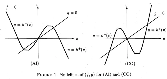
we deal with two types of nonlinearity. Prototypical examples ofthese are:

(AI) $f(u.v)=u-u^{3}-v$, $g(u., v)=u$ –v

and

(CO) $f(u., v)=u-u^{3}+v$, $g(u, v)=u$ -v.

12000.

Mathematical$\mathrm{c}\mathrm{l}\mathrm{a}\mathrm{s}\mathrm{s}\mathrm{i}\mathrm{f}\mathrm{i}\mathrm{c}\mathrm{a}\mathrm{t}\mathrm{i}\mathrm{o}\mathrm{n}\mathrm{s}:35\mathrm{B}25$

.

_{$35\mathrm{B}35,35\mathrm{K}57$}

Keywords: reaction-diffusion system, bifurcation, _{internal layer,} _{interface equation, free boundar}

数理解析研究所講究録 1249 巻 2002 年 90-102

(2)

(AI)

FIGURE 1. Nullclines of $(f, g)$ for (AI) and (CO)

When does the system (R-D) produce patterns? Here, a pattern means a spatially

inhomogeneous solution. The following theorem gives us an insight in answering this

question.

Theorem 1 (Conway-Hoff-Srrrdller [3]).There exits a positive constant $d_{0}=d_{0}(\Omega, f, g)$

such that

_if

$\min\{d_{1}., d_{2}\}>d_{0}$ then the solutions

of

(R-D) behaves approximately similar

to those

_of

the ordinary

_differential

equations

(ODE) $u_{t}=f(u.v)$, $v_{t}=g(u, v)$,

after

initial transients.

The theoremsaysthat the diffusion forces the spatial homogenization of the solution of

(R-D). In this sense, _the _diffusion _acts in accordance with our intuition, and when both

diffusion coefficients $d_{1}$ and $d_{2}$ are rather $1\mathrm{a}\mathrm{r}\mathrm{g}\mathrm{e}_{\dot{\mathit{1}}}$ the system (R-D) does not create any

pattern. This in turn suggests that one ofthe diffusion rates must be small in order for

(R-D) to produce patterns.

Therefore, we assume in the sequel that the diffusion rate $d_{1}$ of $u$ is small while $d_{2}$

remains of order $O(1)$ as $d_{1}arrow 0$:

$0<d_{1}=\epsilon^{2}\ll 1’$. $0<d_{2}=D=O(1)$ (as $\epsilonarrow 0$).

Then (R-D) is rewritten as

(1.1) $\{\begin{array}{l}u_{t}=\epsilon^{2}\triangle u+f(u,v)v_{t}=D\triangle v+g(u,v)\end{array}$ $x\in\Omega t>0$.

In (1.1) (and also in the sequel), the reference to the boundary conditions is omitted,

be-cause

we always deal with the homogeneous Neumann boundary

conditions. The

general

behavior of solutions to (R-D) with appropriate

initial conditions

$(u(x.0).v(x.0))=(u_{0}(x).v\mathrm{o}(.?\cdot))$

(3)

is

well known

[1]. For example,

if the second

component $v_{0}(x)$

of the initial condition

satisfies $|v_{0}(x)|\leq 2/(3\sqrt{3})$ for $x\in\overline{\Omega}$

, then the solution $(u(x, t),$$v(x, t))$ of(R-D) develops

internal layers

as

$tarrow\propto$.

Namely, for large $t$, $u(x.t)\approx h^{-}(v(x., t))$ for _{$x\in\Omega^{-}(t)$} and _{$u(x,t)\approx f^{+}(v(x_{\dot{J}}t))$} for

$x\in\Omega^{+}(t)$_, thus

creating

asharp transition of _$u(x,t)$ from the left

branch

_$u=h^{-}(v)$ to

the right

branch

$u=h^{+}(v)$ of the

nullclien

$\{f=0\}$ (cf. Figure 1)

near

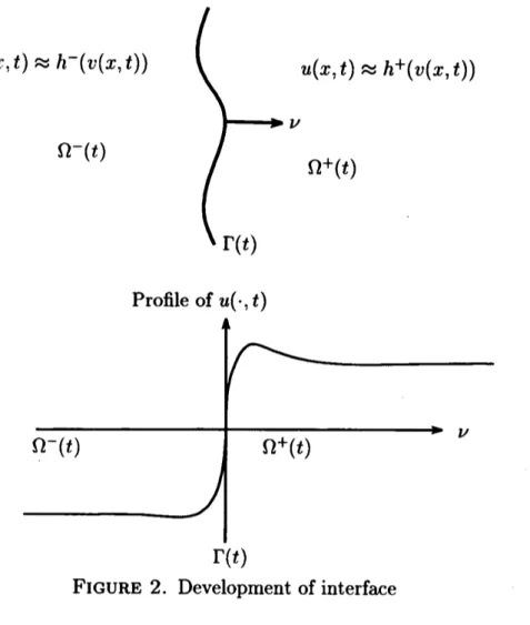
the set $\Gamma(t)$, called

interface. The development of the sharp transition layer is caused by the bistability of

$u(x.t)’\approx h^{-}(v(x,t))\Omega^{-}(t)$

$\}_{\Gamma(t)}\nu_{\Omega^{+}’(t)}u(x.t)\approx h^{+}(v(x,t))$

FIGURE

2. Development of interface

the scalarordinary differential equation

$\frac{du}{dt}=f(u_{2}v)$

which is the first equation in (R-D) with the diffusion term being neglected. Note that

$u=h^{-}(\iota,,).\prime h^{+}(v)$ are stable equilibria of the scalar ordinary differential equation for

$|v|<2/(3\sqrt{3})$.

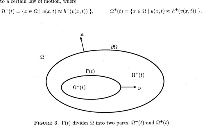
1.2. Interface Equation. When thetransition layerbecomes sosharpthat the diffusion

term $\epsilon\triangle u$ cannot be neglected, the location of the layer

$\Gamma(t)\subset\Omega$

.

called the

interface

at

$t>0$ which

divides

$\Omega$ into two regions $\Omega^{\pm}(t)$ (cf. Figure 3), starts

migrating

accordin

$\mathrm{g}$

92

(4)

to acertain law of motion where

$\Omega^{-}(t)--\{x\in\Omega|u(x, t)\approx h^{-}(v(x., t))\}$. $\Omega^{+}(t)=\{x\in\Omega|u(x, t)\approx h^{+}(v(x, t))\}$.

$\Omega$

FIGURE 3. $\Gamma(t)$ divides $\Omega$ into two parts, _{$\Omega^{-}(t)$} and $\Omega^{+}(t)$.

In order to describe the motion law., let us consider the following nonlinear eigenvalue

problem:

$\phi’(z)+c\phi’(z)+f(\phi(z), v)=0$ $(z\in \mathbb{R})$,

$\lim_{zarrow-\infty}\phi(z)=h^{-}(v).$, $\lim_{zarrow+\infty}\phi(z)=h^{+}(v)$, $\phi(0)=0$.

It is known that the problem has aunique solution pair $(\phi(z), c(v))$ for $v\in(\underline{v}_{\dot{l}}\overline{v})$. The

wave speedsatisfies:

(WS) $\{$

$d(u)>0$ for (AI)

$c’(v)<0$ for (CO)

It turns out that the sign of $c_{J}’(v)$ plays acrucial role in the following discussions.

When the $u$-component develops internal layer it is either $u(x.t)\approx h^{-}(v(x., t))$

or

$u(x, t)\approx h^{+}(v(x., t))$, on $\Omega^{-}(t)$ or $\Omega^{+}(t)$. respectively. So it is natural to define $g^{*}$ by

$g^{\mathrm{x}}(v, xj\Gamma(t))=\{$

$g(h^{-}(v), v)$ if $x\in\Omega^{-}(t)$

$g(h^{+}(v)., v)$ if $x\in\Omega^{+}(t)$.

Themotion-law of the interface under the time scale of (1.1) isdescribed bythe following

system of equations:

(1.2-a) $\mathrm{v}(Xj\Gamma(t))=0$ $(x \in\Gamma(t), t>0)$,

(1.2-b) $v_{t}=D\triangle v+g^{\mathrm{x}}(v.xj\Gamma(t))$ $(x\in\Omega\backslash \Gamma(t)., t>0).$_,

(1.2-c) $v(\cdot.t)\in C^{1}(\overline{\Omega})\cap C^{2}(\Omega\backslash \Gamma(t))$ .

(5)

In (1.2-a), $\mathrm{v}(Xj\Gamma(t))$ is the speed of $\Gamma(t)$ at $x\in\Gamma(t)$ along the unit normal vector $\nu(x.t)$

pointing into $\Omega^{+}(t)$. The condidion (1.2-c) is called a $C^{1}$-matching condition, which is of

crucial importance.

The interface equation (1.2-a) above says that $\Gamma(t)$ does not

move

under the time scale

of _(1.1), $\Gamma(t)\equiv\Gamma(0)$. Therefore, (1.2-b) is a gradient system and its solutions approach

equilibrium solutions, i.e., solutions of

(1.2-Equil.) $\{$

$0=D\triangle v+g^{\mathrm{x}}(v, x;\Gamma(0))$ $(x\in\Omega\backslash \Gamma(0))$

$v(\cdot)\in C^{1}(\overline{\Omega})\cap C^{2}(\Omega\backslash \Gamma(0))$

.

Does (2.1-Equil.) have

a

solution for

a

reasonable initial

interface

$\Gamma(0)$

?The

answer

is

yes.

1Ve do

not, however,

dwell

on

this

issue here.

The reason why the interface does not move in (1.2) is because the time scale of (1.1)

is too slow. Let

us

rescale time by $tarrow t/\epsilon$ to obtain:

(1.3) $\{\begin{array}{l}\epsilon u_{t}=\epsilon^{2}\triangle u+f(u,v)x\in\Omega t>0\epsilon v_{t}=D\triangle v+g(u.v)\prime\end{array}$

The interface equation for (1.3) is given by

(1.4-a) $\mathrm{v}(Xj\Gamma(t))=c(v(x, t))$ $(x\in\Gamma(t), t>0)$,

(1.4-b) $0=D\triangle v+g^{\mathrm{x}}(U.Xj\Gamma(t))$ $(x\in\Omega\backslash \Gamma(t)., t>0).$_,

(1.4-c) $v(\cdot\dot{\prime}t)\in C^{1}(\overline{\Omega})\cap C^{2}(\Omega\backslash \Gamma(t))$.

Note that the left hand side of (1.4-b) is equal to 0, but not to $v_{t}$. This

can

be

under-standable if

we

recall that the limit $\epsilonarrow 0$ in (1.3) can have an effect of the limit $tarrow \mathrm{o}\mathrm{c}$

in (1.2) because ofthe rescaling of time.

Theorem 2(Nishiura [8] for $N=1$. Chen [1] for $N\geq 2$)

(1) Let $(v_{0}(x), \Gamma(0))$ be a smooth initial condition

for

(1.4). There eist $T>0$ and

$a$

unique solution $(v(x,t)\dot,$$\Gamma(t))$

of

(1.4) on $[0, T]$.

(2) There exist afamily

_of

solutions$(u^{\mathrm{e}}(x.t), v^{\epsilon}(x, t))$

of

(1.3)

for

sufficiently small$\epsilon>0$

sttch that

$\epsilon\varliminf_{0}v^{\epsilon}(x,t)=v(x.t)$ uniformly

on

$\overline{\Omega}\cross[0,T]$ $\epsilon\varliminf_{0}^{u^{\epsilon}(x_{l}t)=}.\{$

$h^{-}(v(x_{\dot{l}}t))$ unifomly

on

$\bigcup_{t\in[0,T]}\Omega^{-}(t)\backslash \Gamma_{\delta}(t)\cross\{t\}$

$h^{+}(v(x, t))$ uniformly

on

$\bigcup_{t\in[0,T]}\Omega^{+}(t)\backslash \Gamma_{\delta}(t)\cross\{t\}$

for

each $\delta$ $>0$, where

$\Gamma_{\delta}(t):=$

{

$x\in\Omega|$ dist(x,$\Gamma(t))<\delta$

}

is the $\delta$-neighborhood

of

$\Gamma(t)$.

The last theorem saysthat the interface equation (1.4) does approximate the

reaction-diffusion system (1.3) on finite time intervals. Even if the solution $(v(x., t),$$\Gamma(t))$ of (1.4)

exists

on

$[0\dot, \propto)$. the approximation in the

sense

ofTheorem 2(2) above is valid only

on

afinite time

interval $[0, T_{e}]$ (although $T_{\epsilon}arrow\infty$

as

$\epsilonarrow 0$ may be

the

case).

Therefor

$\mathrm{e}$

94

(6)

some of asymptotic information on the solutions of (1.3) may not be captured by only

analyzing the behavior of solutions of (1.4).

2. FREE INTERFACE PROBLEM AND EQUILIBRIUM TRANSITION LAYERS

Afirst step to analyze asymptotic (as $tarrow\propto$) behaviors of solutions to(1.3) is to

deal with equilibrium solutions, namely, solutions of the semilinear singularly perturbed

elliptic system:

(2.1) $\{$

0 $=$ $\epsilon^{2}\triangle u+f(u, v)\dot{\prime}$

$x\in\Omega$

0 $=$ $D\triangle v+g(u, v)’$

.

$0=\partial u/\partial \mathrm{n}=\partial v/\partial \mathrm{n}x\in\partial\Omega$.

As mentioned earlier., the result in Theorem 2guarantees the approximation of (1.3) by

(1.4) only on finite time intervals, and hence do not answer the following question:

If

(1.4) has an equilibrium solution $(\Gamma_{0}, v(x;\Gamma_{0}))$, then, does (2.1) have a

cor-responding equilibrium solutions

_for

small $\epsilon>0$?

The answer to the question is affirmative when the space dimension $N=1$. $\mathrm{M}\mathrm{i}\mathrm{m}\mathrm{u}\mathrm{r}\mathrm{a}_{!}$.

Tabataand Hosono [6] proved the existence of equilibrium transition layers, and Nishiura

and Fujii [9] established their stability property. According to Nishiura and Fujii [9],

the equilibrium transition layers are stable for $(\mathrm{A}1)$-nonlinearity and ustable for $(\mathrm{C}\mathrm{O})-$

nonlinearity

An answer to the question above for ahigher dimensional case $(N\geq 2)$ is given in [10]

in ageneral situation, which we now describe by using interface equation.

The equilibrium solution of(1.4) gives rise to the following

_{free interface}

problem:

(2.2-a) $0=D\triangle V^{*}+g^{*}(V^{*}.x;\Gamma_{0})$ $(x\in\Omega\backslash \Gamma_{0}).$

,

(2.2-b) $\mathrm{L}^{\Gamma^{\mathrm{x}}}(x)=0$

on

$\Gamma\circ$ and $\partial 1^{\gamma*}(x)/\partial \mathrm{n}=0$

on

ac

(2.2-c) $V^{*}(\cdot)\in C^{1}(\overline{\Omega})\cap C^{2}(\Omega\backslash \Gamma_{0})$ ,

where the unknown is a pair $(V^{*}(x).\Gamma_{0})$. Note that the nonlinearity $g^{*}(v, x;\Gamma_{0})$ has a

jump discontinuity along $\Gamma_{0}$. The problem (2.2) is called

afree interface

problembecause

the $\mathrm{e}\mathrm{q}\mathrm{u}\mathrm{i}1\mathrm{i}\mathrm{b}\mathrm{r}\mathrm{i}_{11}\mathrm{m}$interface $\Gamma\circ$ is unknown. The $C^{1}$-matching condition (2.2-c) forces that

the problem cannot have asolution for an arbitrarily given interface $\Gamma_{0}$.

Remark 1. Note that the

_{free interface}

problem (2.2-a, $\mathrm{b}.,$ $\mathrm{c}$) is

different from

the

problem (1.2-Equil.)in which $\Gamma(0)$ is arbitrarily given. In (2.2-b), the Dirichlet condition

$V^{\mathrm{x}}=0$ is to be

satisfied

on $\Gamma_{0_{i}}$ while in (1.2-Equil.)no such condition is imposed.

To the best of

our

knowledge, the existence of solutions of the free interface problem

(2.2) is not known in ageneral situation. We hereafter

assume

that (2.2) has asmooth

solution $(V^{\mathrm{x}}(x)\dot, \Gamma_{0})$. Our question then is: Does this $(V^{\mathrm{x}}(x).\Gamma_{0})$ give rise toa transition

layer solution

_of

(2.1)

(7)

It turns out that (1.4) is not acorrect interface equation for (1.3), at least

as

regard

to equilibrium solutions. The correct

one

is given by replacing (1.4-a) by acurvature

dependent version

(1.4-a’) $\mathrm{v}(x;\Gamma(t))=c(v(x, t))-\epsilon\kappa(x;\Gamma(t))$ $(x\in\Gamma(t)., t>0).$_,

where $\kappa(x;\Gamma)$ stands for the

sum

of principal curvatures of $\Gamma$ at _$x\in\Gamma$. Let

us

linearize

(1.4-a.,b.,c) at the solution $(V^{\mathrm{x}}(x), \Gamma_{0})$ of(2.2). Let $v^{\mathrm{x}}$ be such that _{$v(v^{\mathrm{x}})=0$}. Then, the

associated linearized eigenvalue problemis given by

(2.3-a) $\lambda p=\epsilon(\triangle^{\Gamma_{0}}+\sum_{j=1}^{N-1}\kappa_{\mathrm{j}}(x)^{2})p+c’(v^{\mathrm{x}})\frac{\partial V(x)}{\partial\nu(x)}.|_{\Gamma_{0}}p+c’(v^{\mathrm{r}})q|_{\Gamma_{0}}$ $x\in\Gamma_{0}$, (2.3-b) $0=D\triangle q+g_{v}.(V^{\mathrm{x}}(x),x;\Gamma_{0})q-[g^{\mathrm{K}}]p\otimes\delta_{\Gamma_{0}}$ $x\in\Omega$

for $p(x)$ (defined for $x\in\Gamma_{0}$) and $q(x)$ (defined for $x\in\Omega$), where $\triangle^{\Gamma_{0}}$

is the

Laplace-Beltrami operator

on

$\Gamma_{0}\dot,$ $\kappa j(x)(j=1_{\dot{J}}\ldots, N-1)$

are

principal curvatures at $x\in\Gamma_{0}$ and

$[g^{\mathrm{x}}]$ is the jump of $g^{\mathrm{x}}$ across $\Gamma_{0}$:

$[g^{\mathrm{x}}]=g(h^{+}(v^{\mathrm{x}}), v^{\mathrm{x}})-g(h^{-}(v^{\mathrm{x}})., v^{*})$ ($v^{\mathrm{x}}=0$ in

our

examples (AI) and (CO)).

In the second equationabove,thesymbol$\delta_{\Gamma_{0}}$standsfor the Dirac-delta functionsupported

on

$\Gamma\Downarrow.$

, and hence the equation should be interpreted

in distributional

sense.

Therefore,

by writing it in weak form:

$0=-D \int_{\Omega}\nabla q(x)\cdot\nabla\eta(x)dx+\int_{\Omega}g_{v}^{*}(V^{\mathrm{r}}(x)’.x;\Gamma_{0})q(x)\eta(x)dx$

$-[g^{\mathrm{x}}] \int_{\Gamma_{0}}p(x)\eta(x)dS_{x}^{\Gamma_{0}}$

(with $\eta$ being atest function and $dS_{x}^{\Gamma_{0}}$ standing for the volume element on $\Gamma_{0}$), and

integrating by parts, one can recast (2.3-b) as concisely as

(2.3-b’) $\Pi_{0}q|_{\Gamma_{0}}+\frac{[g]}{D}.p=0$ _{$x\in\Gamma_{0}$}.

The operator $\Pi_{0}$ in the last equation

is

the $\mathrm{D}\mathrm{i}\mathrm{r}\mathrm{i}\mathrm{c}\mathrm{h}1\mathrm{e}\mathrm{t}- \mathrm{t}_{0_{\wedge}^{-}}\mathrm{V}\mathrm{e}\mathrm{u}\mathrm{m}\mathrm{a}\mathrm{n}\mathrm{n}$

map defined

by

$\Pi_{0}q(x):=\frac{\partial v_{0}^{-}(x)}{\partial\nu}-\frac{\partial v_{0}^{+}(\tau)}{\partial\nu}$.

$(x\in\Gamma_{0})$

in which $v_{0}^{\pm}(x)$ are solutions of the following problem:

$D\triangle\iota’,\pm+g_{1}.,(V^{\mathrm{r}}(x),x;\Gamma_{0})_{l’}^{\pm},=0$ $(x\in\Omega^{\pm})$

.

$v^{\pm}(x)=q(x)$ $(x\in\Gamma_{0})$

.

$\frac{\partial v^{\pm}(x)}{\partial \mathrm{n}}=0$

$(x\in\partial\Omega)$,

where $\Omega^{-}\cup\Omega^{+}=\Omega\backslash \Gamma_{0}$.

Lemma

3([10]). Assume that$g_{t}.,$ $<0$

on

$\Omega\backslash \Gamma_{0}$.

(1) The operator $\Pi_{0}$ : $C^{2+a}(\Gamma_{0})arrow C^{1+a}(\Gamma_{0})$ is inveriible

for

$0<\alpha<1$

.

and extends to

a

self-adjoint operator

on

$L^{2}(\Gamma_{0})$.

(8)

(2) Eigenvalues

_of

$\Pi_{0}$ are all positive:

$0<\pi_{0}<\pi_{1}<\ldots<\pi_{j}arrow\propto$ $(jarrow\propto)$,

where only distinct eigenvalues are listed.

For both of

our

nonlinearities (AI) and (CO), the condition $g_{v}^{*}<0$ is satisfied.

There-fore, thanks to Lemma 3, we can solve $(2.3- \mathrm{b}’.)$ in $q|_{\Gamma_{0}}$ and substitute it into (2.3-a) to

reduce the eigenvalue problem (2.3) to

(2.4) $\lambda p=A^{\epsilon}p$

on

$\Gamma_{0}$,

where $A^{\epsilon}$ is defined by

(L) $A^{\epsilon}p:= \epsilon(\triangle^{\Gamma_{0}}+\sum_{j=1}^{N-1}\kappa_{j}(x)^{2})p+c’(v^{*})\frac{\partial V^{*}(x)}{\partial\nu(x)}|_{\Gamma_{0}}p-c’(v^{*})\frac{[g^{*}]}{D}\Pi_{0}^{-1}p$ on $\Gamma_{0}$.

Theorem 4 ([10]).

(1) Let $(V^{*}, \Gamma_{0})$ be a smooth solution

of

(2.2). Suppose that the operator

$A^{\epsilon}$

:

$C^{2+\alpha}(\Gamma_{0})arrow C^{\alpha}(\Gamma_{0})$ $(0<\alpha<1)$

is

invertible

uniformly in$\epsilon\in(0, \epsilon\circ]$

for

some

$\epsilon\circ\cdot$ When (2.1) has a family

of

solutions

$(u^{\epsilon}., v^{\epsilon})$ such that

$\varliminf_{\epsilon 0}v^{\epsilon}(x)=V^{*}(x)$ uniformly in

$\overline{\Omega}$

$\lim_{\epsilonarrow 0}u^{\epsilon}(x)=\{$

$h^{-}(V^{*}(x))$ uniformly on $\Omega_{\delta}^{-}$

$h^{+}(V^{*}(x))$ uniformly on $\Omega_{\delta}^{+}$

for

each $\delta>0$, where $\Omega_{\delta}^{\pm}$ are

defined

by

$\Omega_{\delta}^{\pm}=$

{

$x\in\Omega^{\pm}|$ dist($x.$_,$\Gamma_{0})\geq\delta$

}.

(2) When $c’(v)<0$, the operator$A^{\epsilon}$ above is inveriible uniformly in $\epsilon>0$ small.

(3) The solutions in (1)

are

unstable.

Outline ofProof. The proofof Theorem 4 (1) consists of two steps.

Step 1is due to Ikeda [5]. It was shown in [5] that there exist two families ofboundary

layer solutions $(u^{\epsilon,\pm}, v^{\epsilon,\pm})$ on $\Omega^{\pm}$

with transition layers along the

common

interface $\Gamma_{0}$.

In Step 2., we match the two families ofsolutions as follows.

(2.5) $(u^{\epsilon,-},v^{\epsilon,-})=(u^{\epsilon,-},v^{\epsilon,+})$ $( \frac{\partial u^{\epsilon,-}}{\partial\nu},\frac{\partial v^{\epsilon,-}}{\partial\nu})=(\frac{\partial u^{\epsilon,+}}{\partial\nu}’.\frac{\partial v^{\epsilon,+}}{\partial\nu})$ on $\mathrm{r}_{0}$.

It turns out that the matching conditions

are

equivalent to

(2.6) $A^{\epsilon}p=\mathrm{a}$ known function $\in C^{\alpha}(\Gamma_{0})$ $(0<a<1)$ .

The condition

on

the invertibility of$A^{\epsilon}$ enables

us

to solve $(2.6)\dot,$ which in turn allows

us

to establish the matching conditions (2.5), completing the proof of (1).

The idea of proof for (2) and (3) will be explained below when we prove Theorems 6

(9)

In $(\backslash 1^{\tau}\mathrm{S})$ in

\S 1.2,

we have shown that $c’(\iota’)<0$ for the nonlinearity (CO). Therefore,

Theorem 4applies to this case and the existence of a family of transition layer solutions

of(2.1) is established.

What is going

on

when the nonlinearity is of $(\mathrm{A}\mathrm{I})- \mathrm{t}\mathrm{y}\mathrm{p}\mathrm{e}^{?}$

.

when $c^{l}(v)>0$,

one can

show that the eigenvalue problem (2.4) has small eigenvalues. More pricisely, there exists

asequence $\{\epsilon j\}$ with _{$\epsilon_{1}>\epsilon_{2}>\ldots>\epsilon jarrow \mathrm{O}$}

as

$iarrow \mathrm{o}\mathrm{o}$ such that for each

$\epsilon=\epsilon_{j}\dot,$

$0$ is an eigenvalue of the problem (2.4). This suggests that

an

infinite series of static

bifurcations of transition layer solutions may be taking place at each $\epsilon=\epsilon j$

.

To

prove

the

last statement

in

ageneral

situation is

not

so easy. So let us deal with

aspecial

case

in

the next

Section.

3. BIFURCATION OF TRANSITION $\iota \mathrm{A}\mathrm{Y}\mathrm{E}\mathrm{R}\mathrm{S}$

$\mathrm{Y}\mathrm{V}\mathrm{e}$ treat in this section the

case

where the domain $\Omega$ is the unit disk in $\mathbb{R}^{N}$:

$\Omega=\{x\in \mathbb{R}^{r\mathrm{V}}||x|<1\}$.

Theorem 5([11]).

(1) There eists $D_{0}>0$ such that the

ffee interface

problem (2.2) has a _radially

sym-metric solution $(V^{*}(|x|)., \Gamma_{0})$ with $\frac{d}{dr}V^{\mathrm{x}}(r)>0$

for

each _{$D\in[D_{0}., \infty)$}, where

$\Gamma_{0}=\{x\in \mathbb{R}^{N}||x|=R_{\wedge}\}$ $(0<R. <1)$.

(2) For both nonlinearities (AI) and (CO), (2.1) has a family

_of

radially symmetric

solutions $(u^{\epsilon}(|x|), v^{\epsilon}(|x|))$ with the same limiting behavors as in Theorem

4for

each

$D\in[D_{0_{\dot{\prime}}}\infty)$.

For aradially symmetric pair $(V^{\mathrm{x}}(r).\Gamma_{0}).$

, the free interfaceproblem (2.2-a, $\mathrm{b}$, c)reduces

to aproblem described by an ordinary differential equation (ode). Based upon adetailed

analysis of the (ode), the proofofTheorem 5(1) is rather elementary.

The proof of Theorem 5(2) goes as follows. In the same

manner

as in the proof of

Theorem 4, the existence is equivalent to

$A_{0}^{\epsilon}p=\mathrm{a}$

known

constant,

where $A_{0}^{\epsilon}$ is aconstant given by

$A_{0}^{\epsilon}=c’(0)[V_{r}^{\cdot}(R_{\mathrm{x}})- \frac{1}{D}\pi_{0}^{-1}]+O(\epsilon)\neq 0$

in which $\gamma_{10}$ is the first eigenvalue of the

Dirichlet-t0-Neumann

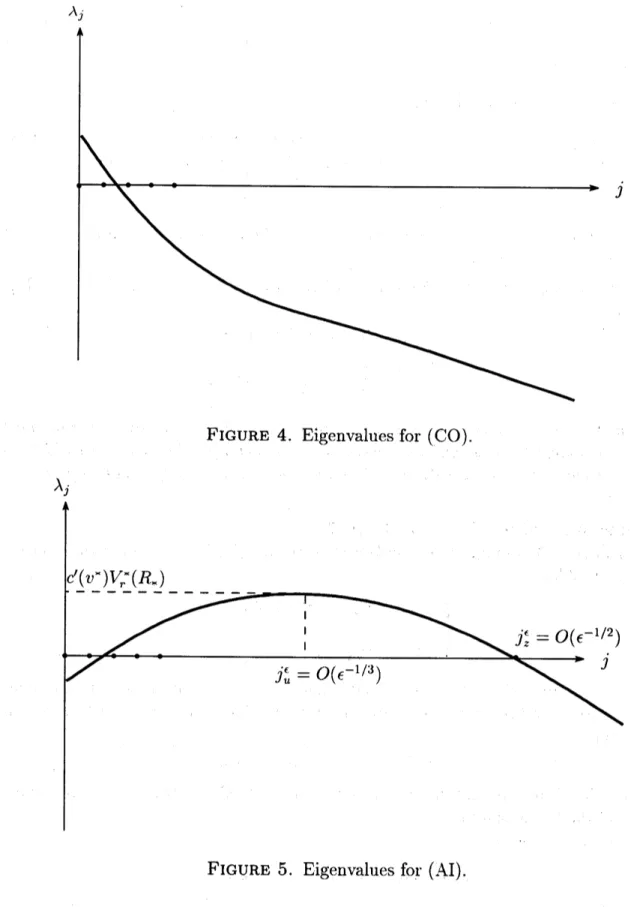
map $\Pi_{0}$.

Theorem 6([11]). The equilibrium solutions $(u^{\epsilon}(|x|), v^{\epsilon}(|x|))$

of

Theorem 5are unstable

with respect to (1.3). Moreover, there are (cf. Figures

_4and

5)

$\bullet$ two unstable eigenvalues _{$\lambda_{0}>\lambda_{1}>0$}

for

$(CO)’ nonlinearity$; $\bullet$ many unstable eigenvalues

for

(AI)-nonlinearity,

$\lambda_{0}<\lambda_{1}<0<\lambda_{2},\cdots$

.

$\dot{\prime}\lambda_{j_{C}}$,

where $j_{\epsilon}=O(\epsilon^{-1/2})$.

(10)

$\lambda_{j}$

$j$

FIGURE 4. Eigenvalues for (CO).

FIGURE 5.

Eigenvalues for (AI). In the $above_{i}$ the multiplicity _{$m_{j}$}

of

the eigenvalue $\lambda_{j}$ is given by

$,n_{j}= \frac{(2j+\grave{\wedge}-\prime 2\prime)(j+\sim^{l}\backslash ^{r}-3)!}{j!(\wedge\prime\backslash -2)!}$

.

(11)

which is the dimension

_of

the space

_of

spherical har monics

_of

degree$\ovalbox{\tt\small REJECT}$. Moreover,

eigen-function

associatedwith$\mathrm{A}_{\ovalbox{\tt\small REJECT}}$ are

of

the

form

$p(|\mathrm{r}|)\mathrm{O}(y)with|y|\ovalbox{\tt\small REJECT}$ ) and

0

being

a

spherical

harmonics

_of

degree$\ovalbox{\tt\small REJECT}\ovalbox{\tt\small REJECT}$.

We

now

state abifurcation result.

Theorem 7([11]). Assume that

$N=2$

and the

nonlinearity in (2.1)

is

_of

(AI)-type.

There eists a sequence $\{\epsilon_{j}\}$

for

sufficiently large $j$, say$j\geq O(\epsilon_{0}^{-1/2})$, with

$\epsilon_{j-1}>\epsilon_{j}arrow 0$ (as $jarrow\infty$)

such that when $\epsilon$ passes

$\epsilon_{j}$,

a non-radial

solution

$(u^{\epsilon,j}, v^{\epsilon,j})$

of

(2.1)

bifurcates from

the

trivial branch $(u^{\epsilon_{!}}.v^{\epsilon})$. Moreover,

(1) the symmetry group

_of

the

_bifurcated

solution $(u^{\epsilon,j}., v^{\epsilon,j})$ is the dihedral group $\mathrm{D}_{j}$

of

order$2j$

:

(2) the

_bifurcation

points $\epsilon_{j}$

are

explicitly characterized as:

$\epsilon_{j}=c’(v^{\mathrm{x}})\frac{W}{dr}.(R_{\mathrm{x}})\frac{1}{j^{2}}+O(\frac{1}{j^{4}})$ (as $jarrow\propto$).

Remark 2. The restriction $N=2$ in Theorem 7is only

_for

the sake

_of

avoiding the

algebraic complication in identifying subgroups

of

the orthogonal group $O(N)$ which have

$a$ one-dimension$al$

fied

point subspace.

Similar

results hold

for

$N\geq 3$ with

more

intricate

statements.

Outline of proof of Theorems 6and 7.

We linearize (1.3) around the trivial branch$(u^{\epsilon}(|x|)\dot, v^{\epsilon}(|x|))$ and consider the associated

eigenvalue problem:

(3.1) $\{\begin{array}{l}\epsilon\lambda\phi=\epsilon^{2}\Delta\phi+f_{u}^{\epsilon}\phi+f_{v}^{\epsilon}\psi\epsilon\lambda\psi=D\Delta\psi+g_{v}^{\epsilon}\psi+g_{u}^{\epsilon}\phi_{\dot{r}}\end{array}$

where $f_{u}^{\epsilon}$ etc. are

evaluated

at the trivial branch. The eigenvalues of (3.1)

are

divided

into two classes, critical and

non-critical

eigenvalues. An eigenvalue $\lambda^{\epsilon}$ of (3.1) is called

non-critical if

${\rm Re}\lambda^{\epsilon}arrow-\propto$ (as $\epsilonarrow 0$).

From this definition,

_we

_only need to examine the critical eigenvalues to determine the

stability ofthe trivial solutions $(u^{\epsilon}., v^{\epsilon})$.

The key is the following:

{critical

eigenvalues

of (3.1)} $\approx\sigma(A$‘).

Namely, the critical eigenvalues

are

well approximated by the eigenvalues of the operator

$A^{\epsilon}$. In

our

radially symmetric case, the eigenvalues of$A^{\epsilon}$ are explicitly given by

(3.2) $\lambda_{j}=c’(\iota^{\mathrm{x}}’.)[\frac{d\mathrm{L}^{r}/}{dr}.(R_{\mathrm{x}})-\frac{1}{D}\frac{[g]}{\gamma_{1j}}.]-\frac{\epsilon}{R^{2}}.(j-1)(j-1+-\nwarrow^{\vee})$ $(j=1.2.. )’\ldots$

(12)

$\frac{-1}{R_{\mathrm{x}}^{2}}(j-1)(j-1+N)$

is the $j$-th eigenvalue of the Jacobi operator

$\triangle^{\Gamma_{0}}+\sum_{k=1}^{\mathit{1}\backslash ^{r}-1}\kappa(x)^{2}$

on

$\Gamma_{0}=\{x\in \mathbb{R}^{N}||x|=R_{\star}\}$.

Let

us

recall here that $\pi_{j}$ is the$j$-th eigenvalue of the Dirichlet-t0-Neumann map

$\Pi_{0}$, and

it is asymptotically

characterized

([10])

as

(3.3) $\lim_{jarrow\infty}\frac{\pi_{j}}{\sqrt{j(j+l\mathrm{V}-2)}}=\frac{2}{R_{*}}$.

Moreover thanks to the maximum principle ([10]), one

can

prove that

(3.4) $\frac{dV^{*}}{dr}(R_{*})-\frac{1}{D}\frac{[g^{*}]}{-\pi_{j}}\{$

.

$<0$ if _$j=1,2$ $>0$ if $j\geq 3$.

From (3.2), (3.3) and (3.4), the statements in Theorem 6follows immediately.

The proof of Theorem 7is furnished by the equivariant branching lemma due to

Van-derbauwhede [12] and Cicogna [2], The characterization of the critical eigenvalues as in

(3.2)-(3.4) plays adecisive role in verifying the conditions of the branching lemma.

Acknowldgement: Over the last decase and ahalf, Ihave benefitted from so many

people, some directly and others indirectly through research papers,

on

the contents of

this article. Ilist names of these people to acknowledge their contributions. They are, in

alphabetical order: N. Alikakos, P. Bates, $\mathrm{X}$-F. Chen, $\mathrm{X}$-Y. Chen, M. del Pino, S.-I. Ei,

P. Fife, H. Fujii, G. Fusco, J. Hale, Y. Hosonl,$0.$_, H. Ikeda, M. Ito, $\mathrm{C}’$. Jones, X.-B. $\mathrm{L}i\mathrm{n}$, J.

Mallet-Paret, M. Mimura, N. Nefedov, Y. Nishiura, H. Suzuki, M. Tabata, I. Takagi, M.

Taniguchi, E. Yanagida, and many others.

REFERENCES

[1] X. Chen, Generation and propagation _{of interfaces}in

_{reaction-diffusion}

systems,Trans. Amer. Math. Soc, 334(1992), 877-913. $|$

[2] G.Cicogna, Symmetry Breakdown_from _Bifurcation. Lettere al Nuovo Cimento 31 (1981), 600-602.

[3] E. Conway, D. Hoff and J. Smoller, Large time behavior _ofsolutions _ofsystems _ofnonlinear

reaction-diffusion equations, SIAM J. Appl. Math. 35(1976), 1-16.

[4] P.C. Fife, Propagator-controller systems and chemicalpatterns, in: Non-Equilibrium Dynamics in Chemical Systems, eds. C. Vidal and A. Pacault (Springer-Verlag, Berlin 1984)$\dot{\prime}76- 88$.

[5] H. Ikeda. On the $asym,pto\dagger,ic$ solutions for a weakly coupled elliptic boundary value problem with $a$

small parameter, HiroshimaMath. J. 16(1986), 227-250.

[6] M. Mimura. M. Tabata and Y. Hosono, Multiple solutions oftwO-point boundary value problems _of

Neumunn type wr,th, _a sm,all_parameter, _{SIAM J.} _Math. Anal., _11(1980), _613-631.

[7] J.D. Murray, Mathematical Biology; Biomathematics Texts Vol. 19, _{Springer-Verlag Berlin}

Heidel-berg (1989).

[8] Y. Nishiura, Coexistence

_of

infintely many stable solutions to reaction

_diffusion

systems in the sin-gular $\lim,it$. Dynamics Reported. $3(1994)$

.

25-103

(13)

[9] Y. Nishiura and H. Fujii. Stability _ofsingularly perturbed solutions to systems _of_{reaction-diffusion}

equations. SIAM J. Math. Anal. 18(1987), 1726-1770.

[10] K. Sakamoto, Internal layers in high-dimensional domains. Proc. Royal Soc. of Edinburgh

$128\mathrm{A}(1998)$, 359-401.

[11] K. Sakamoto, Infinitely many_finemodesbifurcating

_from

radiallysymmetricinternal layers. Preprint (2000).

[12] A. Vanderbauwhede, Local Bifurcationand Symmetry. ${\rm Res}$. Notes Math. 75. Pitman, Boston,1982