Neuralnet Collocation Method for Solving Differential Equations (Computation mechanics and domain decomposition methods)

Neuralnet Collocation Method for Solving Differential

Equations

TatsuokiTAKEDA,Makoto FUKUHARA,Ali LIAQAT

Department of Information Mathematics and ComputerScience

TheUniversity of Electro-Communications

電気通信大学 竹田辰興、 福原誠、 リアカト・アリ

Abstract

Collocation method for solvingdifferential equations by using a

multi-layer neural network is described. Possible applications of the method are

investigated by considering the distinctive features of the method. Data

assimillationis one ofpromising applicationfields of this method.

1. Introduction

1.1 Neural network

In this article we present an application of afeed-forward multi-layer

neural network (neuralnet) as a solution method of a differential equation.

The feed-forward multi-layer neural network is a system composed of (1)

simple

processor

units (PUs) _{placed in layers and} (2) connections between

the PUs of adjacent layers (Fig.1). Data _{flow from the input} layer to the

output layer through the hidden (intermediate) _layers and the connections

to which weightsdeterminedbya training

process

are assigned. At each PU

of the hidden layers and the output layer weighted sum of the incoming

datais calculated and the result is nonlinearlytransformed by an activ ation

function and transferred to the next layer. Usually

some

kind of sigmoid

functions is used as the activation function. But at the output layer often

the nonlinear transformation is omitted. The neural network is usually

trained as follows. (1) A lot of datasets composed of input data and

corresponding output data (supervisor data) _{are prepared.} (2) _{Output data}

are calculatedby entering the input data to the input PUs accordingto the

above data flow. (3) _Sum of squared errors of the output data from the supervisor data is calculated. (4) $\mathrm{W}$eights assigned to the connections are

adjusted so that the above squared

sum

is minimized. The most

commonly used algorithm to this

process

is the gradient method and, in

propagation method based on the gradient method is implemented efficiently.

Fig.1 A schematicdiagramof a three-layeredneural network

1.2 Features ofaneural network

The feed-forward multi-layer neural network is characterized by

keywords of training, $\mathrm{m}$apping, smoothing, and interpolation. In relation

with the keywords, wemake use ofthe following distinctive features of the

neural network forour

purpose.

(1) Training$\cdot$

.

Optimization of the set of the weights with respect to an

appropriate object function is carried out. The object function of the

neuralnetwork isrepresented as

$E= \sum_{\mathrm{t}l^{nt}em}F(\vec{f}(\vec{x}_{t},\vec{p}n\ell em’)\mathrm{I}$

where $\vec{x}_{\mu \mathrm{f}tem}$ is

an

input data vector for the trainin$\mathrm{g}$ and

$\vec{p}$ is a vector representing the weights. For the feed-forward multi-layer neural

network the following type of object functionsisusually employed.

$\mathrm{p}(\vec{f}(_{\vec{X}_{\}nttem}}’\vec{\mathcal{P}}))=[\vec{f}(\vec{X}\vec{p}\mu ttem’)-\vec{f}_{\mu t}tem]\wedge 2$

Usually a sum of squared errors of output data from the prepared

remarked that there are other possibilities for choice of the object function. The training by the error back propagation method is

carried out as

$\vec{p}\Rightarrow\vec{p}-\alpha^{\frac{\partial E}{\phi^{arrow}}}$

(2) $\mathrm{M}\mathrm{a}_{\mathrm{P}\mathrm{P}^{\mathrm{i}\mathrm{g}}}\mathrm{n}\cdot$

.

By the neural network mappingfrom the input

space

to the

output

space

good approximation can be attained in$\mathrm{c}o$mparison with a

usualorthogonalfunction expansion. Itisbecause in this methodnot

only _{expansion coefficients but also the basis functions of the}

expansion themselves are optimized.

(3) _{Smoothingand interpolation: These are carried out in the meaning of}

theleast

square

fitting. It isimportant that these are always associated with the above neural networkmapping

processes.

1.3 Object function and aimsofour study

In _{our study we applied the feed-forward multi-layer neural network}

to the _{solution method of differential equations. Milligen et al., and}

Lagaris et al., _{have proposed} the method and demonstrated successful

results bythe method $[1,2]$

.

This is a kind of the collocation _{methods, i.e.,}

the wholeprocedureis describedasfollows.

(1) From the computational domain $\Omega$ a subdomain $\hat{\Omega}$

composed of

collocation points is constructed.

(2) _{The coordinates} of _{a collocation point are regarded as a pattern for the}

input dataof the neural network anda solution value correspondingto the coordinates isregarded asthe output dataofthe neural network.

(3) _{The residual of the differential equation is calculated from the output}

data and the squared residual is used as the object function. In this

process

it should be noted that the residual is expressed malytically

because the output data are the analytical functions of the input

variables with the weightvariables as parameters.

Difference of the methods by Milligen etal., _{and Lagaris} etal., is in the

treatmentof the $\mathrm{b}\mathrm{o}\mathrm{u}\mathrm{n}\mathrm{d}\mathrm{a}\mathrm{r}\mathrm{y}/\mathrm{i}\mathrm{n}\mathrm{i}\mathrm{t}\mathrm{i}\mathrm{a}\mathrm{l}$conditions. In the method$\mathrm{b}\mathrm{y}\overline{\mathrm{M}}\mathrm{i}\mathrm{l}\mathrm{l}\mathrm{i}\mathrm{g}\mathrm{e}\mathrm{n}$et

al., these conditions are treated as penalty terms in the object functions. These conditions are, therefore, satisfied only approximately. In the

method by Lagaris et al.,

on

the other hand, these conditions are exactly

network output variables. However, it is rather difficult

or

impossible to

find form factors appropriatefor a given problem.

Moreover, the solution method by using the neural network is

generally time-consuming in comparison with the well-studied

conventional solution methods of differential equati$o\mathrm{n}\mathrm{s}$ and it does not

seem useful to apply the neural network solution method to a usual

problemforsolving differentialequations.

Ouraims of the studyare describedasfollows.

(1) Extensionof themethod by Lagaris et al., to a method with

subdomain-defined form factors: As it is difficult to find a single appropriate form

factor which describesthe whole $\mathrm{b}\mathrm{o}\mathrm{u}\mathrm{n}\mathrm{d}\mathrm{a}\mathrm{r}\mathrm{y}/\mathrm{i}\mathrm{n}\mathrm{i}\mathrm{t}\mathrm{i}\mathrm{a}\mathrm{l}$conditions we divide

the domain into anumber of subdom ains and construct a set of a form

factor in each subdomain. We apply the method to a simple model

problem.

(2) Application of the neural network collocation method for data

assimilation problems: One of the distinctive features of the neural

network differential equation solver is that a smooth solution can be obtained even if $\mathrm{e}\mathrm{x}\mathrm{p}\mathrm{e}\mathrm{r}\mathrm{i}\mathrm{m}\mathrm{e}\mathrm{t}\mathrm{a}\mathrm{l}/\mathrm{o}\mathrm{b}\mathrm{s}\mathrm{e}\mathrm{r}\mathrm{v}\mathrm{a}\mathrm{t}\mathrm{i}\mathrm{o}\mathrm{n}\mathrm{a}\mathrm{l}$ noise is induded in

constraining conditions such as $\mathrm{i}\mathrm{n}\mathrm{i}\mathrm{t}\mathrm{i}\mathrm{a}\mathrm{l}/\mathrm{b}\mathrm{o}\mathrm{u}\mathrm{n}\mathrm{d}\mathrm{a}\mathrm{r}\mathrm{y}$conditions and so on.

By making use of this feature the method can be applied efficiently to

the data assimilation. We study basic problems concerning this

application.

2. Neuralnet collocation method(NCM)

2.1 Analytical expressionofderivatives of solution

In this subsection we consider a three-layered neural network. The

result can be extended easily to a network with more layers. An analytical

expression ofasolution isgiven as

$y_{k}= \sum_{j=1}^{f}w^{(}kj(_{\mathrm{i}=}2)\sum wX\sigma I1j(1i)i+w^{(}j01)1$

where $\mathrm{x},$ $\mathrm{y},$ $\mathrm{w}$, and $\sigma$ are the input variable, the output variable, the weight

variable, and the activation function (usually a sigmoid function: $\sigma(\mathrm{x})=$

$1/(1+\mathrm{e}^{\mathrm{X}})-)$,respectively.

$\mathrm{w}_{\mathrm{i}^{0}}$is the offset.

By differentiating the solution with respect to the input variables a

$\frac{\phi_{k}}{\partial\kappa_{\ell}}=\sum_{-,j1}^{j}w_{kj}^{(2}w_{j\ell}-)(1)\sigma 1(_{i-}\sum_{- 1}^{I}w_{ji}^{()}1xi^{+w^{(1})}j0)$

$\frac{\partial_{\mathcal{Y}_{k}}^{2}}{\partial\kappa_{\ell}\ _{m}}=\sum_{j--1}wwjkjj\ell(2)(1)w^{(1)}jm0\mathrm{J}(_{i}\sum_{=1}w^{(}Xw_{j0}^{(1)}Ijii^{+}1))$

where $\sigma^{\mathrm{t}}=d\sigma(\mathrm{x})/d\mathrm{X}$

.

By using these expression the residual of the $\mathrm{d}$

ifferential equation is expressed analytically. 2.2 Collocation method

We considerthe following differential equation.

$D^{arrow}\mathrm{y}=\vec{g}(_{\vec{X})},$ $\vec{x}\in\Omega$

where $\mathrm{D}$ is an operator. We assume the

output value of the neural

network is an approximation of the solution ofthedifferential equation, i.e.,

$\vec{y}\simeq\vec{f}(\vec{x},\vec{p}\rangle$

where $\vec{p}$ is the weights expressed

as

a

vector. The object function is,

therefore, expressedas

$\mathrm{E}=\int\{D\vec{f}(\vec{X},\vec{\mathcal{P}})-s^{(\vec{X}})\}^{2}d_{\vec{X}}$

Then the computational domain $\Omega$ is discretized to a domain $\hat{\Omega}$

of the collocation points and the object function for the collocation method is obtained as

$E= \sum_{pat\mathrm{f}e\Gamma n}F(\vec{f}(\vec{\chi}’\vec{p}pat\prime ern))$

$F(\vec{f}(\vec{x}_{p}\vec{p}at\prime ern’)\rangle=\{D\vec{f}(\vec{X}\vec{p}paftern’)-\vec{g}(X_{p\mathrm{f}m})ate\}$

$\vec{x}_{p\prime}\in atten\hat{\Omega}\subset\Omega$

2.3 $\mathrm{I}\mathrm{n}\mathrm{i}\mathrm{t}\mathrm{i}\mathrm{a}\mathrm{l}/\mathrm{b}\mathrm{o}\mathrm{u}\mathrm{n}\mathrm{d}\mathrm{a}\mathrm{r}\mathrm{y}$conditions

The boundary conditions ofthe Dirichlet typeare given as follows.

$\vec{y}(\vec{x}_{b})=\vec{y}_{b}$, $\vec{x}_{b}\in\Gamma$

where $\Gamma$ is the boundary of the computational domain. Essentially the

same discussion holds for other kinds of boundary conditions. Initial

conditions arealso treatedsimilarly.

According to the Milligen’s method the $\mathrm{i}\mathrm{n}\mathrm{i}\mathrm{t}\mathrm{i}\mathrm{a}\mathrm{l}/\mathrm{b}\mathrm{o}\mathrm{u}\mathrm{n}\mathrm{d}\mathrm{a}\mathrm{r}\mathrm{y}$ conditions

areimposedby preparingthefollowing objectfunction.

$\hat{E}=E+w_{b}$

$E_{b}= \sum_{i}(\vec{y}(_{\vec{X}_{b\mathrm{t}})-_{\hat{\vec{\mathcal{Y}}}}}\wedge bi)^{2}$

conditionsare given shouldnot necessarilybeplaced on the

computational

boundary.

In the case of the Lagaris’ method the solution of the differential

equation is approximated as $f(\vec{x},\vec{p})$ byusing the output data of the neural

network $\vec{f_{NN}}(\vec{x},\vec{p})$ as

$\vec{f}(\vec{x},\vec{p})=\vec{A}(\vec{x})+\vec{H}(\vec{x},\vec{f}_{N}N(\vec{X},\vec{p}))$

$\vec{A}(\vec{x}_{b})=\vec{y}_{b}$

$\vec{H}(\vec{x}_{b},\vec{f}_{NN}(_{\vec{X}\vec{p})}b’)=0$

For the Dirichlet boundary conditions $\vec{H}(\vec{x}_{b},\vec{f}_{NN}(\vec{\chi}\vec{p}b’)\mathrm{I}$ is expressed

as

a

product of an $\mathrm{a}\mathrm{p}\mathrm{p}_{arrow}\mathrm{r}\mathrm{o}\mathrm{p}\dot{\mathrm{n}}\mathrm{a}\mathrm{t}\mathrm{e}\mathrm{l}\mathrm{y}$chosen form factor and the output data of the

neural network $f_{\mathrm{N}N}(\vec{x},\vec{p})$. In this case the form factor vanishes at the

boundary.

3. Boundary conditionassignmentby divided form factors

In this section we describe the method to applythe Lagaris’ method to

problems with a complicated boundary shape. This is realized by dividing

the whole computational domain into subdomains with simpler boundary

shapes. $\mathrm{W}\mathrm{e}$ solve the Poisson equation in a

square

domain and in a

T-shaped domain. The Lagaris’ method cannot be applied directly to the

problem in the$\mathrm{T}$-shapeddomain and we divide the$\mathrm{T}$-shapeddomain into 7

subdomains.

3.1 Method of

a

divided form factor

The conditions which the form factor $\mathrm{g}$ used for the Dirichlet type

boundary condition should satisfy are summarized as 1) it vanishes on the boundary,2) it ispositive (or $\mathrm{n}\mathrm{e}\mathrm{g}\mathrm{a}\mathrm{t}\mathrm{i}\mathrm{v}\mathrm{e}$)

$- \mathrm{d}\mathrm{e}\mathrm{f}\mathrm{i}\mathrm{n}\mathrm{i}\mathrm{t}\mathrm{e}$in the domain, 3) it should

be sufficiently smooth, and 4) derivatives are easy to calculate. As far as these conditions are satisfied choice of the form factor is arbitrary. In the

followingwe considertwo examples,i.e., the case of the

square

dom ain and

the caseof the$\mathrm{T}$-shapeddomain.

(1) Example 1 (the

square

domain: $(-1,1)\cross(-\mathrm{L}1)$) (Fig.2)

Inthis casethe simplestform factoris expressedas

$x$

Fig.2 The

square

domain. $\mathrm{F}\mathrm{l}\mathrm{g}.3$ lhe 1-shapeddomain.

(2)_{Example 2} (the$\mathrm{T}$-shaped domain:$(-1,1)\cross(0,1)\cup(-1/2,1/2)\cross(-1,1)$)

(Fig.3)

Forthis case an exampleofthe divided form factorisgiven as

$g(X,\nu^{)}=\{$ $x(1+x)\mathrm{y}(1-y)$ $(\overline{\Omega}_{1})$ $x(1-x)y(1-y)$ $(\overline{\Omega}_{2})$ $y(1-y)/4$ $(\overline{\Omega}_{3}\rangle$ $(1/4-x)2(1-\mathrm{y})2/4$ $(\overline{\Omega}_{4})$ $r_{1}(1-r_{1})/4$ $(\overline{\Omega}_{5})$ $r_{1}(1-\gamma)1/4$ $(\overline{\Omega}_{\text{\’{o}}})$ 1/16 $(\overline{\Omega}_{7})$ $(_{r_{2}\sqrt{(_{X}-1/2)^{2}+\nu^{2}}}^{r_{1}}=\sqrt{(_{X}+1/2)^{2}+y2})=$ (_$g:C^{1}$ class) 3.2 Model problems

As amodel equation

we

consider the followingPoissonequation,

$\Delta u=-(20X-3\frac{15}{2}\chi\lambda y-3\nu)-6(X^{5}-\frac{5}{4}X^{3}+\frac{1}{4}\chi\psi$ in $\Omega$

$u=0$ on $\Gamma$

XVe solve the above equation for the two types of computational domains

(Fig.4) describedin theprevioussection. The exactsolution isgiven for the

aboveproblems as

Fig.4The computationaldomains for the modelproblems.

For simplicity ofprograming

we

employed

a

training algorithm composed of

a random search and the linear least square method instead of the

conventionaly used

error

backpropagation method. The structure of the

neural network is composed of two PUs in the input layer, 40 PUs in the

$\mathrm{l}\dot{\mathrm{u}}\mathrm{d}\mathrm{d}\mathrm{e}\mathrm{n}$layer, and 1 PU in theoutput layer(we denote this structure

as

2-40-1). Theresults ofthe calculations areshownin Figs.5-8 and the magnitude

of the errors is summarized in Table 1, where the maximum random value

denotes the maximum range ofthe initially assigned weights.

(a) (a)

(b) $(\mathrm{b}\rangle$

(c) (c)

Fig.5 Birdeyeviewof the solution Fig.6Birdeye view ofthe solution

inthe

square

domain in$\mathrm{T}$-shaped domain

(a)NN collocation, (b) exact, (a)NN collocation, (b) exact.

Numerical solution

(a) (b)

Fig.7 Contourplot of the solution (a)_{in the}

square

_{domain and}the

corresponding error.

Numericalsolution Absoluteerror

(a) (b)

Fig.8 Contour plotof the solution (a) in the$\mathrm{T}$-shaped domain andthe

corresponding error.

4. ApplicationofNCM to a dataassimilation problem

In this chapter we study basic issues of the neuralnet collocation

method relatingto the data assimilationproblems. 4.1 Irregular$\mathrm{b}\mathrm{o}\mathrm{u}\mathrm{n}\mathrm{d}\mathrm{a}\mathrm{r}\mathrm{y}/\mathrm{i}\mathrm{n}\mathrm{i}\mathrm{t}\mathrm{i}\mathrm{a}\mathrm{l}$conditions

In order to investigate the possibilityto applythe neuralnet collocation

method to the data assimilation problem we solve differential equations

4.2 Solution of Lorenz equation

In this section we solve the Lorenz equation by assigning initial

conditionsat different_{temporal points,} $\mathrm{t}_{0\cross},$

toY’

md $\mathrm{t}_{0\mathrm{Z}}$ forthree variables, X, $\mathrm{Y}$, and $\mathrm{Z}$, respectively. For training the network we employed a

combination of the error back-propagation method and the quasi-N$e$wton

method. The Lorenz equationis

$\frac{dX}{dt}=\sigma(Y-\mathrm{x})$

$\frac{dY}{dt}=r\mathrm{X}-\gamma-\mathrm{X}\mathrm{Z}$

$\frac{dZ}{dt}=\mathrm{X}Y-b\mathrm{z}$

$X(t_{0\mathrm{X}})=\mathrm{x}_{0},$ $Y(t_{0Y})=Y_{0},$$Z(t_{0\mathrm{z}^{)}}=Z_{0}$

Theobjectfunctionof the neuralnet collocation methodis given

as

follows.

$E= \sum_{t\in\hat{D}}\wedge\lfloor_{- t}\wedge$

$\hat{D}\subset Dand|\hat{D}|<\infty$

$X_{t}=A+(t-t_{0\mathrm{x}})f_{\mathrm{N}}N(\mathrm{f},\vec{p}_{\mathrm{X}})$

$Y_{t}=B+(t-t_{0)}’)f_{N}N(t,\vec{\mathcal{P}}\gamma)$

$Z_{t}=C+(t-\mathrm{f}_{0\mathrm{Z}})f_{NN}(t,\vec{\mathcal{P}}\mathrm{z})$

$t\in D,$ $D=[0,0.4]$, $A=x(t_{\mathrm{o}\mathrm{x}}),$ $B=\mathrm{Y}(to\mathrm{Y}),$ $C=Z(t_{0})\mathrm{z}$

At first, above equation is solved by the Runge-Kutta method for the

following conditions to obtain

a

base solution for comparison of the neuralnet collocation method.

$t\in D=[0,0.4]$

$X_{0}=0.0,$ $Y_{0}=1.0,$ $Z_{0}=0.0$, $t_{0\mathrm{X}}=t_{0\mathrm{Y}}=\mathrm{f}_{0Z}=t_{0}=0,0$ $\sigma=1.0,$ $r=28.0,b=8/3$

Next, we solve the same problem by the neuralnet collocation method

imposing the initial condition at $\mathrm{t}=0$

.

The results by the Runge-Kutta

method and the neuralnet collocation method

are

shown in Fig.9, where

they are indistinguishable each other in this scale. The error of the results

quasi-Newtonprocedure.

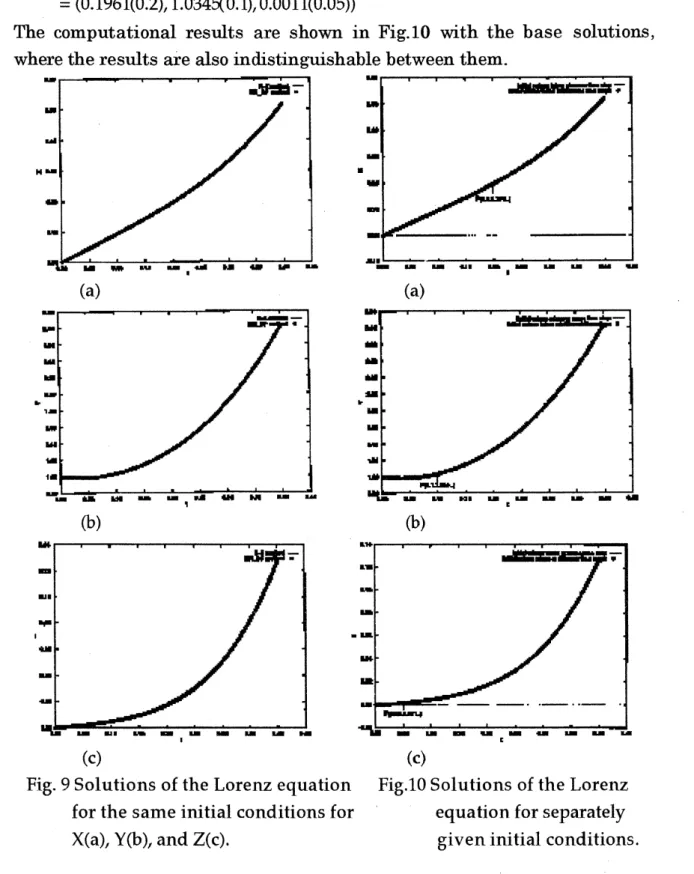
Then we solved the Lorenz equation for initial conditions imposed

separately to different variables, X, $\mathrm{Y}$, and Z. The initial conditions were

obtained from thebasesolutionbythe Runge-Kutta method as

$(X_{0}(t_{0\mathrm{X}}),Y_{0}(t_{0\mathrm{Y}}),Z0(t_{0\mathrm{z}}))$

$=(0.1961(0.2),1.0348^{0}\cdot 1),0.0011(0.05))$

The $\mathrm{c}\mathrm{o}\mathrm{m}\mathrm{D}\mathrm{u}\mathrm{t}\mathrm{a}\mathrm{t}\mathrm{i}_{\mathrm{o}\mathrm{n}}\mathrm{a}1$ results are shown in $\mathrm{F}\mathrm{i}\epsilon.10$ with the base solutions,

la) $\iota \mathrm{a}|$

1D1 (Dl

(C) (c)

Fig. 9 Solutions of the Lorenz equation Fig.10 Solutions ofthe Lorenz

for the sameinitial conditions for equationfor separately

4.3 Solutionof

a

heatequation

In order to _{investigate a possibility}to apply the neuralnet collocation method to the data assimilation problem we consider to solve the heat equation forirregularly imposedinitial conditions.

$\alpha^{2}\frac{\partial^{2}u}{h^{2}}+\sin 3m-\frac{\partial u}{\partial t}=0$, _{$(x,t)\in D=[0,1]\cross[0.1]$}

$\alpha=1$

$u(\mathrm{O},t)=u(1,t)=0.\mathrm{O}$

$u(x, 0)=\sin\pi x$

The analytical _{solution to the above}problem is given as

$u(x,t)= \exp(-(m)2t)\sin\pi X+\frac{1-\mathrm{e}\mathrm{x}_{\mathrm{P}}(-(3m)2t)}{(3\pi\alpha)^{2}}\sin 3\pi x$

The

same

problem

was

solved by the neuralnet $\mathrm{c}\mathrm{o}\mathbb{I}_{0}\mathrm{c}\mathrm{a}\mathrm{t}\mathrm{i}_{\mathrm{o}\mathrm{n}}$method. The

result is shown with the analytical solution in Fig. 11. Results with the

average

errors

of3.49E-3 and 1.33E-3 are obtained after 20000 iteration of

the ba&-propagationmethod, and5 iterations of the quasi-Newton method,

respectively. By _{giving initial conditions for} $\mathrm{i}\mathrm{r}\mathrm{r}\mathrm{e}\omega \mathrm{a}\mathrm{r}\mathrm{l}\mathrm{y}$ placed spatial

points _{almost similar results}

_were

_obtained.

晶億億$\mathrm{m}\iota \mathrm{K}$

.

h’–輸 d –

$\blacksquare$

5. Discussionandconclusion

for the$\mathrm{i}\mathrm{n}\mathrm{i}\mathrm{t}\mathrm{i}\mathrm{a}\mathrm{l}/\mathrm{b}\mathrm{o}\mathrm{u}\mathrm{n}\mathrm{d}\mathrm{a}\mathrm{r}\mathrm{y}$conditionsis successfully appliedto solution of

Poisson equation in a

square

domain and in a $\mathrm{T}$-shaped domain. To

attainhigher accuracy some improvements arenecessary.

(2) In order to study apoSsibilit‘yto applythe neuralnet collocation method

for the data assimilation problem simple model problems on the

Lorentz equation and the heat equation

were

solved. Promising

resultswere obtained.

References

[1] B.Ph. vanMilligen, et al.,_Phys. Rev. Letters75 (1995) 3594-3597.