Economic Growth?
journal or
publication title
The B.E. Journal of Macroeconomics
volume
6
number
1
page range
1-30
year
2006
Contributions to Macroeconomics
Volume 6, Issue 1 2006 Article 5
What Does the Solow Model Tell Us about
Economic Growth?
Toshihiro Okada
∗∗School of Economics, Kwansei Gakuin University, [email protected]
Economic Growth?
∗
Toshihiro OkadaAbstract
This paper presents, within a framework of the Solow model, evidence that there are sig-nificant differences in convergence patterns across subsamples. It shows that although OECD countries and the countries converging to their steady states from above follow a pattern of con-ditional convergence, those converging to their steady states from below do not. This result is best explained by the idea that technology diffusion has a large effect mainly on the countries converging to their steady states from below.
KEYWORDS: convergence, Solow model, technology diffusion
∗I would like to thank Antonio Ciccone, Charles I. Jones (the editor), Xavier Sala-i-Martin,
Jonathan Temple, Gylfi Zoega and anonymous referees for their helpful suggestions. I also benefited from the comments of Reza Arabsheibani, Andrew Mountford, Michael Spagat, Jonathan Wadsworth, participants at Royal Holloway Economic Workshop and Young Economist Conference in the University of Oxford. All remaining errors are mine. Toshihiro Okada, School of Economics, Kwansei Gakuin University, 1-155 Uegahara Ichiban-cho, Nishinomiya, Hyogo 662-8501 Japan. Tel.+81-(0)798-54-6496. Fax.+81-(0)798-51-0944. E-mail: [email protected]
There has been controversy over the growth regressions deployed in neoclas-sical growth models. This is generally referred to as the ‘convergence contro-versy’. The neoclassical growth models suggest that an economy converges to its own steady state. This implies that if we control for the exogenously determined variables such as the population growth rate and the investment rates of physical and human capital, and assume that all of the economies face the same exogenously determined constant growth rate of technology, we should observe that the country with the lower initial output per capita tends to grow faster: conditional convergence. Mankiw, Romer, and Weil (1992) (henceforth, MRW) undertake a cross-country regression analysis and find evidence for conditional convergence by augmenting the Solow model with human capital. Barro and Sala-i-Martin (1992a, 1992b) carry out convergence tests by using regional data on Japan and the US, and observe convergence within these two countries. MRW (1992), and Barro and Sala-i-Martin (1992a, 1992b) both conclude that the estimated speed of convergence, β , is about 0.02 per year around the steady state. This implies a relatively slow speed of
convergence: an economy moves halfway to its steady state in about 35 years.1
Despite these findings, many economists criticize the neoclassical growth models and their empirical tests. Romer (1990), Grossman and Helpman (1991), and Aghion and Howitt (1992) are not satisfied with the assump-tion of exogenous technological change and establish models that endogenize technological progress. Most important, many researchers argue that the idea of treating technology as a nonrival and non-excludable good in the
neoclas-sical growth models is not appropriate.2 They argue that it is indefensible
to assume a common growth rate of technology and a common initial level of technology in the cross-country regressions. The levels and growth rates of technology somehow should differ across countries.
This paper attempts to show what the conventional analysis of the Solow model tends to miss out, and reconsiders the validity of the model by applying a new cross-country regression method. We allow initial levels and growth rates of technology to vary across countries. To perform the convergence tests, we use the method which not only directly controls for saving and population growth rates but also indirectly controls for initial levels of technology by using capital output ratios (It is, thus, different from panel data studies of growth convergence).
1Although the studies by Barro and Sala-i-Martin (1992a, 1992b) do not control for
steady state determinants, convergence is observed because the steady states are assumed to be similar across regions.
2Romer (1994) argues that important discoveries are usually excludable at least for some
The empirical results show significant differences in convergence patterns across subsamples. When the sample is divided into three subsamples: OECD countries (‘OECD’ sample), countries converging to their steady states from above (‘Above’ sample) and countries converging to their steady states from below (‘Below’ sample), conditional convergence is observed only in the ‘OECD’ and ‘Above’ samples. This result is best explained by the idea that technology diffusion has a large effect mainly on the countries converging to their steady states from below. The paper also shows that the estimated coefficient for the speed of convergence could be larger than the conventional estimated value without contradicting the Solow model’s prediction.
Section 1 re-examines the motion of an economy within the framework of the Solow model by using capital per labor rather than capital per effective labor. This approach allows us to analyze the effect of the initial level of technology on the motion of the economy. Section 2 describes the shortcomings of MRW’s cross-country regressions. Sections 3 and 4 show the empirical results. Section 5 discusses the implication of the results. Section 6 concludes.
1
Alternative Analysis of the Solow Model
A conventional approach to analyzing the motion of an economy in the Solow model is to use capital per effective labor. However, capital per labor is used throughout this paper. This approach allows us to pay greater attention to the level of technology in analyzing the model.
1.1
The Model
We consider a Cobb-Douglas production function case in the Solow (1956) model. It takes the form of labor-augmenting technological progress. The function at time t is, therefore, given by:
Y (t) = K(t)α(A(t)L(t))1−α 0 < α < 1, (1)
where Y , K, A and L denote output, capital, the level of technology and labor, respectively. The Solow model assumes that the growth rates of population and technology are exogenously determined. Thus, the level of technology and amount of labor at time t are given by:
L(t) = L(0)en t (2)
where L(0) and A(0) are the initial amount of labor and the initial level of technology, respectively. L and A grow at the exogenously determined rates
nand g.
Assuming that the rates of saving and depreciation are exogenous and constant, the evolution of capital can be described as:
·
K(t) = sY (t)− δK(t), (4)
where a dot over a variable, such as K(t), denotes differentiation with respect·
to time, and s and δ are the rates of saving and depreciation, respectively. By defining k(t) as capital per unit of labor, the evolution of k(t) is given by:
·
k(t) = sA(0)1−αe(1−α) g tk(t)α− (n + δ)k(t). (5)
Notice that equation (5) describes the evolution of K(t)/ L(t) but not the evolution of K(t)/(A(t)L(t)). This approach makes it possible to capture the impact of differences in the initial levels of technology A(0) on the levels and growth rates of income per unit of labor.
1.2
The Graphical Analysis of the Dynamics
In this sub-section we analyze the dynamics of the model by using a phase diagram. We draw the diagram in the (t, ln k) space. This seems odd at first since one of the variables is time t. This approach, however, works fine. The only difference from the conventional phase diagram analysis is that the direction of motion of t (one of the variables in the diagram) is exogenously given, that is, t rises regardless of the level of ln k.
To analyze the direction of motion of ln k, we first consider the case when dk(t)/dt = 0. By setting dk(t)/dt = 0, equation (5) gives:
ln k(t) = 1
1− αln s−
1
1− αln(n + δ) + ln A(0) + g t. (6)
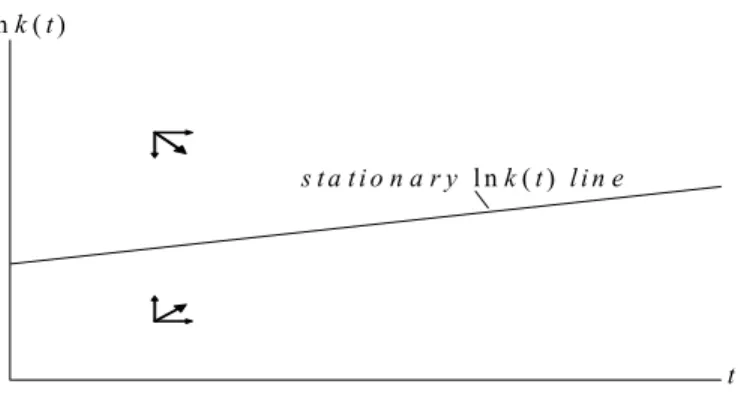
Equation (6) describes all combinations of t and ln k(t) which give zero growth rate of k(t). Since α , s, n, δ and g are constant, equation (6) is a linear line in the (t, ln k) space. The slope of the line is g. We call this line the ‘stationary ln k line’ (Figure 1 shows the line). It shows the collection of points in the
(t, ln k) space such that dk(t)/dt = 0 holds. In other words, the stationarity
is only local. Note that, the stationary ln k line does not at all characterize a steady state. It just provides us the dk(t)/dt = 0 locus in the (t, ln k) space
s t a t i o n a r y l n k ( t ) l i n e l n k ( t )
t
Figure 1: The dynamics of ln k(t) over time
and it divides the space into two regions. The direction of motion of ln k depends on whether ln k is below or above the stationary ln k line.
We can find out the direction of motion of ln k by considering two cases:
dk(t)/dt > 0 and dk(t)/dt < 0. When dk(t)/dt > 0, we get the following
expression from equation (5).
ln k(t) < 1
1− αln s−
1
1− αln(n + δ) + ln A(0) + g t. (7)
Equation (7) implies that the direction of motion of ln k at a given point of time t is upward (i.e., dk(t)/dt > 0) when ln k is below the stationary ln k line. Similarly, when dk(t)/dt < 0, we get the following expression from equation (5).
ln k(t) > 1
1− αln s−
1
1− αln(n + δ) + ln A(0) + g t. (8)
Equation (8) implies the direction of motion of ln k at a given point of time
t is downward (i.e., dk(t)/dt < 0) when ln k is above the stationary ln k line.
Thus, since t rises regardless of the level of ln k, the dynamics of ln k over time can be shown as in Figure 1. The figure shows that ln k falls over time when
ln kis above the stationary ln k line and rises over time when ln k is below the
stationary ln k line.
To see the dynamics of ln k(t) in more detail, we simulate the model by using the following equation: (solving the first-order differential equation (5)
20 40 60 80 100 1.5 2.5 3 3.5 l n k ( t ) t s t a t i o n a r y l n k ( t ) l i n e l n k * ( t ) l i n e
Figure 2: The stationary ln k(t) line and the steady state and taking logs yield the following equation)
ln k(t) = 1
1−αln[k(0)1−αe−(n+δ) (1−α)t(g + n + δ) + s A(0)1−α(eg (1−α)t− e−(n+δ) (1−α)t)]
−1−α1 ln(n + g + δ).
(9) To carry out simulations, we apply commonly used values for the parameters:
α = 0.33, g = 0.02, n = 0.015, δ = 0.05 and s = 0.21. Furthermore, at
this stage, we assume that the initial level of technology, A(0), is fixed at 1. For convenience, the initial levels of capital per unit of labor, k(0), are set between 0.01 and 50 (since the purpose of this analysis is to graphically capture the dynamics of k(t), the choices of k(0) and A(0) do not cause any serious problems in the analysis).
Figure 2 shows the movement of ln k(t) over time for various levels of ln k(0). Each curve represents the movement of ln k(t) over time for the corre-sponding ln k(0). The higher position of the curve implies the higher level of k(0). Figure 2 confirms the point made before. ln k(t) falls (rises) over time when ln k(t) is above (below) the stationary ln k line. On the stationary ln k line, the growth rate of k(t) is zero (i.e., the stationary ln k line intersects with ln k(t) curves at the bottom of ln k(t) curves). Figure 2 also shows that
ln k(t) converges to a line which is parallel to the stationary ln k line. We call
this line the ‘ln k∗ line’. It describes the steady state path of ln k(t). Since the
stationary ln k line is given by equation (6), the growth rate of k(t) on the
ln k∗ line is g. Therefore, k(t) converges to the steady state where the growth
rate of k(t) is g. The level of k(t) in the steady state is denoted as k∗(t). The
important fact here is that the position of the ln k∗ line depends on that of
ln k ( t) 20 40 60 80 100 3 4 5 6 t s ta tio n a r y ln k ( t) lin e 2 s ta tio n a r y ln k ( t) lin e 1 ln k ( t) c u r v e 2 ln k ( t) c u r v e 1
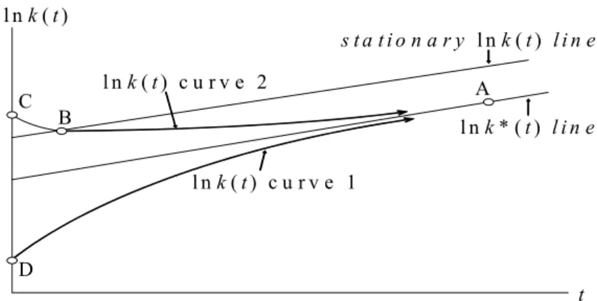
Figure 3: The impact of the difference in A(0)
of ln k(t). The higher position of the stationary ln k line leads to the higher position of the ln k∗ line.
We next analyze the impact of differences in initial levels of technology on the dynamics of k(t). ln k(t) curves are traced with two different levels of A(0), (A(0) = 1 and 11). The same values for s, α, n, g and δ are used as in the previous analysis, but k(0) is fixed at 15 this time.
Figure 3 shows the analysis. ln k(t) curves 1 and 2 correspond to the levels of A(0) of 1 and 11, respectively. Stationary ln k line 1 and 2 correspond to the levels of A(0) of 1 and 11, respectively. As in Figure 2, each ln k(t)
curve converges to its own ln k∗ line. The higher level of A(0) implies the
higher position of the stationary ln k line. Since the position of the ln k∗ line
depends on that of the stationary ln k line (which is described by equation
(6)), k∗(t) depends on α, n, δ, s, g and A(0). Thus, assuming α, δ and g are
the same across countries, not only s and n but also A(0) affect the steady state level of k(t) and the non-steady state growth rate of k(t).
Finally, we characterize three different kinds of paths towards the steady state. In Figure 4, ln k(t) curve 1 shows the dynamics of ln k(t) when ln k(0)
is less than ln k∗(0), and ln k(t) curve 2 shows the dynamics of ln k(t) when
ln k(0)is greater than ln k∗(0). The two curves converge to the same ln k∗ line
since we assume the same levels of A(0), s, n and δ. Points C and D show the
starting points for each curve. At point B, d ln k(t)d t = 0 . At around point A,
ln k(t)' ln k∗(t). Notice that there are three kinds of paths. Between point C
and point B (Path 1), ln k(t) decreases and the growth rate of k(t) increases. Between point B and point A (Path 2), ln k(t) and the growth rate of k(t)
A l n k * ( t ) l i n e s t a t i o n a r y l n k ( t ) l i n e l n k ( t ) c u r v e 1 l n k ( t ) c u r v e 2 t l n k ( t ) B C D
Figure 4: Three types of ln k(t) paths
both increase. Between point D and point A (Path 3), ln k(t) increase and the growth rate of k(t) decreases. The economies on Path 3 converge to their steady states from below and the economies on Path 1 and Path 2 converge to their steady states from above.
Cho and Graham (1996) test the Solow growth model and find that many countries (especially, poor ones) converge to their steady states from above. Thus, it might be useful to look at the more details of characteristics of Path 1 and Path 2. The economies on Path 1 run down their capital-labor ratios (and also their capital-effective labor ratios) over time. Contrarily, the capital-labor ratios of the economies on Path 2 increase at a lower rate than g to reach their steady states (but their capital-effective labor ratios decrease over time). The important point is that it is possible for countries to converge to their steady states from above by increasing their capital-labor ratios.
1.3
The Graphical Analysis of the Speed of
Conver-gence
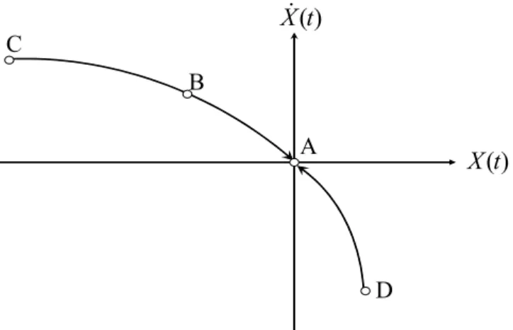
As Figures 2 and 3 show, an economy converges to its own steady state regard-less of where k and A start. We next consider the speed of convergence to the steady state. Corresponding to the analysis in Figure 4, Figure 5 shows the
dy-namics of an economy in the (d (ln k∗(t)− ln k(t)) /dt, ln k∗(t)− ln k(t)) space.
X and dX/dt denote ln k∗(t)−ln k(t) and d (ln k∗(t)− ln k(t)) /dt, respectively.
The speed of (conditional) convergence is defined as how rapidly the
B ) (t X& ) (t X C A D
Figure 5: The speed of convergence is thus given by:
β(t) =−
· X(t)
X(t). (10)
As we can see in Figure 5, if the economy starts below the steady state, the speed of convergence gets slower over time, but if the economy starts above the steady state, it gets faster over time. Figure 5 also shows that the absolute value of the slope of the curve can be a good approximation of β(t) around the steady state (i.e. around point A). Therefore, β(t) around the steady state can be given by:
β(t)' −d
· X(t)
d X(t). (11)
After some manipulation (see Appendix 1), equation (11) can be expressed as:
β(t)' −d · X(t) d X(t) = (1− α)(n + g + δ) µ y∗(t) y(t) ¶1−α α . (12)
Equation (12) shows that β(t) is (1 − α)(n + g + δ) when the economy is at the
steady state.3 Later in this paper, equation (12) will be used to derive a specific
equation to test the Solow model and to estimate the speed of convergence.
3The convergence rate when the economy is at the steady state is shown also by Barro
2
Growth Regression and the Initial Level of
Technology
The work of Mankiw, Romer and Weil (1992) shows that the augmented Solow model with human capital can explain a great deal of cross-country income differences without contradicting the model’s prediction and obtaining an un-realistic estimate for the elasticity of output with respect to (physical) capital. They also find evidence of conditional convergence. However, there exist some problems in their tests.
Their equations (without a role for human capital) are given by:
ln yi = a + α 1− αln si− α 1− αln(ni+ g + δ) + ²i (13) and ln³y(0)y(t)´ i = (1− e −β t)a + g t + (1− e−β t) α 1−α ln si −(1 − e−β t) α 1−αln(ni+ g + δ)− (1 − e−β t) ln y(0)i+ (1− e−β t)²i, (14)
where i indexes countries, yi is income per capita in 1985, ln(y(t)/y(0))i is log
difference of income per capita 1960-1985, ² is a country specific shock, and
a is a constant. The growth rate of technology, g, is assumed to be the same
across countries. Equation (13) is their estimated equation for the test of the steady state income per labor, and equation (14) is for the test of conditional convergence. The term, β, in equation (14) is the convergence coefficient which is obtained by use of a first-order approximation around the steady state, (i.e.
β = (1− α)(n + g + δ)). MRW get the implied β from the coefficient on
ln y(0) (thus, they restrict the values of β to be the same across countries to
get the generalized value of β). In setting these equations, they assume that
ln A(0)i = a + ²i. That is, they try to explain the variation in the initial level
of technology across countries by using the error term.
MRW assume that the country’s initial level of technology is not correlated with the regressors. That is, the error term, ², is assumed to be uncorrelated with independent variables. This is a very weak assumption particularly in equation (14). It is highly unlikely that there is no correlation between ² and ln y(0). In practice, the correlation between ² and ln y(0) seems likely to be
quite strong.4 Thus, the estimated coefficients will be seriously biased (MRW
mentioned about this problem in their article).
4Hall and Jones (1999) show that differences in the measured productivity levels across
In the following sections we attempt to estimate the Solow model by taking a different approach from MRW. We assume that technology is not a worldwide good but rather a domestic good. Thus, we allow for different initial levels and growth rates of technology across countries. We also assume that there
is no technology diffusion across countries.5 Thus, technology is completely
excludable across countries and differences in technology levels persist over time. Based upon these assumptions, we derive the estimated equation in which the impact of differences in unobservable initial levels of technology is incorporated without relying on the error term.
3
Empirical Test 1
3.1
The Specification
Our aim is to find a way to control for the unobservable initial levels of technol-ogy in the regression in order to test the Solow model. We derive our empirical specifications below.
From equations (1), (2), (3) and (4), the equation for the motion of K/AL can be expressed as:
·
bk(t) = sbk(t)α
− (n + g + δ)bk(t), (15)
where bk is K/AL, capital per effective labor. The standard approach to the
Solow model shows that dbk(t)/dt is equal to zero at the steady state. Thus
equation (15) can be rewritten as:
k∗(t) = s1−α1 (n + g + δ)1−1−αA(t) = s 1
1−α(n + g + δ)1−1−αA(0)eg t, (16)
where k∗(t) is the steady state level of capital per labor at time t. From
equation (1), the intensive form of the production function is given by:
y(t) = A(0)1−αe(1−α) g tk(t)α. (17)
Thus, the steady state level of output per labor is given by:
y∗(t) = A(0)1−αe(1−α) g tk∗(t)α. (18)
Substituting equation (16) into equation (18) yields:
y∗(t) = A(0)s1−αα (n + g + δ)1−α−αeg t. (19)
The initial level of output per capita is given by (from equation (17)):
y(0) = A(0)1−αk(0)α. (20)
Solving this expression with respect to A(0) yields: A(0) = µ k(0) y(0) ¶−α 1−α y(0). (21)
Substituting equation (21) into equation (19) and taking logs give: ln µ y∗(t) y(0) ¶ i − git =− α 1− αln µ k(0) y(0) ¶ i + α 1− αln si− α 1− αln(ni+ gi+ δ), (22) where i indexes countries and δ is assume to be constant across countries.
We assume
gi = g +egi,
where g represents the rate of technology growth which is constant across
countries and egi reflects deviations in technology growth from g. By use of a
first order Taylor-Series expansion of ln(ni+ gi+ δ)around gi = g, we get:
ln(ni+ gi+ δ)' ln(ni+ g + δ) + egi
(ni + g + δ)
. Substitution of this into equation (22) gives the following equation:
ln µ y∗(t) y(0) ¶ i −g t = − α 1− αln µ k(0) y(0) ¶ i + α 1− αln si− α 1− αln(ni+ g + δ) + ²i, (23) where ²i = µ t− α 1− α 1 (ni+ g + δ) ¶ egi. (24)
The restricted version of the equation is given by: ln µ y∗(t) y(0) ¶ i − g t = − α 1− α µ ln µ k(0) y(0) ¶ i − ln si + ln(ni+ g + δ) ¶ + ²i. (25) Equations (23) and (25) are the specifications used in this section. We
is random. It is also assumed that the countries are at their steady states at year t (or at least close to their steady state at year t so that most of variation
in ln(y∗(t)/y(t)) is due to country-specific demand shocks).
In our estimation, our main goal is not to uncover the true value of the capital share, α. Instead, we think we know that α is about 1/3. Hence, the estimation can help us to learn something about the nature of the error term.
Ifegi is independent with ln (k(0)/y(0))i, si and ni, and the countries are close
enough to their steady states at year t, we should be able to get the OLS estimator of α close to 1/3.
Another important point is the inclusion of the term ln (k(0)/y(0)) in equa-tion (23). Like convenequa-tional growth regressions, s and n enter in the regressions so that differences in the rates of saving and population growth are controlled
for. The term ln (k(0)/y(0)) is unusual one.6 By rewriting equation (21), one
can obtain: k(0) y(0) = µ A(0) y(0) ¶−1−α α .
Thus, the inclusion of ln (k(0)/y(0)) in equation (23) implicitly captures the negative correlation between the initial level of per capita output and the subsequent growth rate of per capita output if differences in initial levels of technology are controlled for. In short, the specification directly controls for the rates of saving and population growth and indirectly controls for initial
levels of technology.7
Our methodology is different from a panel data approach which treats the
initial level of technology A(0)i as a fixed effect. The panel data studies of
growth convergence include Islam (1995), Caselli, Esquivel and Lefort (1998), and Bond, Hoeffer and Temple (2001), among many others. The majority of the panel data studies allow only for different initial levels of technology but
do not allow for different growth rates of technology.8 However, our method
6Benhabib and Gali (1995) also use the capital-output ratio to control for the
unobserv-able initial levels of technology. In order to control for other determinants of the steady state, they treat them as fixed effects and difference them away by splitting the sample period. However, as Durlauf (1995) argues, this method is likely to reduce the power of the test relative to conventional tests, e.g., MRW (1992), because the null hypothesis is no conditional convergence and the conventional tests reject the null hypothesis by including a set of other control variables.
7We do not consider the role of human capital. Its omission is problematic and future
research should work to incorporate human capital into the framework.
8The studies by Lee, Pesaran and Smith (1997, 1998) are exceptions. They allow for
differences in the rates of technology growth. However, they do not report the implied values of α which can provide important information for testing the Solow model. Islam (2003) points out that the implied values of α are likely to be very low when worked out in
allows for differences in growth rates of technology as well as differences in initial levels of technology. Another advantage of our approach over the panel data approach is that it does not have a problem that would arise if one uses the panel data approach to control for initial levels of technology. As argued by many authors, e.g., Temple (1999), Wacziarg (2002), and Durlauf, Johnson and Temple (2004), the fixed effects estimators can worsen the effect of measurement errors if the right hand side variables are fairly persistent over time and measured with white noise errors. This is because the fixed effect estimators could throw away the important between-country variation in the data and be mostly left with noise.
3.2
Data
Data used in this paper are from the Summers and Heston data set version 5.6 (described in Summers and Heston, 1991), the Barro and Lee data set (used in Barro and Lee, 1994), and the King and Levine data set (used in King and Levine, 1994). The average growth rate of the working-age population is used for the population growth rate n where working age is defined as 15 to 64, and the data are constructed by using the Barro and Lee data set. The data on the saving rate s (the average share of real investment in real GDP over the period of 1960-1985) and GDP per equivalent adult y (in 1960 and 1985) are from the Summers and Heston data set. The data on the capital-output ratio
k/y (in 1960 and 1985) are from the King and Levine data set.
The sample covers MRW’s ‘Non-oil’ countries in which the dominant in-dustries are not oil production. It consists of 95 ‘Non-oil’ countries for which all necessary data are available. The data set covers the period between 1960 and 1985.
3.3
Results
We divide the sample into three subsample groups. Using equation (22) and substituting 0 for t yield:
µ 1− α α ¶ µ lny ∗(0) y(0) ¶ i =− µ ln µ k(0) y(0) ¶ i − ln si+ ln(ni+ gi+ δ) ¶ . (26)
Equation (26) shows whether the country is initially below or above its own
steady state. Since gi is not observable, we use g (= 0.02) instead of gi to
TUN CMR ZAF EGY MUS BRA VEN URY PNG TTO CYP PAK SEN COG BUR CAF NIC COL BGD GHA LKA TZA KEN ZWE UGA ZAR AGO ZMB LBR MOZ MDG TCD JAM HKG ECU MAR PER NPL NER SYR PHL BOL RWA MEX ISR MLI HND GTM IND MWI PAN DOM BDI MYS CHL CIV SLV TGO CRI DZA BWA ETH HTI SGP PRY ARG BEN THA KOR NGA MRT JOR CAN AUS NOR NLD FIN ESP USA SWE IRL BEL ITA DNK CHE NZL TUR GER GBR FRA PRT AUT GRC JPN .5 1 1. 5 2 di st a nc e fr om th e s te a dy s ta te ( in ab so lu te v al ue , lo g s ca le )
Above Below OECD
Figure 6: The distance from the steady state calculate¡1−αα ¢ln(y∗(0)/y(0))
i.9 Treating 1960 as the initial year and assuming
that deviations in technology growth from g are random and 0 < α < 1, the
countries with the negative (positive) values of ln (k(0)/y(0))i− ln si+ ln(ni+
g + δ) are likely to be below (above) their steady states in 1960. It turns
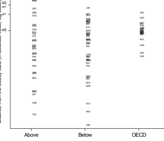
out that all OECD counties and 41 countries have the negative values and the remaining 32 countries have the positive values. We, therefore, divide the sample into three subsamples; ‘OECD’ (22 countries), ‘Below’ (41 countries), and ‘Above’ (32 countries). Figure 6 shows a plot of the distance from the steady state for all of the countries in the sample (Appendix 2 gives country
names, country codes and subsample groups).10
9We assume that g is 0.02 as MRW (1992). 10When the mean value of |ln (k(0)/y(0))
i− ln si+ ln(ni+ g + δ)| is calculated over the
We estimate equations (23) and (25) both with and without an intercept.
We assume that g is 0.02 and δ is 0.05.11 Table 1 reports the results of OLS
regressions with robust standard errors.
The results support the Solow model for the ‘OECD’ and ‘Above’ samples. All of the coefficient estimates in the ‘OECD’ and ‘Above’ samples have the
signs predicted by the model. Although ln(ni+ g + δ) does not enter
signifi-cantly in the regressions with an intercept, all of the coefficient estimates in the
regressions without an intercept are statistically significant.12 The restrictions
on the coefficients are not rejected in the ‘OECD’ and ‘Above’ samples. The
goodness of fit measures are high (e.g., the raw R2 for the restricted
regres-sion is 0.61 for the ‘OECD’ sample and 0.62 for the ‘Above’ sample).13 Most
important, in the regressions without an intercept, the implied α is 0.31 for the ‘OECD’ sample and 0.35 for the ‘Above’ sample. The data, thus, strongly
support the prediction that α is 1/3.14
Contrary to the ‘OECD’ and ‘Above’ samples, the data for the ‘Below’ sam-ple fail to support the model. The estimates for the coefficient on ln k/y(60) and all of the estimates for the coefficients in the restricted regressions are sta-tistically insignificant. The restrictions on the coefficients are rejected. The
goodness of fit measures are low (e.g., the raw R2 for the restricted regression
is 0.01). Most important, the implied α of 0.08 in the regression without an intercept is far below the prediction.
1960.
11We assume that δ is 0.05 as Barro and Sala-i-Martin (1992a, 1992b). They used the
value reported by Jorgenson and Yun (1986, 1990).
12If the intercept term is in fact absent as the specification suggests, the slope coefficients
may be estimated with far greater precision than with the intercept term left in. Table 1 shows that the intercept terms in the “OECD” and “Above” samples are insignificant not even at the 10 per cent significance level. Thus, one cannot reject the hypothesis that the true intercept is equal to zero, thereby justifying regression through the origin. In the case of the “Below” sample, the estimation shows that the intercept term is significant at the 1 per cent level. As it is discussed later, this can be additional evidence that the data for the “Below” sample does not support the Solow model.
13The values of raw R2 are calculated according to the definition: Raw R2
= 1 − (1 −Piei/PiYi), where e is the residual from the regression without an intercept and
Y is the dependent variable observed.
14One of the main reasons that MRW (1992) reject the strict Solow model is that the
estimated α for the Solow model without introducing human capital is much too high to be consistent with the conventional value of capital share.
Dependent Variable: (log difference GDP per working-age person 1960-85) - 0.5 Sample (obs): OECD(22) Above(32) Below(41) Regression with an intercept
constant 0.62 (1.33) −0.68 (3.57) 5.43∗∗∗ (2.05) ln(k/y 60) −0.61∗ (0.30) −0.45∗∗∗ (0.13) −0.25 (0.22) lns 1.20∗∗ (0.45) 0.57∗∗∗ (0.09) 0.65∗∗ (0.28) ln(n+g+δ) −0.64 (0.48) −0.86 (1.60) 1.78∗ (0.96) R2 0.48 0.54 0.40 Restricted regression: constant −0.13 (0.17) 0.02 (0.08) −0.07 (0.11) ln(k/y 60)-lns+ln(n+g+δ) −0.67∗ (0.35) −0.56∗∗∗ (0.07) −0.21 (0.27) R2 0.33 0.51 0.02
Test of restriction: p-value 0.10 0.54 0.00
Implied α 0.40 0.36 0.17
Regression without an intercept
ln(k/y 60) −0.60∗∗ (0.28) −0.45∗∗∗ (0.13) −0.19 (0.25) lns 1.14∗∗ (0.40) 0.57∗∗∗ (0.08) 0.66∗∗ (0.31) ln(n+g+δ) −0.85∗∗∗ (0.28) −0.56∗∗∗ (0.11) −0.58∗∗ (0.27) Raw R2 0.71 0.65 0.31 Restricted regression: ln(k/y 60)-lns+ln(n+g+δ) −0.44∗∗∗ (0.10) −0.54∗∗∗ (0.05) −0.09 (0.18) Raw R2 0.61 0.62 0.01
Test of restriction: p-value 0.10 0.51 0.01
Implied α 0.31 0.35 0.08
Notes: s=the average share of real investment in real GDP,k/y(60)=the capital-output in 1960,n=the average rate of growth of the working age population,g=0.02, and
δ=0.05. Robust standard errors are in parentheses. ∗ significant at 10% level,
∗∗significant at 5% level and ∗∗∗ significant at 1% level.
4
Empirical Test 2
4.1
The Specification
In this section, we perform another empirical test of the Solow model by es-timating the speed of convergence towards the steady state. We derive the empirical specifications below.
From equation (12), the convergence coefficient is given by:
β(t) = (1− α)(n + g + δ) µ y∗(t) y(t) ¶1−α α . (27)
Taking logs of equation (27) gives:
ln β(t) = ln(1− α) + ln(n + g + δ) − 1− α
α (ln y(t)− ln y
∗(t)) . (28)
From equation (22), we can obtain:
ln y∗(t) = ln y(0)− α 1− αln k(0) y(0)+ α 1− αln s− α 1− αln(n + g + δ) + g t. (29)
Substituting this expression into equation (28) and arranging it yield: ln µ y(t) y(0) ¶ i = α 1− αln(1− α) − α 1− αln βi(t) + git −1 α − αln µ k(0) y(0) ¶ i + α 1− αln si. (30)
The term, βi(t), in the equation (30) is not directly observable. Hence, we
estimate the generalized value of βi(t)across countries.
From equation (27), denoting (y∗(t)/y(t))
i as zi(t), we can rewrite βi(t)as: βi(t) = (1− α)(n + g + δ + eni+egi) (z(t) +zei(t))
1−α α ,
where n is the mean population growth rate,eni is the deviation from n, z(t) is
the mean of (y∗(t)/y(t))
i, and zei(t) is the deviation from z(t). We then define
the generalized value of βi(t) as below:
β(t) = (1− α)(n + g + δ)z(t)1−αα .
ln eβi(t) = ln βi(t)− ln β(t) = ln µ n + g + δ +eni+egi n + g + δ ¶ + 1− α α ln µ z(t) +zei(t) z(t) ¶ . (31)
A first order Taylor-Series expansion of ln((n + g + δ +eni +egi)/(n + g + δ))
around gi = g gives: ln µ n + g + δ +eni+egi n + g + δ ¶ ' ln µ n + g + δ +eni n + g + δ ¶ + egi n + g + δ +eni . (32)
Similarly, a first order Taylor-Series expansion of ln ((z(t) +zei(t))/z(t))around
zi(t) = z(t) gives: ln µ z(t) +zei(t) z(t) ¶ ' zez(t)i(t). (33)
By substituting equations (32) and (33) into equation (31), we can get:
ln βi(t) = ln β(t) + ln µ n + g + δ +eni n + g + δ ¶ + egi n + g + δ +eni +zei(t) z(t). Substituting this into equation (30) gives:
ln µ y(t) y(0) ¶ i − g t = 1 α − α ¡ ln(1− α) − ln β(t)¢− α 1− αln µ k(0) y(0) ¶ i + α 1− αln si− α 1− αln µ ni+ g + δ n + g + δ ¶ + εi, (34) where εi = µ t− α 1− α 1 ni+ g + δ ¶ egi− α 1− α e zi(t) z(t). (35)
The restricted version of equation(34) is given by:
ln µ y(t) y(0) ¶ i − g t = 1 α − α ¡ ln(1− α) − ln β(t)¢ − α 1− α µ ln µ k(0) y(0) ¶ i − ln si+ ln µ ni+ g + δ n + g + δ ¶¶ + εi. (36)
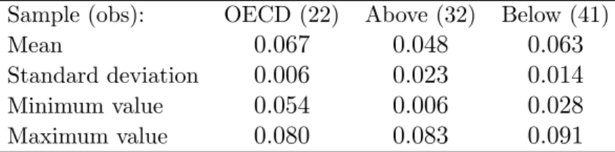
Sample (obs): OECD (22) Above (32) Below (41)
Mean 0.067 0.048 0.063
Standard deviation 0.006 0.023 0.014
Minimum value 0.054 0.006 0.028
Maximum value 0.080 0.083 0.091 Table 2: The calculated β values
Equations (34) and (36) are the regression specifications used in this
sec-tion. We treat εi as the error term and it is given by equation (35). As in
Section 3, we assume thategi is random and countries are close enough to their
steady states at year t so that most of the variation in zei(t) is due to demand
shocks.
The implication of equation (34) is similar to that of equation (23). It implies conditional convergence. By estimating equation (36) with OLS, we can get the estimate for α/(1 −α). This, in turn, gives the estimate for β(t) by
looking at the estimate for the constant term, (α/(1−α))¡ln(1− α) − ln β(t)¢.
As mentioned before, our main goal here is to check the validity of the Solow model by looking at the estimated value of α, which should be about 1/3.
4.2
Results
Before estimating equations (34) and (36), we provide a supplement for the regression tests. By substituting 0 for t in equation (28) and using equation (26), we can obtain: ln β(0)i = ln(1− α) − ln µ k(0) y(0) ¶ i + ln si. (37)
Assuming α = 1/3, we can calculate ln β for each country by using equation (37). We then calculate β(0) by simply taking the mean value across countries. Taking 1985 as the initial year, Table 2 gives the results.
Table 2 reports that the calculated β value in year 1985 is 0.067 for the ‘OECD’ sample, 0.048 for the ‘Above’ sample and 0.063 for the ‘Below’ sample. Thus, if the model describes the mechanism of economic growth well, the OLS regression estimates on equation (36) should be able to give the estimated β values that are close to the values of β reported in Table 2 and also give the estimated α values which are close to 1/3.
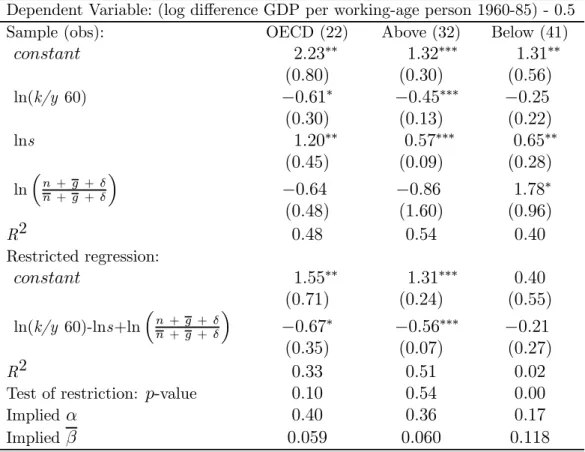
The regression results based on specifications (34) and (36) are given in Table 3. The results show that the data for the ‘OECD’ and ‘Above’ samples
Dependent Variable: (log difference GDP per working-age person 1960-85) - 0.5 Sample (obs): OECD (22) Above (32) Below (41)
constant 2.23∗∗ (0.80) 1.32∗∗∗ (0.30) 1.31∗∗ (0.56) ln(k/y 60) −0.61∗ (0.30) −0.45∗∗∗ (0.13) −0.25 (0.22) lns 1.20∗∗ (0.45) 0.57∗∗∗ (0.09) 0.65∗∗ (0.28) ln ³ n + g + δ n + g + δ ´ −0.64 (0.48) −0.86 (1.60) 1.78∗ (0.96) R2 0.48 0.54 0.40 Restricted regression: constant 1.55∗∗ (0.71) 1.31∗∗∗ (0.24) 0.40 (0.55) ln(k/y 60)-lns+ln ³ n + g + δ n + g + δ ´ −0.67∗ (0.35) −0.56∗∗∗ (0.07) −0.21 (0.27) R2 0.33 0.51 0.02
Test of restriction: p-value 0.10 0.54 0.00
Implied α 0.40 0.36 0.17
Implied β 0.059 0.060 0.118
See notes to Table 1. Data here are identical except fornwhich is the average ofnin each subsample.
Table 3: The test of the Solow model (Test 2)
seem to support the Solow model. All of the coefficient estimates for the two samples have the signs predicted by the model and most of them are
statistically significant.15 The restrictions on the coefficients are not rejected
in the ‘OECD’ and ‘Above’ samples, and the values of R2 are reasonably high.
Most important, the implied values of β for the ‘OECD’ and ‘Above’ samples are reasonably close to the values shown in Table 2 and the implied values of
α are very close to the conventional value of capital share.
In the case of the ‘Below’ sample, the results in Table 3, however, do
not support the model. The coefficient on ln ((ni+ g + δ)/(n + g + δ)) is of
the wrong sign and significant. The estimate for the coefficient on ln k/y(60)
15The robust standard errors of the coefficient on ln ((n
i+ g + δ)/(n + g + δ)) are large
in the ‘OECD’ and ‘Above’ samples. This could be because the constant term, (α/(1 − α))¡ln(1 − α) − ln β(t)¢, and ln ((ni+ g + δ)/(n + g + δ)) are both functions of n + g + δ.
in the unrestricted regression and all of the estimates for the coefficients in
the restricted regression are statistically insignificant. The R2 of 0.02 in the
restricted regression is poor and the restrictions are rejected. The implied β is far from the value shown in Table 2 and the implied α is about half the size of the conventional value of capital share.
5
Implication of the Obtained Results
The results from Sections 3 and 4 show that the Solow model explains the growth mechanism for the ‘OECD’ and ‘Above’ samples quite well but not for the ‘Below’ sample. In this section we examine the origins of these differences and provides a possible explanation.
The empirical tests conducted in the previous sections control for saving rates, population growth rates and initial levels of technology. The rates of technology growth are, however, left untouched and unobservable differences in technology growth rates are reflected in the error terms. Despite no con-ditioning on the rates of technology growth, convergence is observed in the ‘OECD’ and ‘Above’ samples but not in the ‘Below’ sample. If the Solow model describes the mechanism of economic growth correctly, the significant differences in convergence patterns across subsamples can be attributed to the fact that the growth rates of technology vary randomly in the ‘OECD’ and ‘Above’ samples but not in the ‘Below’ sample. The rates of technological progress may systematically differ across the ‘Below’ sample countries.
If technological progress is, as argued above, important for explaining the empirical results, we need to explain why the growth rates of technology sys-tematically vary only in the ‘Below’ sample. Many explanations are possible.
One of the most promising might be technology diffusion.16 In order to
incor-porate the idea of technology diffusion, we modify the assumptions about tech-nological progress. Firstly, we assume that there is one techtech-nologically leading country and the others are followers. As before technology is assumed not to be a worldwide good but rather a domestic good. However, this time, assume that technology diffusion from the leader benefits some countries. Some coun-tries can easily absorb cutting-edge technologies and make full use of them. Adoption of leading technologies can push the country’s technology level up over time. A larger gap in the initial technology level between the leader and the follower leads to a greater increase in the follower’s level of technology over time due to technology diffusion. This seems reasonable if we think about
im-16Barro and Sala-i-Martin (1997), for example, show the model in which technology
6 7 8 9 ln A (60) A bo v e Be low OECD
Figure 7: The distribution of A(0)
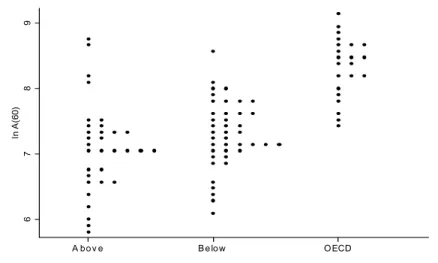
itation of technology. The rates of technology growth, thus, systematically differ across those countries who benefit from technology diffusion. On the other hands, if the follower initially has a similar level of technology as the leader, there is not much to be adopted or imitated by the follower. Thus, the rates of technology growth do not systematically differ across those countries who do not benefit much from technology diffusion. We also assume that it is hard for the follower to adopt or imitate the leading technologies if the follower does not have a baseline technology level since the follower would face a large adoption cost. Here, we interpret ‘technology’ in a broad sense. The initial level of technology A(0) reflects not just production technology but also in-stitutions, geographies, government policies and also possibly human capital. For example, a bad government policy set a barrier to technology adoption by increasing the amount of investment required for adopting leading technolo-gies. Thus, no or very little technology diffusion occurs in the countries with the very low levels of A(0). Parente and Prescott (1999) emphasize the role of barriers that limit firms’ incentives to adopt technology.
If the assumptions above are approximately correct, we should observe that the levels of A(0) of the ‘Below’ sample countries tend to be between those of the ‘OECD’ and ‘Above’ samples. Figure 7 shows the distributions of A in year 1960 for each sample group, where A(0) is calculated by using equation (21). It shows that the levels of ln A(0) of the ‘OECD’ sample countries are likely to be much higher than those of the other countries. It may thus be reasonable to say that many of the ‘OECD’ sample countries have the initial
levels of technology just below the leader’s ln A(0). As for other countries, it shows that the levels of ln A(0) of the ‘Above’ sample tend to be low and the levels of ln A(0) of the ‘Below’ sample tend to be between those of the other
two subsamples.17
Our regression results also indicate the possibility that the growth rates of technology are not random and are negatively correlated with initial levels of technology in the ‘Below’ sample due to technology diffusion. Compared with the implied values of α for the ‘OECD’ and ‘Above’ samples, the implied value of α for the ‘Below’ sample is far off below the conventional value of capital share. The low implied value of α for the ‘Below’ sample can be interpreted as
the bias introduced by the correlation between ln(k(0)/y(0))i− ln si+ ln(ni+
g + δ) and ²i in equation (25).18 Denoting −α/(1 − α), the coefficient on
ln(k(0)/y(0))i− ln si+ ln(ni+ g + δ) in equation (25), as x, the degree of the
bias is shown by:
E(x)b − x = Covhln³k(0)y(0)´ i− ln si+ ln(ni+ g + δ), ³ t− 1−αα (n 1 i+g+δ) ´ egi i V arhln³k(0)y(0)´ i− ln si+ ln(ni+ g + δ) i .
Assuming egi is not correlated with ln si and ln(ni+ g + δ),we can get:
E(x)b − x = E³ln³k(0)y(0)´ iegi ´ ³ t− 1−αα E³n 1 i+g+δ ´´ V arhln³k(0)y(0)´ i− ln si+ ln(ni+ g + δ) i.
Since t − (α/(1 − α))E(1/(ni+ g + δ)) is likely to be positive, the direction
of the bias in the estimate of x depends on the sign of E(ln(k(0)/y(0))iegi).19
If egi is positively correlated with ln(k(0)/y(0))i, we get an upward bias in
the estimate of x (i.e., a downward bias in the estimate of α). Since A(0)i
is negatively correlated with ln(k(0)/y(0))i, we get a downward bias in the
estimate of α if egi is negatively correlated with A(0)i.20 Hence, the very low
17The average level of technology in 1960 is higher in the ‘Below’ sample although the
average level of output per working age population in 1960 is higher in the ‘Above’ sample.
18For empirical test 2, the bias is introduced by the correlation between
(ln (k(0)/y(0))i− ln si+ ln((ni+ g + δ)/(n + g + δ)) and εi in equation (36). 19The maximum value of 1/(n
i+ g + δ) in our sample is 13.67 and the minimum value is
8.96. We use the 25 years sample period so that t is 25. Thus, assuming α = 1/3, the value of t − (α/(1 − α))/(ni+ g + δ) is in the range between 18.17 and 20.52 in our sample.
20Since k(0)/y(0) = (A(0)/y(0))−(1−α)/α and ∂(A(0)/y(0))/∂A(0) = α/y(0) > 0, A(0) i
estimate of α for the ‘Below’ sample may suggest the existence of a strong
negative relationship between A(0)i andegi in the ‘Below’ sample countries.21
6
Conclusion
This paper analyzes the Solow model both empirically and theoretically by taking a new approach which yields some important implications.
First, it shows the importance of a variation in the initial level of technology in the Solow model. The steady state level of income per capita and the (non-steady state) growth rate of income per capita are sensitive to the initial level of technology. It also shows the nature of convergence from above in a much clearer way than in previous work. Countries converging from above could have positive growth rates of capital per labor for a relatively long period before reaching their steady state paths.
We also construct a new method to test the Solow model by allowing for cross-country differences in initial levels and growth rates of technology. The results show that the Solow model can explain well growth mechanisms only for the ‘OECD’ and ‘Above’ samples. Conditional convergence due to diminishing returns to capital is observed in these two subsamples. The implied value of the speed of convergence is about 0.06 and it is much higher than the conventional estimated value of 0.02. To the contrary, the results show no evidence of conditional convergence in the ‘Below’ sample. It is argued that the significant differences in convergence patterns across subsamples come from the fact that technology diffusion has a large impact mainly on the ‘Below’ sample countries.
21We could also get the downward bias in the estimate of α if the countries are far from
their steady states at the end of the sample period. However, this is unlikely to be the reason why the implied value of α for the ‘Below’ sample is much lower than the implied values of α for the other two samples. When the value of |((1 − α)/α) ln(y∗(t)/y(t))i| with
egi = g is calculated for all of the countries in the sample by using equation (26), the mean
value in the ‘Below’ sample is lowest and the standard deviation in the ‘Below’ sample is lower than that in the ‘Above’ sample.
Appendix 1: The speed of convergence,
β
The coefficient of the speed of convergence is given by:β(t)' −d · X(t) d X(t) =− d ³d (ln k∗(t)−ln k(t)d t ´ d (ln k∗(t)− ln k(t). (A.1)
Using the facts:
ln y(t) = (1− α) ln A(t) + α ln k(t)
and
ln y∗(t) = (1− α) ln A(t) + α ln k∗(t),
the distance between ln k∗(t) and ln k(t) is given by:
ln k∗(t)− ln k(t) = 1
α (ln y
∗(t)− ln y(t)) . (A.2)
Substituting equation (A.2) into equation (A.1) yields: β(t)' −d ³d (ln y∗(t)−ln y(t))d t
´
/d (ln y∗(t)− ln y(t))
=−d ³g− y(t)y(t)· ´/d (lnyy(t)∗(t)) = d ³y(t)y(t)· ´/d (lnyy(t)∗(t)). (A.3)
Since y(t) = A(t)1−αk(t)α, the growth rate of output per labor is given by:
· y(t) y(t) = (1− α)g + α · k(t) k(t). (A.4)
By using the equation for the capital accumulation, the growth rate of capital per labor is given by:
· k(t)
k(t) = s A(t)
1−αk(t)α−1− (n + δ). (A.5)
Substituting equation (A.5) into equation (A.4) yields: · y(t) y(t) = (1− α)g + α ¡ s A(t)1−αk(t)α−1− (n + δ)¢. (A.6) Since s A(t)−αk(t)α
− (n + g + δ) k(t) A(t)−1 = 0 at the steady state,
k∗(t)α−1 = n + g + δ
s k(t) A(t)
Solving this equation for A(t) and substituting it into equation (A.6) yield: · y(t) y(t) = (1− α)g + α Ã (n + g + δ) µ k(t) k∗(t) ¶α−1 − (n + δ) ! . (A.7)
Rewriting equation (A.2) gives: k(t) k∗(t) = µ y(t) y∗(t) ¶1 α . Substituting this expression into equation (A.7) yields:
· y(t) y(t) = (1− α)g + α Ã (n + g + δ) µ y∗(t) y(t) ¶1−α α − (n + δ) ! . (A.8)
By substituting equation (A.8) into equation (A.3), the coefficient for the speed of convergence is thus given by:
β(t)' d d lny∗(t)y(t) µ (1− α)g + α µ (n + g + δ)³yy(t)∗(t)´ 1−α α − (n + δ) ¶¶ = yy(t)∗(t) µ 1−α α α(n + g + δ) ³ y∗(t) y(t) ´1−2α α ¶ = (1− α)(n + g + δ)³yy(t)∗(t) ´α−1 α .
Appendix 2: Subsample groups of countries
N a m e C o d e G ro u p N a m e C o d e G ro u p N a m e C o d e G ro u p
A n g o la A G O A b ove A lg e ria D Z A B e low P a ra g u ay P RY B e low
B a n g la d e s h B G D A b ove A rg e ntin a A R G B e low P e ru P E R B e low
B ra z il B R A A b ove B e n in B E N B e low P h ilip p in e P H L B e low C a m e ro o n C M R A b ove B o liv ia B O L B e low R w a n d a RWA B e low
C e ntr. A fric a n R . C A F A b ove B o tsw a n a B WA B e low S in g a p o re S G P B e low
C h a d T C D A b ove B u ru n d i B D I B e low S o m a lia S O M B e low C o lo m b ia C O L A b ove C h ile C H L B e low S y ria S Y R B e low
C o n g o C O G A b ove C o sta R ic a C R I B e low T h a ila n d T H A B e low
C y p ru s C Y P A b ove C o te d ’Ivo ire C IV B e low To g o T G O B e low E g y p t E G Y A b ove D o m in ic a n R . D O M B e low A u s tra lia A U S O E C D
G h a n a G H A A b ove E c u a d o r E C U B e low A u s tria A U T O E C D
K e nya K E N A b ove E l S a lva d o r S LV B e low B e lg iu m B E L O E C D L ib e ria L B R A b ove E th io p ia E T H B e low C a n a d a C A N O E C D
M a d a g a s c a r M D G A b ove G u a te m a la G T M B e low D e n m a rk D N K O E C D
M a u ritiu s M U S A b ove H a iti H T I B e low F in la n d F IN O E C D M o z a m b iq u e M O Z A b ove H o n d u ra s H N D B e low Fra n c e F R A O E C D
M ya n m a r B U R A b ove H o n g K o n g H K G B e low G e rm a ny G E R O E C D
N ic a ra g u a N IC A b ove In d ia ID N B e low G re e c e G R C O E C D P a k is ta n PA K A b ove Is ra e l IS R B e low Ire la n d IR L O E C D
P a p u a N e w G u in e a P N G A b ove J a m a ic a J A M B e low Ita ly ITA O E C D
S e n e g a l S E N A b ove J o rd a n J O R B e low J a p a n J P N O E C D S o u th A fric a Z A F A b ove K o re a K O R B e low N e th e rla n d s N L D O E C D
S ri L a n ka L K A A b ove M a law i M W I B e low N e w Z e a la n d N Z L O E C D
Ta n z a n ia T Z A A b ove M a lay s ia M Y S B e low N o rw ay N O R O E C D Trin id a d T T O A b ove M a li M L I B e low P o rtu g a l P RT O E C D
Tu n is ia T U N A b ove M a u rita n ia M RT B e low S p a in E S P O E C D
U g a n d a U G A A b ove M e x ic o M E X B e low S w e d e n S W E O E C D U ru g u ay U RY A b ove M o ro c c o M A R B e low S w itz e rla n d C H E O E C D
Ve n e z u e la V E N A b ove N e p a l N P L B e low Tu rke y T U R O E C D
Z a ire Z A R A b ove N ig e r N E R B e low U . K . G B R O E C D Z a m b ia Z M B A b ove N ig e ria N G A B e low U .S .A . U S A O E C D
References
Aghion, Philippe and Peter Howitt, “A Model of Growth through Creative Distruction,” Econometrica, March 1992, 60 (2), 323—351.
Barro, Robert J. and Jong-Wha Lee, “Sources of Economic Growth,” Carnegie Rochester Conference Series on Public Policy, June 1994, 40, 1—46.
and Xavier Sala-i-Martin, “Convergence across States and Regions,” Brookings Papers on Economic Activity, 1991, 1, 107—182.
and , “Convergence,” Journal of Political Economy, April 1992,
100 (2), 223—251.
and , “Regional Growth and Migration: A Japan-United States
Comparison,” Journal of the Japanese and International Economies, De-cember 1992, 6 (4), 312—346.
and , Economic Growth, New York: McGraw-Hill, 1995.
and , “Technological Diffusion, Convergence and Growth,” Journal
of Economic Growth, March 1997, 2 (1), 1—26.
Benhabib, Jess and Jordi Gali, “On Growth and Indeterminacy: Some Theory and Evidence,” Carnegie Rochester Conference Series on Public Policy, December 1995, 43, 163—211.
Bond, Stephen, Anke Hoeffler, and Jonathan Temple, “GMM Estimation of Empirical Growth Models,” 2001. Centre for Economic Policy Research Discussion Paper No.3048.
Caselli, Francesco, Gerardo Esquivel, and Fernando Lefort, “Reopening the Convergence Debate: A New Look at Cross-Country Growth Empirics,” Journal of Economic Growth, September 1996, 1 (3), 363—389.
Cho, Dongchul and Stephen Graham, “The Other Side of Conditional Con-vergence,” Economics Letters, February 1996, 50 (2), 285—290.
Durlauf, Steven N., “On Growth and Indeterminacy: Some Theory and Ev-idence - A Comment,” Carnegie Rochester Conference Series on Public Policy, December 1995, 43, 213—223.
, Paul A. Johnson, and Jonathan R. W. Temple, “Growth Econometrics,” 2004. Vassar College Department of Economics Working Paper Series No.61.
Grossman, Gene and Elhanan Helpman, Innovation and Growth in the Global Economy, Cambridge: MIT Press, 1991.
Hall, Robert E. and Charles I. Jones, “Why Do Some Countries Produce So Much More Output Per Worker Than Others?,” Quarterly Journal of Economics, February 1999, 114 (1), 83—116.
Islam, Nazrul, “Growth Empirics: A Panel Data Approach,” Quarterly Jour-nal of Economics, November 1995, 110 (4), 1127—1170.
, “What Have We Learnt from the Convergence Debate?,” Journal of Economic Survey, July 2003, 17 (3), 309—362.
Jorgenson, Dale W. and Kun-Yung Yun, “Tax Policy and Capital Allocation,” Scandinavian Journal of Economics, 1986, 88 (2), 355—377.
and , “Tax Reform and U.S. Economic Growth,” Jounal of Political
Economy, Part 2, October 1990, 98 (5), 151—193.
King, Robert G. and Ross Levine, “Capital Fundamentalism, Economic Devel-opment, and Economic Growth,” Carnegie Rochester Conference Series on Public Policy, June 1994, 40, 259—292.
Lee, Kevin, M. Hashem Pesaran, and Ron Smith, “Growth and Convergence in a Multi-Country Empirical Stochastic Solow Model,” Journal of Applied Econometrics, 1997, 12 (4), 357—392.
, , and , “Growth Empirics: A Panel Data Approach: A
Com-ment,” Quarterly Journal of Economics, February 1998, 113 (1), 319—323. Mankiw, Gregory N., David Romer, and David Weil, “A Contribution to the Empirics of Economic Growth,” Quarterly Journal of Economics, May 1992, 107 (2), 407—437.
Parente, Stephen L. and Edward C. Prescott, “Barriers to Technology Adop-tion and Development,” Journal of Political Economy, April 1994, 102 (2), 298—321.
Romer, Paul M., “Endogenous Technological Change,” Journal of Political Economy, Part 2, October 1990, 98 (5), 71—102.
, “The Origins of Endogenous Growth,” Journal of Economic Perspec-tives, Winter 1994, 8 (1), 3—22.
Solow, Robert M., “A Contribution to the Theory of Economic Growth,” Quarterly Journal of Economics, February 1956, 70 (1), 65—94.
Summers, Robert and Alan Heston, “The Penn World Table (Mark5): An Ex-panded Set of International Comparisons, 1950-1988,” Quarterly Journal of Economics, May 1991, 106 (2), 327—368.
Temple, Jonathan, “The New Growth Empirics,” Journal of Economic Lit-erature, March 1999, 37 (1), 112—156.
Wacziarg, Romain, “Review of Easterly’s The Elusive Quest for Growth,” Journal of Economic Literature, September 2002, 40 (3), 907—918.