The Effects of Corporate Finance on Firm
Risk-taking and Performance : Theory and
Evidence
journal or
publication title
Discussion paper series
number
45
page range
1-39
year
2009-05
DISCUSSION PAPER SERIES
Discussion paper No.45
The Effects of Corporate Finance on Firm
Risk-taking and Performance: Theory and Evidence
Toshihiro Okada Kwansei Gakuin University
Kohei Daido Kwansei Gakuin University
May 2009
SCHOOL OF ECONOMICS
KWANSEI GAKUIN UNIVERSITY
1-155 Uegahara Ichiban-cho Nishinomiya 662-8501, Japan
The Effects of Corporate Finance on Firm
Risk-taking and Performance: Theory and Evidence*
Toshihiro Okada
†Kwansei Gakuin University
Kohei Daido
‡Kwansei Gakuin University
Abstract
Some firms may exhibit better operating performance than others because they undertake riskier projects: risk-return tradeoff. We develop a model to examine the effects of financial contracts on a firm’s choice between safer (lower risk, lower return) and riskier (higher risk, higher return) projects. The model shows that, assuming a competitive capital market (i.e., financiers with no monopoly power), three types of financial contracts can each be an equilibrium contract, depending on conditions. We show that firms undertake “safer” projects when using rollover loans (i.e., short-term loans with a possible rollover option), while firms undertake “riskier” projects when using non-rollover loans (i.e., long-term loans) or new share issues. The model emphasizes the role of rollover loans (with passive monitoring) as a potential disciplinary device to suppress a firm’s risk-taking. The model gen-erates several predictions about the determinants of a firm’s risk-taking and its performance. One key prediction of the model is that (risk-neutral) firms with closer bank relationships are more likely to use rollover loans and undertake “safer” projects, even with a contestable capital market. We find novel empirical support for the model’s predictions.
JEL Classification: G32
Key Words: corporate finance, corporate governance, firm risk-taking, firm perfor-mance, loan rollover
†. [email protected] ‡. [email protected]
*We would like to especially thank Yoshiko Sato, whose help and advise have been invaluable to us. We would also like to thank Yuichi Abiko, Atsuo Fukuda, Ryoji Odoi, Hiroshi Osano, Ken Tabata, Yoshiro Tsutsui, Hirofumi Uchida, Kazuhiro Yamamoto, Noriyuki Yanagawa, and the seminar participants at Kobe University, Kwansei Gakuin Universitry, Osaka Prefecture University, and Osaka University for their useful comments and suggestions.
1
Introduction
To explain the operating performance of a firm, we usually consider its efficiency. A more efficient firm obtains more from a given amount of resources. Many studies have looked at firm performance through this lens. Researchers have considered various factors (e.g., inadequate production technologies, insufficient managerial efforts, perks, and under- and over-investment) to be a potential source of firm inefficiency and have investigated what mechanisms might help reduce these inefficiencies.1
Apart from efficiency, a firm’s risk-taking behavior can also be an important deter-minant of its operating performance.2 Some firms may exhibit better performance than
others simply because they undertake riskier business operations: risk-return tradeoff.3
In general, a firm has many different product lines and departments. A firm’s business operation can thus be viewed as a collection of many different individual activities with their own risk-return characteristics. Then, by applying the well-known theory of port-folio selection in finance, we can say that by diversification a firm faces a set of business operations on the efficient frontier–the frontier is, in the present context, the set of risk-return choices from the business operation opportunity set where for a given vari-ance (risk) no other business operation opportunity offers a higher expected return, and the frontier is monotonically increasing in the (variance, expected return) space. This means that a firm gets higher expected returns by choosing a riskier business operation. Conditions and events that change a firm’s risk-taking behavior can therefore alter its performance. In this paper, we focus on this risk-taking channel to study firm operating performance. In other words, we consider movement along the efficiency frontier rather than a shift in the frontier.4
Although various factors affect the risk-taking channel, corporate governance is prob-ably one of the most important. Suppose that a firm has two projects (two business operations): the "safe" project and the "risky" project. The safe project has the lower expected returns and the fewer risks, and the risky project has the higher expected re-turns and the more risks. If the firm’s financier prefers the safe project and the corporate 1See, for example, Jensen and Meckling (1976) on perks and over-investment, Myers (1977) on
under-investment, Myers and Majluf (1984) on under-under-investment, Jensen (1986) on free cash flows, Stultz (1990) on over- and under-investment, and Aghion and Bolton (1992) on perks.
2By "risk-taking", we mean the extent to which a firm is willing to engage in conduct with an
uncertain outcome for the firm.
3Gilley, Walters, and Olson (2002) investigate the influence of the risk-taking propensity of top
management teams on firm performance. They show that managerial risk-taking has a strong positive influence on firm performance. The recent study reported by John, Litov, and Yeung (2008) examines managerial incentives to take value-enhancing risks in relation to the investor protection environment. They find that better investor protection leads to higher firm risk-taking and, consequently, greater growth.
4Our paper differs from "under-investment" and "over-investment" stories, which focus on efficiency.
In addition, while the over-investment (asset substitution effects) story of Jensen and Meckling (1976) and the under-investment (debt overhang) story of Myers (1997) are about the agency cost of debt financing, we stress the benefit of debt financing to investors.
governance works well, the firm is disciplined to take the safe project even if it is risk neutral and thus prefers the risky project.
Considering the impact of corporate governance on the risk-taking channel, it is not hard to imagine that a financial contract plays a crucial role in determining a firm’s risk-taking behavior. A key aspect of corporate governance is how a firm’s financiers obtain a return on their investment. The first step to assure this return is to deliberately design a financial contract. A well-designed financial contract can establish effective corporate governance, and thus have an impact on a firm’s choice between safer (lower risk, lower return) and riskier (higher risk, higher return) business operations. This paper examines the effects of a financial contract on a firm’s risk-taking, which in turn affects its performance.
We develop a model to study the effects of a financial contract on a firm’s choice be-tween safer (lower variance, lower expected return) and riskier (higher variance, higher expected return) projects. The model assumes, for simplicity, that a risk-neutral firm has two projects: the "safe" project and the "risky" project, where the former has the lower expected return and the lower variance while the latter has the higher expected return and the higher variance. We consider a situation in which the firm requires financing from a risk-neutral competitive investor (competition exists between multiple principals: multiple bank investors and equity investors). In the model, (in which the firm’s action is unverifiable,) the firm prefers the risky project, but the bank investor wants the firm to choose the safe project; i.e., an agency problem exists between the firm and the bank investor (in contrast, no agency problem exist between the firm and the equity investor). The model shows that three types of (exclusive) financial contracts can each be an equilib-rium contract, depending on various conditions. The three contracts are: (i) a bank loan contract with an unconditional early loan demand option (i.e., an unconditional early liquidation option), (ii) a bank loan contract without the early demand option, and (iii) an equity contract. The second and third contracts are considered a long-term (normal) loan and a new share issue, respectively. The first contract is considered a short-term loan with a possible loan rollover. Rollover loans are commonly found in banking.
We argue that, while a firm undertakes a project with higher expected returns and more risks when choosing a normal (non-rollover) loan or a new share issue, it undertakes a project with lower expected returns and fewer risks when choosing a rollover loan. The loan contract with the early loan demand option (the early liquidation option) in the model preserves the most important feature of a rollover loan; i.e., a bank’s total control over continuation of the project implemented by the borrowing firm. In reality, a bank often refuses to roll-over maturing short-term loans.5 In the model, the early loan demand
option is not contingent on the firm’s action (playing it safe or risky) because the action 5The rollover condition is very often not written in a contract, but a bank and its borrower both
is unverifiable. The bank holding the contract can thus liquidate the project early at will. At first glance, it seems hard for the loan contract with the early demand option to be the equilibrium contract of the model because: (i) the agency problem exists between the firm and the bank investor (but not between the firm and the equity investor), (ii) the firm chooses any of the three competitive contracts, and (iii) the bank with the demandable loan contract can liquidate the project early at will. We will show, however, that under certain conditions the firm selects the early demandable loan contract in equilibrium.
There are three crucial and necessary reasons why, under certain conditions, the loan contract with the early demand (at will) option becomes an equilibrium contract and the risk-neutral firm chooses the "safe" project with this contract. The first reason is concerned with the credibility of the contract. The model shows that the loan contract with the early demand option (which is offered by a bank investor) can be credible to the firm in two ways. It can be credible in the sense that the firm knows that the bank investor will liquidate the project if the firm chooses the risky project. It can also be credible in the sense that the firm knows that the bank will not liquidate the project (i.e., the bank will let the business go) as long as the firm chooses the safe project. The first form of credibility works as a disciplinary device to constrain the firm’s risk-taking, and the latter form of credibility makes the contract acceptable to the firm even though it gives the bank total control over the firm’s operation. The second reason why the early demandable loan contract can be an equilibrium contract relates to the cost of liquidating firm assets. Firm assets include intangible assets like firm-specific knowledge and know-how, so that the firm assets become much less valuable if they are taken over by the bank investor (i.e., the debt holder) upon default due to project failure. In the model of our paper, this leads the bank to strongly prefer the "safe" project to the "risky" project. The bank may thus have an incentive to offer an interest rate low enough for the firm to choose the early demandable loan contract, knowing that with this interest rate the contract is credible in the ways described above. The third reason is concerned with the dilution of manager shareholdings. In the model, the manager of the firm owns part of the firm’s shares. The new share issue dilutes the manager’s shareholdings and thus may lead the manager to prefer the bank loan to the new share issue.
Close analysis of the model reveals the relationship between a firm’s risk-taking (and thus its performance) and three key variables of the model. The three variables are: the firm’s relationship with banks, the number of the firm’s outstanding shares and the firm’s scale of production. The model predicts that, holding all other factors fixed, the extent of a firm’s risk-taking, and thus its operating performance, is negatively related to the closeness of its relationship with banks and the scale of its production and positively related to the number of its outstanding shares.
One key prediction of the model is that (risk-neutral) firms with closer bank rela-tionships are more likely to use rollover loans and undertake "safer" business operations,
even with a contestable capital market. This prediction is partially attributed to het-erogeneous monitoring costs: in our model, bank investors having closer relationships with its client firms have informational advantages in passive monitoring (i.e., collect-ing information about firms) and the early liquidation by bank investors requires passive monitoring. If the prediction is correct, our model could explain an interesting fact about the distribution of firm ROA across countries. Kameda and Takagawa (2003) compare the distribution of ROA for Japanese firms with those observed for other countries, and find that the ROA distribution for Japanese firms has a much lower variance and mean than those observed for firms in other countries. This is consistent with the prediction that the closer relationship a firm has with banks, the safer and less profitable project the firm is likely to undertake. In fact, many Japanese firms are affiliated with a "main bank" and thus probably have a much closer relationship with banks than firms in other countries.
Using a panel of data obtained for Japanese firms, we find empirical support for the model’s predictions. Our empirical method has some new features. We show that al-though it is not possible to observe how much risk a firm has actually taken, a reasonable assumption about firm risk-taking and our newly proposed measure of performance un-certainty can together provide a reliable test of the model. We do not employ commonly used variables, such as the ex post variance of firm performance, in order to measure ex ante uncertainty of firm performance (i.e., ex ante risk). Using the ex post variance as a good proxy for ex ante uncertainty of firm performance requires a reasonable number of time-series observations of firm performance. This severely limits the number of usable observations for a regression, since usually only a short time-series of panel data on firm performance is available. The proposed method does not require many time-series obser-vations of firm performance to measure the uncertainty, so that the regressions can use a much lager number of time-series observations. In addition, we show that our method can provide a more accurate measure of the uncertainty. These features allow us to, in testing our model, reliably carry out a panel regression to control for a firm-specific effect, a time effect and a heterogeneous linear time trend (i.e., to control for unobserved firm efficiency), and thus mitigate the problem of omitted variable bias.
The most closely related work is a paper by Weinstein and Yafeh (1998). Using data on Japanese firms, they provide indirect evidence that banks exert pressure on their client firms and influence the firms to forgo high-risk, high-expected-return projects according to the bank’s preference.6 They argue that underdeveloped capital markets provide banks with monopoly power, and Japanese main banks have taken advantage of this situation and have suppressed a firm’s risk-taking behavior. Our study is complementary to their 6They find the lack of a significant advantage in growth rates for firms under main bank influence
and interpret this as evidence that main banks induce their client firms to take less risky projects which lead to lower growth rates.
work. The model of our paper shows that a bank may affect a client firm’s risk-taking be-havior even though a capital market is competitive, and the empirical test provides direct evidence of the effect of bank-firm relationships on firm risk-taking and performance.
Our study is related to the literature emphasizing the disciplinary role of debt in an incomplete contract setting. The literature includes Dewatripont and Tirole (1994), Berglof and von Thadden (1994), Zwiebel (1996), and Grinstein (2006), among many others.7 The paper differs from previous studies in a few important ways. First, our paper shows that the firm exhibits worse operating performance if it chooses a bank loan (debt) contract with disciplinary power over the firm. This result is different from that of other studies in which the debt contract disciplines the manager to work efficiently, and has a positive effect on firm performance. Second, the present paper differs in terms of allocation of control rights. In other studies, the debt holder is given control rights contingent on the verifiable outcome of default. In contrast, in our model the bank (the debt holder) can liquidate the project of its borrowing firm to demand an early loan payment at will. That is, the bank has non-contingent control rights.
The paper is also related to the work of Repullo and Suarez (1998) and Gordon and Kahn (2000). They also consider the disciplinary role of a loan contract with the option for a bank to liquidate its loan at will.8 Their treatment of the liquidation option differs
from ours. In Repullo and Suarez (1998), the option is exogenously included in a loan contract. In our paper, the option is endogenously included; i.e., the bank has a choice between including the option or not, and it decides by considering what other bank investors (and equity investors) would do. In Gordon and Kahn (2000), the liquidation is contingent on verifiable events. They assume that a bank loan contract includes a large number of covenants, such that a small change in the state of a borrowing firm will violate at least one covenant. This assumption makes it possible for a bank to execute its liquidation option at will at any time. In contrast, in our model, the execution of the option is not contingent on anything.
The outline of the paper is as follows: Section 2 presents a model of firm risk-taking and financial contracting, Section 3 discusses the empirical method and presents the results, and Section 4 concludes the paper.
7Earlier literature stressing the benefit of debt financing in mitigating an agency problem includes
Jensen and Meckling (1976) and Jensen (1986).
2
A Model of Firm Risk-taking and Financial
Con-tracting
2.1
Environment
Consider a firm run by a risk-neutral manager who owns a fraction of the firm’s shares (henceforth the "manager" and the "firm" are used interchangeably). Risk-neutral out-side investors own the remainder of the shares. The manager faces two projects, and both projects require the same set-up cost, I. For simplicity, we assume that the set-up cost is sunk. The two projects, project S and project R, are expected to be profitable and differ both in terms of riskiness and expected cash flow.
Project S and project R both generate three possible cash flow scenarios: 0 (fail), XL
(success) and XH (big success). We make the following assumption:
Assumption 1 XH > XL> I > 0.
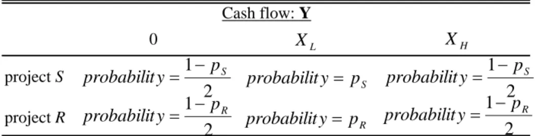
Table 1 shows the payoffs of the two projects. The manager is assumed to work efficiently, and the success probability pv in Table 1 is exogenously determined. According to Table
1, the expected cash flows from project S and that from project R are given by
E(Yv) = (1− pv) XH/2 + pv XL, v = S and R. (1)
The variances of the cash flows from the two projects are given by
var(Yv) = 1 4 £ (1− pv)((1 + pv)XH2 − 4pvXHXL+ 4pvXL2) ¤ , v = S and R. (2) We also make the following two assumptions
Assumption 2 pS > pR,
Assumption 3 XH− 2XL> 0.
Assumptions 2 and 3 give var(YR) > var(YS) and E(YR) > E(YS); i.e., project R is
riskier but generates a higher expected cash flow than project S.9 Projects R and S are considered to represent any pair of business operations on the efficiency frontier, which is the set of risk-return choices from the possible business operation opportunity set where, for a given variance (expected return), no other business operation opportunity offers a higher expected return (lower variance). The efficiency frontier is located in a different
9From (2) we can obtain var(Y
R) − var(YS) = 14(pS − pR)
h
(pS+pR)(XH-2XL)2+4(XH-XL)XL
i . Furthermore, from (1) we can obtain E(YR) − E(YS) = (pS− pR)(12XH− XL).
position if the exogenous variables take on different values. In other words, the firm’s efficiency level is exogenously given by I, pv, XL, and XH.
For convenience, we assume that the firm has no liabilities, has assets, A0, and requires
A0 to undertake its projects. The firm’s assets, A0, include intangible assets, factories,
machines, and land. To simplify the analysis, we disregard other kinds of assets such as cash on hand and marketable securities, so that the set-up cost, I, needs to be fully financed by outside investors. We also assume
Assumption 4 A0 < I and 1 < A0 ≤ A0
where A0 is the minimum amount of A0 for a firm to be in operation. Assumption 4
indicates that the investors face a risk of losing their investment.
The manager chooses either project S or project R. The manager either borrows from a single bank investor or issues shares to new outside investors in order to finance the project (i.e., the bank loan and equity contracts are exclusive). We assume that the investors are competitive.
2.2
Preliminary Model
We first present the preliminary model in which the loan contracts do not posses an early demandable loan option. Studying this simple model will facilitate a clearer understand-ing of the model later presented.
2.2.1 Model timing and contract types
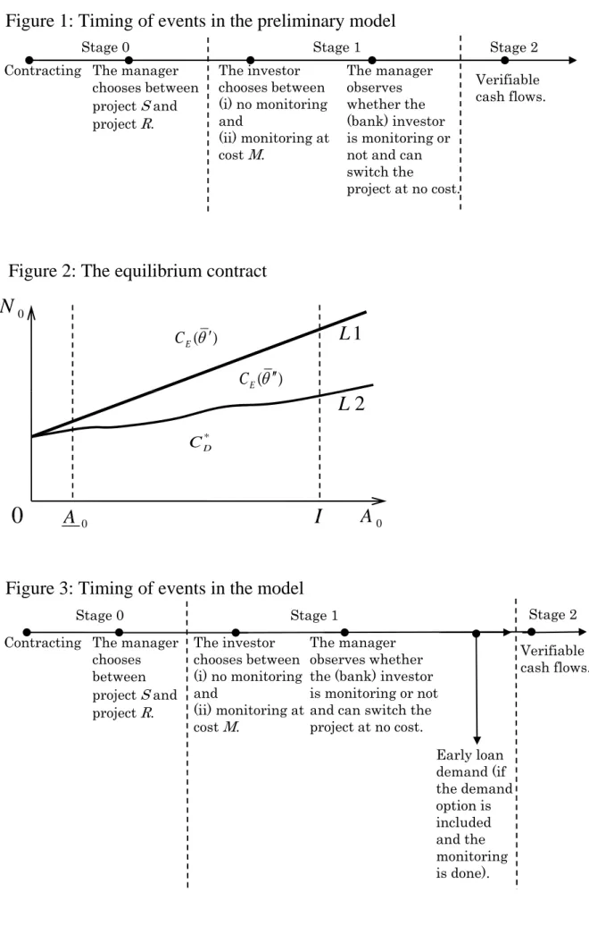
Figure 1 describes the timing of the preliminary model. The time line is divided into three stages: stage 0, stage 1 and stage 2.
(Stage 0) The contract is made and the firm receives funding.10 The manager then chooses between project S and project R. We assume that the manager’s project choice is unverifiable. Thus, a contract contingent on project choice (e.g., a contract that reads "if the firm does not undertake project S, the firm faces a large penalty") cannot be made.
(Stage 1) The investor chooses whether to monitor the firm at cost M (>0). The mon-itoring cost, M , differs among the investors. The manager can observe this monmon-itoring activity at no cost. The equity investor carries out active monitoring and the bank in-vestor performs passive monitoring. That is, the equity inin-vestor can directly interfere with the management of the firm and correct the course of action taken by the manager (if the investor owns a large proportion of the shares), while the bank investor can only 10Before this stage, the manager asks multiple banks for a loan and at the same time considers issuing
collect information about the firm’s activities (the information includes whether the firm is pursuing project S or project R). We assume that although the monitoring reveals the firm’s action (whether it is pursuing project S or project R) to the bank investor, the action is still unverifiable. This implies that the bank investor cannot write a contract contingent on the firm’s project choice. Therefore, the monitoring is useless to the bank investor in the present setting; i.e., the bank investor has no incentive to monitor the firm. However, a bank’s passive monitoring plays an important role in the model later presented: the model in which the loan contracts can posses an early demandable loan (at will) option. We also assume that in stage 1 the firm can change the project at no cost after observing whether the bank investor has chosen to monitor or not.
(Stage 2) The verifiable cash flows are realized. Since the cash flows are verifiable, to place the manager in an optimal incentive scheme, the bank investors can, in principle, write a contract contingent on the project cash flows. We assume, however, that the bank investors do not want to write the contingent contract because writing such a contract is too costly. That is, the cost associated with verifying the firm’s outcome (realized cash flow in the model) at the end of the period is assumed to be much higher than the cost of writing a simple loan contract without costly verification. The bank loan contracts hereafter do not require any verification of the firm’s outcome. Note also that verifiability of cash flow is necessary because an equity contract is included in the model. Equity contracting is not possible without verifiability of cash flow.
The equity contract, CE, and the loan contract, CD, are defined as
CE = CE(θ), CD = CD(r),
where θ is the manager’s shareholding ratio after new shares of the firm are issued and r is the interest rate. The bank investor with CD has the right to seize the firm’s assets
upon default of the firm. The equity investor, on the other hand, does not have this right. We first consider equity contracting. We assume that there are a number of homoge-nous equity investors, and that the investor cannot finance the project alone. If the manager decides to issue new shares (i.e., the manager decides to obtain funds from the equity investors), he has the following expected net return by undertaking project v
πM(θ:v) = θ[pv (A0+ XL) +1−p2v(A0+ XH) +1−p2vA0] − θ0A0
= θ(A0+ E(Yv))− θ0A0, v = S and R,
(3) where θ0 is an initial shareholding ratio of the manager (the manager’s shareholding ratio
before new shares of the firm are issued). The term in [ ] shows the expected value of the firm. The term θ0A0 represents the value that the manager obtains if project v is not
undertaken; i.e., θ0A0 is the manager’s reservation level of utility.
obtains the following expected return (if he does not monitor the firm, i.e., if he does not pay M ) πEI(θ:v) = 1q[pv (1− (θ + eθ))(A0+ XL) +1−pv 2 (1− (θ + eθ))(A0+ XH) + 1−pv 2 (1− (θ + eθ))(A0)] −I q, v = S and R, (4)
where q is the number of homogeneous equity investors, and eθ is a shareholding ratio for the initially existing equity investors after new shares of the firm are issued. The term eθ can thus be written as a function of θ and θ0, i.e., eθ = eθ(θ, θ0). The term in [ ] represents
the expected value of the firm if project v is undertaken, and Iq represents the amount of investment made by the investor. Notice here that how many shares of the firm the representative equity investor offers to purchase by paying Iq is the same thing as CE(θ)
being offered to the manager by the homogeneous equity investors as a whole. Equations (3) and (4) give
πM(θ:R) − πM(θ:S) = (pS− pR) θ 2 (XH− 2XL), (5) πEI(θ:R) − πEI(θ:S) = (pS− pR)(1− θ) 2 (XH− 2XL). (6)
From Assumptions 2 and 3, πM(θ:R) − πM(θ:S) > 0 and πEI(θ:R) − πEI(θ:S) > 0; i.e.,
the equity investor and the manager both prefer project R to project S. Thus, an agency problem does not arise in this case and the equity investor has no incentive to monitor the firm.
Next, consider bank loan contracting. If the bank investor makes a loan to the firm, the bank has the following expected return11
πBI(r:v) = pv rI + 1− pv 2 rI + 1− pv 2 (A0− I − A w 0 ), v = S and R, (7) where 0 < w < 1, (8) rI ≤ XL− I. (9)
The term (A0− I − A0w)in (7) shows what the investor obtains if the project fails (i.e.,
if the project cash flow is zero). The term A w
0 represents the cost of liquidating firm
assets. Since assets A0 include intangible assets like firm-specific knowledge and
know-how, the assets becomes much less valuable if they are taken over by the bank investor upon default due to failure of the project. The term A w
0 captures this wedge between the
bank investor and the manager in the valuation of A0 . It can also include the transaction 11Note also that if rI > X
L− I, then, πBI is, in some cases, not defined by (7). However, we can
cost of liquidating A0, e.g., the cost of selling assets to third parties. This type of cost
can also be quite large.12
If the firm borrows from the bank investor, the manager has the following expected net return by undertaking project v
πM(r:v) = θ0[pv(A0+ XL− (1 + r)I) + 1−p2v(A0+ XH− (1 + r)I)]
− θ0A0, v = S and R.
(10) As in the case of equity contracting, the term in [ ] and θ0A0 show the expected value of
the firm and the manager’s reservation level of utility, respectively. Equations (7) and (10) give
πM(r:R) − πM(r:S) = pS− pR 2 θ0 [XH− 2XL+ (1 + r)I− A0] , πBI(r:R) − πBI(r:S) = − pS− pR 2 [(1 + r)I− A0+ A w 0 ] .
From Assumptions 2, 3, and 4, πM(r:R) − πM(r:S) > 0 and πBI(r:R) − πBI(r:S) < 0.
This means that, although the bank investor wants the manager to choose project S, the manager has an incentive to choose project R. An agency problem thus arises in the case of bank loan contracting. The important point here is the role of A w
0 . Although
the existence of the agency problem does not hinge on the wedge A w
0 (i.e., the agency
problem arises even if A0w = 0), the bank’s preference for project S over project R is
stronger with A0w. This point will be very important when we later analyze the model
with the early loan demand option. 2.2.2 Equilibrium contracts
We now analyze the preliminary model and demonstrate the equilibrium contracts. First, we consider the loan contract, CD. Since the manager has an incentive to choose project
Rin the loan contract and the bank investor figures this out, the bank investor knows that πBI (r:R) is the only possible return. Thus, for the bank investor to have an incentive to
offer the loan contract, the following constraint must hold
πBI(r:R) ≥ a, (11)
where a is the net return on investing I on risk-free assets and E(Yv)− I > a.13 From
(7) and (11), we obtain r≥ 1 1 + pR [2a I + (1− pR)− 1− pR I (A0− A w 0 )] . (12)
12See Tirole (2006, pp. 164-171) for more concrete arguement of this kind of costs. 13Since a is the net return on risk-free assets, it is natural to assume E(Y
Under investor competition, the bank investor needs to offer the CD which maximizes
the manager’s expected profits, in order for the contract to be accepted. Thus, we can obtain the following lemma
Lemma 1 The contract which the bank investor offers is given by
C∗D= CD(r), (13) where r = 1 1 + pR [2a I + (1− pR)− 1− pR I (A0− A w 0 )], (14) πBI(r:R) = a, (15) πM(r:R) = θ0[E(YR)− 1− pR 2 A w 0 − I − a]. (16)
Proof. Proof in the text. C∗
D is a feasible contract, assuming that πM(r:R) ≥ 0 holds. The term "feasible
contract" means that by signing such a contract, the manager and investor both obtain the expected profits which are greater than or equal to their reservation levels. The contract is not feasible if either the manager or the investor gets (knows that he gets) less than the reservation level by signing it. The interest rate r is greater than zero based on Assumption 4.
Next, consider the equity contract CE. For the equity investor to have an incentive
to invest I
q, the following constraint must hold
πEI(θ:R) ≥
a
q. (17)
From (4) and (17), we can then get I + a
A0 + E(YR) ≤ 1 − [θ + eθ(θ, θ
0)]. (18)
The term 1 − [θ + eθ(θ, θ0)]shows a shareholding ratio for the new equity investors. Since
the firm must issue at least one share to each of the homogeneous equity investors, the following inequality must also hold
q
N0+ q ≤ 1 − [θ + eθ(θ, θ
0)], (19)
where N0 is the number of shares initially issued (the number of shares outstanding before
Under investor competition, θ must take the highest possible value. Using (18) and (19), the contract which the equity investor offers is thus given by
C∗E = CE(θ), where 1− [θ + eθ(θ, θ0)] = I + a A0+ E(YR) if q N0+ q < I + a A0+ E(YR) , (20) 1− [θ + eθ(θ, θ0)] = q N0+ q if q N0+ q > I + a A0+ E(YR) . (21)
Now denote θ0 as the θ in (20). Using (3), we can then obtain πM(θ
0
:R) = (A0+ E(YR)) θ 0
− θ0A0. (22)
Appendix A shows that θ0 is given by θ0 = θ0
A0+ E(YR)− (I + a)
A0+ E(YR)
. (23)
Substituting (23) into (22) for θ0 yields πM(θ
0
:R) = θ0[E(YR)− (I + a)].
This result is as expected since the new equity investor receives just the reservation level. Consequently, we can establish that
Lemma 2 If Nq
0+q <
I+a
A0+E(YR), the contract which the equity investor offers is given by
C∗E = CE(θ 0 ), where θ0 = θ0 A0+ E(YR)− (I + a) A0+ E(YR) , πM(θ0:R) = θ0[E(YR)− (I + a)], πEI(θ 0 :R) = a q. Proof. Proof in the text.
The contract CE(θ0) in Lemma 2 is a feasible contract since π M,EI(θ 0 :R) > 0 and πEI(θ 0 :R) = aq.
Similar to the analysis above, we denote θ00 as the θ in (21). We then can obtain the following lemma.
Lemma 3 If Nq
0+q >
I+a
A0+E(YR), the contract which the equity investor offers is given by
C∗E = CE(θ 00 ), where θ00 = F0 N0 + q , πM(θ 00 :R) = θ0 1 N0+ q [N0E(YR)− qA0] , πEI(θ 00 :R) = 1 q ∙ q N0+ q (A0+ E(YR))− I ¸ . Here, F0 is the number of the shares which the manager owns.
Proof. Proof in Appendix B. In Lemma 3, πEI(θ 00 :R) > a q, since q N0+q > I+a
A0+E(YR). That is, the equity investor
obtains more than the reservation level even under competition. Assuming that q is not large (i.e., q < N0E(YAR)
0 , where E(YR) A0 > 1), πM(θ 00 :R) > 0.14 Thus, CE(θ 00 ) is a feasible contract.
We are now in a position to examine the equilibrium contracts of the model. Proposition 1 (i) If Nq
0+q <
I+a
A0+E(YR), CE(θ
0
) is the equilibrium contract. (ii) If Nq
0+q > I+a A0+E(YR) and 1−pR 2 A w 0 + (a + I)− q N0+q(A0 + E(YR)) > 0, CE(θ 00 ) is the equilibrium contract. (iii) If Nq 0+q > I+a A0+E(YR) and 1−pR 2 A w 0 + (a + I)− q N0+q(A0+ E(YR)) < 0, CD(r)
is the equilibrium contract. Proof. (i) From Lemma 2, ifNq
0+q <
I+a
A0+E(YR), CE(θ
0
)is the contract offered by the equity investor. As already shown, CD(r) and CE(θ
0
) are feasible contracts. From Lemmas 1 and 2, we can obtain
πM(θ 0 :R) − πM(r:R) = θ0 1− pR 2 A w 0 .
This is greater than 0. Thus, the manager prefers CE(θ 0
) to CD(r).
(ii) and (iii) From Lemma 3, if Nq
0+q >
I+a
A0+E(YR), CE(θ
00
) is the contract offered by the equity investor. As already shown, CD(r) and CE(θ
00
) are feasible contracts. From Lemmas 1 and 3, we can obtain
πM(θ 00 :R) − πM(r:R) = θ0 ∙ 1− pR 2 A w 0 + (a + I)− q N0+ q (A0+ E(YR)) ¸ .
This can be negative or positive. Since θ0 > 0, πM(θ 00 :R) − πM(r:R) > 0 (< 0) if 1−pR 2 A w 0 + (a + I)− q
N0+q(A0+ E(YR)) > 0 (< 0). Thus, the manager prefers CE(θ
00
)to 14Together with q
N0+q >
I+a
A0+E(YR), we thus assume
N0 E(YR)
A0 > q >
N0 (I+a)
A0+E(YR)−I−a, where
E(YR)
A0 >
I+a
CD(r) if 1−p2RA0w+ (a + I)− q
N0+q(A0+ E(YR)) > 0, and the manager prefers CD(r) to
CE(θ 00 )if 1−pR 2 A w 0 + (a + I)− q N0+q(A0+ E(YR)) < 0.
Proposition 1 is visualized as in Figure 2. In the figure, the straight line (L1) at the top is given by N0 = q a + I(A0 + E(YR))− q, µ ⇔ N q 0+ q = I + a A0+ E(YR) ¶ . (24)
Another line (L2) is given by N0 = q 1−PR 2 A w 0 + a + I (A0+ E(YR))− q, (25) µ ⇔ 1− pR 2 A w 0 + (a + I)− q N0+ q (A0 + E(YR)) = 0 ¶ .
L1 and L2 never cross, and L2 is below L1 for A0 ≤ A0 < I.15 Figure 2 shows that
CD(r) is the equilibrium contract when N0 is small, such that N0q+q > A0+E(YI+a
R) and 1−pR 2 A w 0 + (a + I)− q
N0+q(A0 + E(YR)) < 0. This is because dilution of the manager’s
shareholdings by issuing new shares is large if N0 is low (i.e., θ0 − θ is large if N0 is
low), so that the manager prefers CD(r) to CE. However, when the manager realizes
the dilution is large, such that πM(θ 00
:R) − πM(r:R) < 0, he can, in principle, split the
shares first and then issue new shares. This procedure can provide the manager with πM(θ
0
:R) because splitting the shares allows manager to drive down πEI(θ:R) to the
equity investor’s reservation level a
q without affecting the manager’s shareholding ratio.
This ends up being the case of Nq
0+q <
I+a
A0+E(YR), because splitting the existing shares
before issuing the new shares implies an increase in N0: the equilibrium contract will
then be CE(θ 0
). We assume that there is a cost to share-splits, and this hinders the manager from splitting the shares. Appendix C shows the effect of the costs in detail. It shows that if the costs are higher than θ0((1− pR)/2)Iw, the manager does not consider
splitting the shares.16
15At A
0 = 0, the two lines intersects with each other.
h ∂³q¡1−PR 2 A w 0 + a + I ¢−1 (A0+ E(YR)) − q ´ /∂A0 i ³ q a+I ´−1 −1 = © -Aw
0 (1 − pR)£2aA0 + A01+w(1 − pR) + 2A0I + 2awA0 + 2wA0I + 2awE(YR) + 2wE(YR)I¤ª /
[2(a + I) + Aw
0 (1 − pR)]2. The right hand side of this equation is less than
zero. Thus,h∂³q¡1−PR 2 A w 0 + a + I ¢−1 (A0+ E(YR)) - q ´ / ∂A0 i
< a+Iq . Note here that h ∂³q¡1−PR 2 A0w+ a + I ¢−1 (A0+ E(YR)) - q ´ / ∂A0 i
can be negative or positive. Line L2 in Figure 2 represents the case ofh∂³q¡1−PR
2 A w 0 + a + I ¢−1 (A0 + E(YR)) - q ´ / ∂A0 i > 0.
16McGough (1993) and Angel (1997) argue that the costs of splitting shares (e.g., administrative
costs, transfer tax, and printing costs) can be substantial. Bebartzi, Michaely, and Weld (2007) report that firms almost never split their shares in Japan.
2.3
The Model
We have shown that the loan contract and the equity contract can each be an equilibrium contract, but that the contract type does not matter in the manager’s project choice. The manager always plays it risky (chooses project R). In this subsection, we show that the manager, in some cases, plays it safe (chooses project S) by selecting the loan contract.
Remember that the bank investor faces an agency problem. To overcome the problem, he devises a way to discipline (threaten) the manager. Otherwise, the manager will never play it safe (i.e., never choose project S). To discipline the manager, the bank investor must provide a credible threat to the manager by including some sort of option in the loan contract.
Since the firm’s action–to make "safe" or "risky" choices–is not verifiable, and the bank never wants to write a contract contingent on the project outcome (because it is too costly), the option must be a non-contingent one. Although the option could take any form, it is reasonable to suppose that the bank investor thinks of including a non-contingent early loan demand option in the contract; i.e., an option for the investor to liquidate the project early at will. This loan contract can be interpreted as a short-term loan with a possible rollover, which is common in banking. Most commercial bank loans are, in fact, of the short-term type, and banks often refuse to roll over maturing short-term loans. The contract with the early loan demand option preserves the most important feature of a rollover loan; i.e., a bank’s total control over continuation of the project implemented by its borrowing firm.
At first glance, it seems hard for the loan contract with the early demand option to be an equilibrium contract because: (i) the agency problem exists between the firm and the bank investor (but not between the firm and the equity investor), (ii) the firm chooses any of the three competitive contracts, and (iii) the bank with the demandable loan contract can liquidate the project early at will. We will show, however, that under certain conditions, the firm selects the loan contract with the early demand option and plays it safe in equilibrium.
2.3.1 Model timing and contract types
Model timing is slightly changed from the preliminary model, as shown in Figure 3. In contrast to the preliminary model, early loan demand is now possible during stage 1 if the option is written in the contract and passive monitoring is implemented. If the project is liquidated in stage 1, the firm receives no cash flow. Here we assume that the liquidation requires monitoring because the bank investor must know about the firm (e.g., it must know where the assets are placed) in order to intervene and seize the assets. In other words, passive monitoring makes it possible for the bank investor to liquidate the project
early.17
The equity contract is the same as the one shown in the preliminary model. The loan contract is now defined by
CD= CD(r, L, Z) ,
where L denotes the early liquidation option (L = 1 if the option is included and L = 0 otherwise), and Z is the payment received by the bank from the firm in liquidation of the project. Z may include collateral. If L = 0, Z = 0, and Z > 0 if L = 1. Note here that the firm never wants its project to be liquidated because, if the project is liquidated early, it receives no cash flow and must pay Z > 0. For analytical convenience, we divide CD
into two types: a type A loan contract and a type B loan contract. The type A contract, CDA, has L = 0, and the type B contract, CDB, has L = 1. Thus, they can be written as
CDA = CDA(r) and CDB = CDB(r, Z).
CDA is identical to the loan contact studied in the preliminary model. Thus, an
immediate corollary arises from Lemma 1:
Corollary 1 If the bank investor does not include the early loan demand option, the contract which the bank investor offers is given by
CD∗A = CDA(r), where r= 1 1 + pR [2a I + (1− pR)− 1− pR I (A0− A w 0 )], πBI(r:R) = a, πM(r:R) = θ0[E(YR)− 1− pR 2 A w 0 − I − a], and C∗ DA is a feasible contract.
Consider next CDB. The bank investor with CDB has three possible returns: πBI(r:R),
πBI(r:R) − M, and πBI(r:S) − M. Return πBI(r:S) is not possible because: (i) the
man-ager knows that the bank needs to monitor the firm in order to liquidate the project early, (ii) the manager can switch the project after observing whether the bank is monitoring or not, and (iii) the manager, with a given interest rate, prefers project R to project S.18 With a given interest rate, π
BI(r:R), πBI(r:R) − M, and πBI(r:S) − M are ordered
17As we will show later, this gives the bank investor an incentive to monitor the firm. In contrast, in
the preliminary model, the bank does not have an incentive to monitor and thus no monitoring occurs.
18In fact, (ii) with (i) is the same as assuming that the bank can (contractually) commit to monitor
the firm because the contractual commitment also makes it impossible for the bank to obtain πBI(r:S).
according to either ⎧ ⎪ ⎪ ⎪ ⎨ ⎪ ⎪ ⎪ ⎩ πBI(r:R) − M < πBI(r:R) < πBI(r:S) − M or πBI(r:R) − M < πBI(r:S) − M < πBI(r:R). (26)
In the following, we examine the feasibility of CDB, using (26) in relation to the bank
investor’s reservation level of utility, a.
Before examining the feasibility of CDB, we rule out the cases which clearly lead to
non-equilibrium CDB, in order to simplify our analysis of the model. With πBI(r:R) ≥ a,
Corollary 1 gives
πM(r:S) < πM(r:R) ≤ πM(r:R) . (27)
Expression (27) tells that the manager prefers C∗
DA to CDB(r, Z)with {(r, Z) | πBI(r:R) ≥
a}.19 Thus, under investor competition where any bank can offer C∗DA, CDB(r, Z) with
{(r, Z) | πBI(r:R) ≥ a} cannot be the equilibrium contract of the model, even if it
is a feasible contract. In the following analysis, we can thus safely ignore the case of πBI(r:R) ≥ a.
To analyze the feasibility of CDB, we first consider CDB(r, Z) with {(r,Z) | πBI(r:R)
< a and πBI(r:S) - M <a}. With this contract, (26) can be rewritten as
⎧ ⎪ ⎪ ⎪ ⎨ ⎪ ⎪ ⎪ ⎩ πBI(r:R) < πBI(r:S) − M < a. or πBI(r:S) − M < πBI(r:R) < a. (28)
Expression (28) indicates that the bank has no incentive to offer CDB(r, Z) with {(r,Z)
| πBI(r:R) <a and πBI(r:S) - M <a} unless a ≤ Z − M. From (28), the CDB(r, Z)
with a ≤ Z − M implies that the investor liquidates the project regardless of whether the manager plays it safe or risky. Therefore, since the liquidation provides the manager with return less than his reservation level, then CDB with {(r,Z) | πBI(r:R) < a and πBI(r:S)
- M < a} cannot be a feasible contract.
Next, consider CDB(r, Z) with {(r,Z) | πBI(r:R) < a and πBI(r:S) - M ≥ a}. For
bank cannot be credible under any circumstances because, from an ex post perspective, the bank investor has no incentive to monitor the firm. This leads to the result that CDBcannot be the equilibrium contract
of the model. Khalil (1997) and Khalil and Parigi (1998) study this kind of commitment problem and analyze a mixed-strategy equilibrium. In order to keep the model simple, we have decided not to follow this approach. Many studies, e.g., Diamond (1991), Rajan (1992) and Repullo and Suarez (1998), make the assumption that the bank can commit to monitor.
19To be precise, this arguement is not exactly correct. C∗
DAand the CDB which gives the manager the
same level of return as C∗
DAare indifferent for the manager in terms of his expected monetary return. We
this contract, (26) can be rewritten as
πBI(r:R) − M < πBI(r:R) < a ≤ πBI(r:S) − M . (29)
Considering (29), we can establish the following lemma
Lemma 4 CDB(r, Z) (excluding CDB(r, Z) with {(r, Z) | πBI(r:R) ≥ a}) is a feasible
contract only if it is with
{(r, Z) | πBI(r:R) < a ≤ πBI(r:S)− M, πBI(r:R) < Z < πBI(r:S)} , (30)
and, if the manager ever accepts feasible CDB(r, Z), he or she undertakes project S.
Proof. To examine the feasibility of CDB(r, Z) with {(r, Z) | πBI(r:R) < a ≤ πBI(r:S)
-M }, we consider (i) Z ≤ πBI(r:R), (ii) Z ≥ πBI(r:S) and (iii) πBI(r:R) < Z < πBI(r:S)
in turn (note that these three cases cover every possibility, since πBI(r:R) < πBI(r:S)).
First, consider the case of Z ≤ πBI(r:R). If Z ≤ πBI(r:R), Z − M ≤ πBI(r:R) − M.
From (29), we then obtain
Z − M ≤ πBI(r:R) − M < πBI(r:R) < a ≤ πBI(r:S) − M .
This expression indicates that the bank investor has no incentive to liquidate the project because doing so results in the lowest return (Z −M). With this knowledge, the manager plays it risky if he accepts the contract. The investor thus gets πBI(r:R) − M < a.
Therefore, the CDB with Z ≤ πBI(r:R) is not a feasible contract (knowing that he
receives πBI(r:R) − M < a, the bank investor never offers this contract).
Second, consider the case of Z ≥ πBI(r:S). If Z ≥ πBI(r:S), Z − M ≥ πBI(r:S) −
M. From (29), we then obtain
πBI(r:R) − M < πBI(r:R) < a ≤ πBI(r:S) − M ≤ Z − M .
This expression implies that the bank investor liquidates the project regardless of what the manager does. Since the liquidation of the project gives the manager a return less than his reservation level, then the CDB(r, Z)with Z ≥ πBI(r:S) is not a feasible contract.
Finally, consider the case of πBI(r:R) < Z < πBI(r:S). If πBI(r:R) < Z < πBI(r:S),
πBI(r:R) − M < Z − M < πBI(r:S) − M . (31)
With this contract, the bank investor’s best choice of action is to monitor the firm, and the liquidation threat becomes credible. The reasoning is as follows. If the bank does not monitor, it gets a return less than the reservation level (πBI(r:R) < a from expression
manager plays it risky, according to (31): πBI(r:R) − M < Z − M. Since the manager
never wants to be liquidated, observing that the bank is monitoring and thus knowing that the bank is ready to liquidate the project, he does not play it risky.20 According to (31),
the bank then gets πBI(r:S) − M ≥ a, which is the highest possible return in this case.
This leads the bank and the manager to believe that the bank’s best choice of action is to monitor the firm, and thus the threat of liquidation becomes credible.21 As a result, the manager plays it safe, and the bank obtains πBI(r:S) − M ≥ a if the contract is signed.
This contract also provides another form of credibility. According to (31): Z − M < πBI(r:S) − M, the bank has no incentive to liquidate as long as the manager plays it safe
(bank monitoring reveals whether the manager is playing it safe or risky). In other words, the level of Z given by (30) makes the manager believe that the bank will not execute the liquidation option if the manager plays it safe. This makes the contract acceptable to the manager. CDB with (30) is thus a feasible contract (a ≤ πBI(r:S) − M in (30)
holds if M is not too large).
According to the previous analyses, CDB(r, Z)with {(r,Z) | πBI(r:R) < a and πBI(r:S)
- M < a} is not a feasible contract. CDB(r, Z)(excluding CDB(r, Z)with {(r,Z) | πBI(r:R)
≥ a}) is thus a feasible contract only if it is with {(r,Z) | πBI(r:R) < a ≤ πBI(r:S) - M ,
πBI(r:R) < Z < πBI(r:S)}, and the manager plays it safe if he accepts feasible CDB.
The important point in Lemma 4 and its proof is that a feasible type B loan contract is "credible" to the manager in two ways. First, it is credible in the sense that the manager knows that the bank investor will liquidate the project if the manager plays it risky. Second, the contract is credible in the sense that the manager knows that the bank investor will not liquidate the project (i.e., the bank will let the business go) as long as the manager plays it safe. The first form of credibility works as a disciplinary device for the manager, and the second form of credibility makes the contract acceptable to the manager, even though the contract gives the bank total control over the firm’s operation. By setting r and Z given by Lemma 4, CDB(r, Z) gains these two forms of
credibility at once. For example, with a given Z, CDB(r, Z) having a value of r that is
too high or too low neither disciplines the manager nor represents a feasible contract. Interestingly, with a given r, Z works as not only as a threatening device, but also as a relieving device for the manager by making the manager believe that the bank will not execute the liquidation option as long as he plays it safe.
Other important points are that, as mentioned in the proof of Lemma 4, a ≤ πBI(r:S) − M in (30) cannot hold if M is too large, and that the bank (weakly) prefers
feasible CDB(r, Z) to CDA(r) (see Corollary 1 and Lemma 4).
20Note that the manager’s observation of bank monitoring is important. The manager observes bank
monitoring, and this makes the manager believe that the bank is ready to liquidate the project if the manager does not behave himself (remember that monitoring is required for liquidation).
21This is not possible without the assumption that the manager can switch the project after observing
2.3.2 Different M
We have not yet considered bank competition in offering CDB(r, Z), although monitoring
cost M is assumed to differ among the investors. Consider the effects of such competition in the following.
There are many possible candidates that cause M to vary across banks. The most important factor is probably the bank’s relationship with the firm. We assume that the bank more closely tied to the firm has a lower level of M because the closer relationship leads to an informational advantage. For example, in Japan, it is common for banks to temporarily (typically for several years) transfer their executives to client firms as senior executives (sometimes even as board members), and also for client firms to hire the retired executives of their banks. Banks that send their executives to client firms are likely to pay lower monitoring costs than banks with no close connection with their client firms.
We define bank 1 as the bank with the closest relationship to the firm and bank 2 as the second closest one. We denote η as closeness, where a bank with a lower level of η is more closely tied to the firm. We then have
0 < η1 < η2 , (32)
where the subscript indicates bank 1 or bank 2. To simplify the analysis, we also assume
M = η . (33)
By defining rB as the interest rate that satisfies πBI(rB:S) − M = a and using (7) and
(33), we can obtain rB(η) =
1 (1 + pS)I
[(1− pS)(I − A0+ A0w) + 2(a + η)] . (34)
Since feasible CDB requires πBI(r:S) − M ≥ a according to Lemma 4, rB shows the lower
bound on r of feasible CDB for a given Z: as already shown by using (28), with r <rB
the bank liquidates the project early regardless of what the manager does. Equations (32) and (34) then provide the following inequality
rB(η1) < rB(η2) . (35) Now suppose bank 2 offers feasible CDB(r2, Z2), where r2 = rB(η2), that is, in offering
the contract, bank 2 sets the interest rate at the lowest possible level. By accepting this contract, the firm gets πM(r2:S) (remember from Lemma 4 that the manager chooses
the manager. For example, bank 1 can offer feasible CDB(r1, Z1), such that:
rB(η1)≤ r1 < r2 = rB(η2) and Z1 = Z2 .
The manager prefers the CDB(r1, Z1) to the CDB(r2, Z2), since πM(r2:S) < πM(r1:S).
22
Note here that the levels of Z1 and Z2 are irrelevant to the firm’s return as long as Z1 and
Z2 satisfy πBI(r:R) < Z < πBI(r:S) in (30) of Lemma 4 (i.e., as long as the contracts
are feasible). This is because if the manager accepts feasible CDB, he undertakes project
S and knows that the bank will not liquidate the project as long as he behaves himself (so that Z is not in his return function). We can thus establish that
Lemma 5 Bank 1 can offer feasible CDB which dominates any feasible CDB of bank 2.
Proof. Proof in the text.
An immediate corollary from Lemmas 4 and 5 is
Corollary 2 If CDB is ever signed, the contract is always the one offered by bank 1.
Bank 1 can offer feasible CDB(r1, Z1) if its monitoring cost (M1 = η1) is not large.
Bank 1 can obtain more than its reservation level if its feasible CDB is accepted by the
manager. In addition, bank 1 prefers feasible CDB(r1, Z1)to CD∗A because C
∗
DA gives bank
1 just the reservation level. 2.3.3 Equilibrium contracts
We can now examine the model’s equilibrium contracts. Since we are interested in know-ing under what circumstances the manager undertakes project S, we focus on findknow-ing the conditions for which feasible CDB(r1, Z1)becomes the equilibrium contract of the model.
To find the equilibrium conditions, we start by comparing feasible CDB(r1, Z1) with
the feasible CDA, C∗DA = CDA(r). Let us first define rB, such that
πM(r:R) = πM(rB:S).
As Corollary 1 shows, r is the interest rate of C∗
DA. Solving the equation for rB yields
rB =
1 (1 + pS)I
[(1− pR)A0w+ (1− pS)(I − A0) + 2a + (pS− pR)(2XL− XH)] . (36)
Only if feasible CDB(r1, Z1) has an interest rate less than rB, the manager prefers it to
CDA(r). Remember that rB(η1) is the lower bound on r1 of feasible CDB(r1, Z1). Thus,
22Although not directly comparable, this result and the implication of (35) seem to be consistent with
the findings of Petersen and Rajan (1994) and Berger and Udell (1995). They find that firms with closer bank relations are charged a lower interest rate.
for feasible CDB(r1, Z1) to be an equilibrium contract, it must have r1, such that
rB(η1) < r1 < rB . (37)
Bank 1 sets r1in the range given by (37). The level of r1selected from this range depends
on η2 and the upper bound on r1 of feasible CDB(r1, Z1).
23
Considering (37) and using (34) and (36), we can get the following necessary condition for equilibrium CDB(r1, Z1).
rB− rB(η1) =
1 (1 + pS)I
[(pS− pR)(A0w− (XH− 2XL)− 2η1] > 0. (38)
The term rB − rB(η1) cannot be positive without the wedge A0w. In other words, the
equilibrium condition cannot be met without A w
0 . This is because the bank’s preference
for project S over project R cannot be strong enough without A w
0 , and thus bank 1 has
no incentive to offer a type B contract with an r1 low enough to attract the manager.
To obtain the equilibrium conditions, we also need to compare feasible CDB(r1, Z1)
with feasible CE. Let us define r0E and r00E, such that
πM(θ 0 :R) = πM(rE0 :S), (39) πM(θ 00 :R) = πM(rE00:S) (40)
where θ0 and θ00 are given by Lemma 1 and Lemma 2, respectively. Solving equations (39) and (40) gives rE0 = 1 (1 + pS)I " 2(pS− pR)XL− (pS− pR)XH +(1− pS)(I − A0) + 2a # , (41) rE00 = 1 (1 + pS)I " E(YS)− NN0+q0 E(YR) + ³ 1+pS 2 − N0 N0+q ´ A0 −¡1+pS 2 ¢ I # . (42)
Remember from the analysis of the preliminary model that: (i) if Nq
0+q <
I+a A0+E(YR),
the equity investor offers CE (θ 0
), and (ii) if Nq
0+q >
I+a
A0+E(YR), the equity investor offers
CE(θ 00 ). (CE(θ 0 ) and CE(θ 00
) are feasible contracts.) Thus, since rB(η1) is the lower
bound on r1 of feasible CDB(r1, Z1), in order for feasible CDB(r1, Z1)to be an equilibrium
contract, it must have r1, such that
rB(η1) < r1 < rE0 if q N0+q < I+a A0+E(YR), rB(η1) < r1 < rE00 if q N0+q > I+a A0+E(YR). (43) 23We can derive the upper bound on r
From (34), (41) and (42), we can obtain r0E − rB(η1) = 1 (1 + pS)I " (pS− pR)(2XL− XH) −(1 − pS)A0w− 2η1 # , (44) r00E − rB(η1) = 1 (1 + pS)I " 2³E(YS)−NN0+q0 E(YR) ´ + N2q 0+qA0 −(1 − pS)A0w− 2(I + a + η1) # . (45)
The values for rE0 −rB(η1)in (44) cannot be positive, since pS−pR> 0from Assumption 2,
2XL− XH < 0 from Assumption 3 and η1 > 0. Therefore, according to (43), CDB(r1, Z1)
cannot be an equilibrium contract if Nq
0+q <
I+a
A0+E(YR). Thus, the following necessary
conditions for equilibrium CDB(r1, Z1) are obtained
rE00 − rB(η1) = 1 (1 + pS)I ⎡ ⎢ ⎢ ⎣ 2³E(YS)− NN0 0+qE(YR) ´ +N2q 0+qA0− (1 − pS)A w 0 −2(I + a + η1) ⎤ ⎥ ⎥ ⎦ > 0, (46) q N0+ q > I + a A0+ E(YR) . (47)
In sum, we can establish that
Proposition 2 The conditions for equilibrium CDB(r1, Z1) are (all of the following
in-equalities must be met)
[(pS− pR)(A0w − (XH− 2XL)− 2η1] > 0, (48) " 2³E(YS)− NN0+q0 E(YR) ´ + N2q 0+qA0 −(1 − pS)A0w − 2(I + a + η1) # > 0, (49) q N0+ q − I + a A0+ E(YR) > 0. (50)
If CDB(r1, Z1) is the equilibrium contract, the manager undertakes project S.
Proof. Proof in the text.
The left hand sides of (48), (49) and (50) can be positive or negative. From the condition in Proposition 2, we can obtain the following set of equations.
∂CD0 ∂η1 = ∂CD00 ∂η1 =−2 (< 0), ∂CD00 ∂N0 =− q (N0+q)2 [A0+ E(YR)] (< 0), ∂CD000 ∂N0 =− q (N0+q)2 (< 0), ∂CD0 ∂A0 = wA w−1 0 (> 0), ∂CD00 ∂A0 = 2q N0+q − w(1 − pS)A w−1 0 , ∂CD000 ∂A0 = a+I (A0+E(YR))2 (> 0), (51)
where CD0, CD00 and CD000 are the left hand sides of (48), (49), and (50), respectively.
The signs of the values in (51) are shown in parentheses. Apart from ∂CD∂A00
0 , all of the
signs are singly determined, as shown in (51). 2.3.4 From the model to the empirical test
To test the model empirically, we make the following assumptions.
Assumption 5 For any given η1, A0, and N0, the probability that firm i has CD0 > 0,
CD00 > 0, and CD000 > 0 at time t is nonzero.
Assumption 6 η1, A0, and N0 are not correlated with the other variables.
Assumption 6 implies that η1, A0, and N0 are not correlated with the productivity
(efficiency) of the firm because pv, XL, XH, and I together reflect the productivity. Since
this may not be true in reality, using a panel of data for Japanese firms, our empirical tests attempt to control for differences in firm productivity by including a firm-specific effect, a time effect and a heterogeneous linear time trend.
Since (51) shows that ∂CD∂η 0
1 , ∂CD00 ∂η1 , ∂CD00 ∂N0 , and ∂CD000
∂N0 are all negative, assumptions 5
and 6 lead to the following corollary
Corollary 3 (i) Holding N0 and A0 fixed, the lower the level of η1, the more likely firm
i is to undertake project S at time t, and (ii) holding η1 and A0 fixed, the lower the level
of N0, the more likely firm i is to undertake project S at time t.
Although (51) shows ∂CD∂A 0
0 > 0 and
∂CD000
∂A0 > 0, the effect of A0 on the firm’s project
choice is not clear: ∂CD∂A00
0 can be negative or positive. We assume that
∂CD00
∂A0 > 0 holds
because our empirical test employs the data for firms with relatively large A0
N0 (relatively
high share prices) and, if A0
N0 is large,
∂CD00
∂A0 is positive according to (51). The model then
implies that holding N0 and η1 fixed, the higher the level of A0, the more likely firm i
is to undertake project S at time t. We would like to empirically test this together with Corollary 3.
Above all, we make the following testable hypotheses for the model:
Hypothesis 1 Holding all other factors constant, the closer relationship firm i has with banks, the safer but less profitable project firm i undertakes at time t,
Hypothesis 2 Holding all other factors constant, the lower the number of firm i’s out-standing shares, the safer but less profitable project firm i undertakes at time t,
Hypothesis 3 Holding all other factors constant, the lager the scale of firm i’s produc-tion, the safer but less profitable project firm i undertakes at time t.
When making these hypotheses, we interpret η1 as a firm’s relationship with its banks in general rather than with a single bank (we will show how this is measured later). This is because: (i) although in the model η1 is the firm’s relationship with bank 1 (the most
closely related bank), in reality it is often difficult to correctly identify which bank has the closest tie with the firm, and (ii) more importantly, firms, generally, borrow from several banks. Concerning N0 and A0, N0 is simply the number of outstanding shares of
a firm, and A0 represents the scale of a firm’s production since A0 is the assets required
to undertake the project (including both tangible and intangible assets).
3
Empirical Testing of the Model
In this section, we empirically test Hypotheses 1, 2, and 3. The testing consists of two parts. The first regression test considers firm i’s risk taking behavior (henceforth F RTi). The hypotheses suggest that F RTi is influenced by firm i’s relationship with its
banks, the number of firm i’s outstanding shares, and the scale of its production. The second regression test considers firm i’s operating profitability (ROAi: return on assets).
The hypotheses suggest that the three variables (firm i’s relationship with banks, the number of firm i’s outstanding shares, and the scale of its production) influence ROAi
through their effect on F RTi. As we will later show, the testing is an interactive two-step
procedure in which the first and second regression tests complement each other.
3.1
Specification of FRT regressions
We will now derive the regression specification for the first test. According to the hy-potheses, F RTi at time t can be given by
F RTi,t = cF RT + ζF RTi + λ F RT
t + α1 BRi,t+ α2 N Si,t+ α3 SCi,t, (52)
where cF RT is a constant effect across time and firms, ζF RT
i is a firm-specific effect, λ F RT t
is a time effect, BRi,t is firm i’s relationship with its banks at time t, N Si,t is the number
of outstanding shares of firm i at time t, and SCi,t is the scale of production for firm i at
time t. An increase in F RTi,t means that firm i takes more risks. An increase in BRi,t
indicates that firm i has a closer relationship with its banks (measured by a decrease in η1,i in the model). The hypotheses tell that α1 < 0, α2 > 0, and α3 < 0. We want to
estimate α1, α2, and α3, but F RTi,t is unobservable (we cannot observe how much risk
a firm has actually taken). We demonstrate a strategy to overcome this problem. Assume that the following relationship exists
Ei,t
£
where Ei,t is an expectation operator, φi,t+1 is the uncertainty of firm i’s profitability
at time t + 1 (i.e., the degree of deviation of ROAi,t+1 from Ei,t[ROAi,t+1]), cEF is a
constant effect across time and firms, ζEFi is a firm-specific effect, and λEFt+1 is a time effect. Ei,t
£ φi,t+1
¤
is the value of φi,t+1 that firm i expects at time t and Ei,t[λEFt+1] is
the value of λEFt+1 expected at time t. We believe that the assumed relationship of (53)
is reasonable. With α4 > 0, (53) shows that Ei,t
£ φi,t+1
¤
is positively related to F RTi,t:
taking more risks at time t, firm i expects that the uncertainty of its profitability will increase at time t + 1.
Next, by substituting (52) into (53) for F RTi,t, we obtain
φi,t+1= cF + ζFi + λFt + α4α1 BRi,t + α4α2 N Si,t+ α4α3 SCi,t+ εFi,t+1, (54)
where cF = α4cF RT + cEF, ζFi = α4ζF RTi + ζ EF i , λFt = α4λF RTt + λ EF t+1,
εFi,t+1= (φi,t+1− Ei,t
£
φi,t+1¤) + (λEFt+1− Ei,t[λEFt+1]). (55)
Equation (54) is our basic regression specification to test the hypotheses (we will later show how to measure φi,t+1).24 As (55) shows, the term εF
i,t+1 in (54) is the sum of firm
i’s expectation error for φi,t+1 and that for λEFt+1. Thus, treating εF
i,t+1 as an error term,
we can obtain unbiased coefficient estimates from the regression.
Estimating the coefficients of (54), we can test the relationship shown in (52). To test whether α1 < 0, α2 > 0, and α3 < 0 hold, we need only to check the estimates of α4α1,
α4α2, and α4α3 since we know α4 > 0. If the estimates for α4α1 and α4α3 are negative
and significant, and the estimate for α4α2 is positive and significant, partial evidence for
the model’ validity is obtained.
3.2
Specification of the firm profitability regressions
We next show the regression specification for the second test. In the first regression test, we examine whether BRi,t, N Si,t, and SCi,t have an effect on F RTi,t, as the model
predicts. However, this is not enough to prove the validity of the model. The model shows that BRi, N Si, and SCi influence ROAi through their effect on F RTi, i.e., through the
risk-taking channel.
24Some of the coefficients in (54) vary across firms and time because the values in (51) are not constant,
except ∂CD∂η 0
1 and
∂CD00
∂η1 . Since it is a formidable task to allow the coefficients to differ as shown by (51),
According to the hypotheses, we can obtain the following expression
Ei,t[ROAi,t+1] = cROAE+ ζROAEi + Ei,t[λROAEt+1 ] + β1 F RTi,t, (56)
where ROAi,t+1is firm i’s return on assets at time t + 1, cROAE is a constant effect across
time and firms, ζROAEi is a firm-specific effect, and λROAEt+1 is a time effect.25 E
i,t[ROAi,t+1]
is the value of ROAi,t+1that firm i expects at time t, and Ei,t[λROAEt+1 ]is the value of λ ROAE t+1
expected at time t.
Using (52) and (56), we can get
ROAi,t+1= cROA+ ζROAi + λ ROA
t+1 + β1 F RT[i,t+ εROAi,t+1, (57)
where
[
F RTi,t = [α4α1 BRi,t + [α4α2 N Si,t+ [α4α3 SCi,t
cROA = cROAE+ δcRT A, ζROAi = ζROAEi + δζRT Ai , λROAt = λROAEt+1 + δλRT At ,
εROAi,t+1 = (ROAi,t+1− Ei,t[ROAi,t+1]) + (λROAEt+1 − Ei,t[λROAEt+1 ]). (58)
Equation (57) is our basic regression specification. The values of [α4α1, [α4α2, and [α4α3
are the coefficient estimates from the first regression, and thus [F RTi,t reflects the part
of F RTi,t explained (predicted) by BRi,t, N Si,t, and SCi,t.26 If the hypotheses are valid,
we should find that β1 > 0. The term εROAi,t+1 in (57) is the sum of the two expectation
errors, as shown by (58). As before, treating εROA
i,t+1 as an error term, we can thus obtain
unbiased coefficient estimates.
The test is thus an interactive two-step procedure. First, we do the F RT regression and estimates the coefficients. Then, using the predicted value [F RT, we estimate β1.27
We need support from both tests in order to verify the validity of the model. 25As shown in the data appendix, ROA
t+1 is measured by (operating profits at t + 1)/(total assets
at time t).
26Although [F RT
i,t is α4 times the part of F RT predicted by the three variables, it does not matter
for the test of β1 in terms of sign and significance. This is because α4 only scales up the predicted part
of F RT .
27We could also directly include BR, N S and SC in the second regression test. However, this approach
would not correctly identify the effect of F RT on ROA, since these variables might influence ROA in other ways; e.g., SC might affect ROA through an economy of scale (the efficiency channel) rather than the risk-taking channel.