PDF file

Local Bernstein-Sato ideals:

An algorithm and examples

Rouchdi Bahloul

Universit´e de Lyon, Univ. Lyon 1, Institut Camille Jordan, CNRS UMR 5208, 43 Bd du 11 novembre 1918, F-69622 Villeurbanne, France

Toshinori Oaku

Department of Mathematics, Tokyo Woman’s Christian University, Suginami-ku, Tokyo 167-8585, Japan

Abstract

Let k be a field of characteristic 0. For a polynomial mapping f = (f1, . . . , fp) of kn to kp,

the local Bernstein-Sato ideal of f at a point a ∈ kn _{is defined as an ideal of the ring of}

polynomials in s = (s1, . . . , sp). We propose an algorithm for computing local Bernstein-Sato

ideals combining Gr¨obner bases in rings of differential operators and primary decomposition in a polynomial ring. It also enables us to compute a constructible stratification of kn such that the local Bernstein-Sato ideal is constant along each stratum. We also present examples, some of which have non-principal Bernstein-Sato ideals, computed with our algorithm by using a computer algebra system Risa/Asir.

Key words: Bernstein-Sato ideal, D-module, Gr¨obner base, primary decomposition

Introduction

Let n be a positive integer, k a field of characteristic zero, and a = (a1, . . . , an) a fixed point in kn. Let x = (x1, . . . , xn) be a set of indeterminates. In this introduction,

A shall be one of the following rings: the polynomial ring k[x]; the localization k[x]a of

k[x] at a; the formal power series ring ˆOkn_,a= k[[x− a]] = k[[x₁− a₁, . . . , xn− an]]; and

when k =C, the ring O_Cn_,a of germs of complex analytic functions at a. Denote by ∂_xi

Email addresses: [email protected] (Rouchdi Bahloul), [email protected] (Toshinori

Oaku).

URLs: http://math.univ-lyon1.fr/∼bahloul/ (Rouchdi Bahloul), http://lab.twcu.ac.jp/oaku/

the partial differential operator _∂x∂

i and by DA= A⟨∂x1, . . . , ∂xn⟩ the ring of differential

operators with coefficients in A.

Let p≥ 1 be an integer and let us consider f = (f1, . . . , fp)∈ Ap. Denote by F the product f1· · · fp and let us introduce a set of indeterminates s = (s1, . . . , sp) and the

A[1/F, s]-free module

LA= A[1/F, s]· fs with fs = fs1

1 · · · f

sp

p . The set LA is naturally endowed with a DA[s]-module structure. Indeed, given g∈ A[1/F, s], we have

∂x_i· gfs= (_∂g ∂xi + g p ∑ j=1 sj∂fj ∂xi f_j−1 ) fs.

The moduleLA is an interesting and important object not only in D-module theory but also in, e.g., algebraic geometry, the theory of prehomogeneous vector spaces, and the theory of hypergeometric functions in several variables. For example, Oaku and Takayama (1999) proposed an algorithm for computing the twisted de Rham cohomology groups of the complement of the affine hypersurface F = 0 inCnby using the D-module structure ofLA.

The Bernstein-Sato ideal of f (with respect to A) is defined to be the ideal BA(f ) ={b(s) ∈ k[s] | b(s)fs∈ DA[s]· F fs}

of k[s] and plays an essential role in studying the D-module structure ofLA. If p = 1, the monic generator ofBA(f ) is called the Bernstein-Sato polynomial of f (with respect to A) (see (Bernstein, 1972)). When f ∈ k[x]p,Bk[x](f ) is called the global Bernstein-Sato

ideal and Bk[x]a(f ) is called the local Bernstein-Sato ideal at a∈ k

n_{. It is easy to see} thatBk[x]a(f ) is equal toBOˆkn ,a(f ) and thatBC[x]a(f ) is equal toBOCn,a(f ) if f ∈ C[x]

p_. When f∈ O_Cn_,a,B_O

Cn,a(f ) is called the analytic Bernstein-Sato ideal of f , and it is equal toB_Oˆ

Cn,a(f ). Finally, when f ∈ ˆOkn,a, we callBOˆkn ,a(f ) the formal Bernstein-Sato ideal

of f (at a).

It was proved by Sabbah (1987) that analytic Bernstein-Sato ideals are not zero. See also (Bahloul, 2005a) for a constructive proof. Theoretical studies of Bernstein-Sato ideals can also be found in, e.g., (Maynadier, 1997), (Brian¸con and Maynadier, 1999), (Brian¸con and Maisonobe, 2002), (Bahloul, 2005b).

For a polynomial mapping, a general algorithm for the global Bernstein-Sato ideal was first proposed by Oaku and Takayama (1999); its modifications have been given by Bahloul (2001), Brian¸con and Maisonobe (2002), Levandovskyy and Morales (2008). On the other hand, for p = 1, Oaku (1997a) gave an algorithm for the local Bernstein-Sato polynomial at a given point (see also the recent work by Nakayama (2009)).

The first goal of the present paper is to present an algorithm for computingBk[x]a(f )

for a given f ∈ k[x]p_{with p≥ 1 and a ∈ k}n_{. For this purpose, we combine the algorithm} of Oaku and Takayama (1999) for the global Bernstein-Sato ideal, which is based on Gr¨obner base computations in rings of differential operators, with primary decomposition in a polynomial ring, in the same way as was proposed by Oaku (1997b) in the case p = 1. This algorithm also provides us with a constructible stratification of kn such that for a running over a given stratum the local Bernstein-Sato ideal at a is constant. The existence of such a stratification was proved theoretically by Brian¸con and Maisonobe (2002).

We have implemented our algorithm in a computer algebra system Risa/Asir (Noro el al.). Experimentation suggests that, at least in ‘simple’ cases, global and local Bernstein-Sato ideals are mostly principal, i.e., generated by a single element. In fact, Maynadier (1997) proved that the local Bernstein-Sato ideal is principal if n = p = 2 and f = (f1, f2) defines a quasi-homogeneous complete intersection with an isolated singularity. On the other hand, Brian¸con and Maynadier (1999) showed that the local Bernstein-Sato ideal of f = (z, x4_{+ y}4_{+ 2zx}2_y2_{) in three variables (x, y, z) at the origin is not principal} without giving its explicit generators. We can compute the two generators of it using our algorithm (see Example 3). Rather surprisingly, the global Bernstein-Sato ideal of the same f is principal. This exemplifies the importance of computing the local Bernstein-Sato ideal. We also present some variants of this example.

In Section 1, we describe fundamental properties and the algorithm. For the sake of clarity, all the proofs are postponed to Section 2. In Section 3, we give some examples computed with our algorithm (over the rationals) together with a validity proof of the results over the complex numbers. Finally in Section 4, we give some remarks on our implementation in Risa/Asir.

1. An algorithm for local Bernstein-Sato ideals

Let us fix a polynomial mapping f = (f1, . . . , fp) ∈ k[x]p. We are interested in

Bk[x]a(f ). As we recalled, the formal, analytic (if k =C), and local Bernstein-Sato ideals

of f at a are the same. So we shall use the notationBloc,a(f ) =Bk[x]a(f ), which shall be

contrasted with the global Bernstein-Sato idealBglob(f ) =Bk[x](f ).

Moreover, we shall use the notations D = k[x]⟨∂x⟩, Da = k[x]a⟨∂x⟩, ˆDa = ˆOkn,a⟨∂x⟩,

and when k =C, Da =OCn,a⟨∂x⟩.

Following Malgrange (1974), let us introduce new variables t = (t1, . . . , tp) together with the associated partial derivation operators ∂t= (∂t1, . . . , ∂tp) and consider the ring

ˆ

Da⟨t, ∂t⟩ = ˆDa⊗kk[t]⟨∂t⟩. We also consider subrings D⟨t, ∂t⟩, Da⟨t, ∂t⟩ and (when k = C)

Da⟨t, ∂t⟩.

The free module L_Oˆ_{kn ,a} = ˆOkn_,a[1/F, s]fs has a ˆDa⟨t, ∂t⟩-module structure defined

by tj· g(s)fs= g(s1, . . . , sj+ 1, . . . , sp)fjfs, ∂tj · g(s)f s_=−sjg(s 1, . . . , sj− 1, . . . , sp)fj−1f s

for g(s)∈ ˆOkn_,a[1/F, s]. It follows that−∂t

jtjacts onLOˆ_{kn ,a}as sj. Thus we shall identify

sj with −∂t_jtj and the rings D[s], Da[s],Da[s] and ˆDa[s] shall be regarded as subrings of ˆDa⟨t, ∂t⟩.

Let us consider the following p + n elements of D⟨t, ∂t⟩: tj− fj (j = 1, . . . , p), ∂x_i+ p ∑ j=1 ∂fj ∂xi ∂t_j (i = 1, . . . , n). (1)

Lemma 1. The annihilating ideals1 annDˆa⟨t,∂t⟩(f

s_{) = {P ∈ ˆDa⟨t, ∂t⟩ | P f}s _{= 0},} ann_{Da⟨t,∂t⟩}(fs), annDa⟨t,∂t⟩(f

s_{), ann}

D_⟨t,∂t⟩(f

s_{) are all generated by the elements in (1).}

Now we introduce the following ideals: • I = annD⟨t,∂t⟩f s_{, J = annD} a⟨t,∂t⟩f s_. • I1= annD[s]fs= I∩ D[s] ⊂ D[s], J1= annDa[s]f s_{= J∩ Da[s]⊂ Da[s].} • I2= (I1+ D[s]· F ) ∩ k[x, s] ⊂ k[x1, . . . , xn, s1, . . . , sp], J2= (J1+ Da[s]· F ) ∩ k[x]a[s]⊂ k[x1, . . . , xn]a[s1, . . . , sp]. • I3= I2∩ k[s] ⊂ k[s1, . . . , sp], J3= J2∩ k[s] ⊂ k[s1, . . . , sp].

Proposition 2. I3=Bglob(f ) and J3=Bloc,a(f ).

In both global and local cases, we start with the ‘same’ ideals I and J in the sense that they admit a common set of generators. Then we construct in parallel the ideals Ik and Jk with k = 1, 2, 3 to get the global Bernstein-Sato ideal I3=Bglob(f ) and the local Bernstein-Sato ideal J3 =Bloc,a(f ) respectively. It is natural to ask whether Ik and Jk are the same (in the above sense). Here is the beginning of the answer.

Proposition 3. J1= Da[s]· I1 and J2= k[x]a[s]· I2.

This proposition implies that the global and the local constructions coincide up to I2 and J2. The passage from I2 to I3 consists in the usual elimination of x variables. However, the passage from J2to J3 is different:

Proposition 4. Let Υ be an ideal in k[x, s] and a be a point of kn. Let Υ = Υ1∩· · ·∩Υr

be a primary decomposition of Υ. Set

σa ={i ∈ {1, . . . , r} | a ∈ V (Υi∩ k[x])}, where V (·) stands for ‘the zero set of’. Then we have

(k[x]a[s]· Υ) ∩ k[s] = ( ∩ i∈σa

Υi)∩ k[s] with the equality∩_i∈σ

aΥi= k[x, s] if σa=∅.

So far, a was a fixed point in kn_{. Now we are concerned with the behaviour ofBloc,a(f )} when a runs over kn. Let us apply Proposition 4 to a primary decomposition Υ1∩· · ·∩Υr of I2 to obtain the following:

Corollary 5. For each subset σ⊂ {1, . . . , r}, set • Wσ= kn\ (∪r_i=1V (Υi∩ k[x])) if σ = ∅, • Wσ=∩r_i=1V (Υi∩ k[x]) if σ = {1, . . . , r},

• Wσ= (∩_i∈σV (Υi∩ k[x])) \ (∪_{i /∈σ}V (Υi∩ k[x])) otherwise.

Then∪_σWσ is a constructible stratification of kn _{such that the map k}n_{∋ a 7→ Bloc,a(f )} is constant on each Wσ.

Summed up, our algorithm is described as follows:

Algorithm 1.

Input f = (f1, . . . , fp)∈ k[x]p and a∈ kn.

Step 1 Compute the annihilator I1= annD[s]fsas follows:

(i) Introducing indeterminates u = (u1, . . . , up) and v = (v1, . . . , vp), let ˜I be the left ideal of D⟨t, ∂t⟩[u, v] generated by

tj− ujfj, 1− ujvj (j = 1, . . . , p), ∂x_i+ p ∑ j=1 uj∂fj ∂xi∂tj ( i = 1, . . . , n).

(ii) Let ˜G be a Gr¨obner base of ˜I with respect to a term order for eliminating u and v.

(iii) Set G := ˜G∩ D⟨t, ∂t⟩.

(iv) Let P be an element of G. Then there exist Q(s)∈ D[s] and ν1, . . . , νp ∈ Z such that

S1,ν1· · · Sp,νpP = Q(−∂t1t1, . . . ,−∂tptp),

where Sj,ν = ∂tνj if ν ≥ 0 and Sj,ν = t

−ν

j otherwise. We denote this Q(s) by ψ(P )(s).

(v) Let I1 be the ideal of D[s] generated by{ψ(P )(s) | P ∈ G}.

Step 2 Compute I2 := (I1+ D[s]· F ) ∩ k[x, s] with F := f1· · · fp through a Gr¨obner base with respect to a term order for eliminating ∂x1, . . . , ∂xn.

Step 3 Compute the local Bernstein-Sato ideal at a∈ kn as follows: (i) Compute a primary decomposition I2= Υ1∩ · · · ∩ Υr in k[x, s]. (ii) Set σa :={i ∈ {1, . . . , r} |, a ∈ V (Υi∩ k[x])}.

(iii) If σa=∅ then set Bloc,a(f ) := k[s]. Otherwise setBloc,a(f ) := ∩ i_∈σa ( Υi∩ k[s] ) . This ideal intersection can be computed by Gr¨obner bases in k[x, s].

Output The local Bernstein-Sato idealBloc,a(f ) of f at a. Step 3 also yields a stratifi-cation of kn _{as is described in Corollary 5.}

Note that Step 1 of this algorithm was given by Oaku and Takayama (1999); one can also use an alternative method introduced by Brian¸con and Maisonobe (2002). See also Ucha and Castro (2004), Gago-Vargas et al. (2005), Levandovskyy and Morales (2008). Steps 2 and 3 were introduced by (Oaku, 1997b, pp. 71–74) in the case p = 1.

As another consequence of our algorithm, we recover the following well-known fact:

Corollary 6. Assume that k is algebraically closed. Then Bglob(f ) = ∩

a∈kn

Bloc,a(f ).

Remark. With a slight generalisation of the construction and similar proofs one can

ob-tain the following result when k is not supposed to be algebraically closed (see (Brian¸con and Maisonobe, 2002, Proposition 1.4)):

Bglob(f ) = ∩ m∈SpecMax(k[x])

Bloc,m(f ),

where SpecMax(k[x]) is the set of the maximal ideals of k[x], andBloc,m(f ) is the set of b(s)∈ k[s] such that c(x)b(s)fs∈ D[s]F fswith some c(x)∈ k[x] ∖ m.

The first statement in Proposition 3 says that the annihilators of fs in D[s] and in Da[s] have a common set of generators. Similarly

Proposition 7. For f ∈ k[x]p and a ∈ kn, annDˆa[s](f

s_{) equals ˆDa[s]· annD[s](f}s_{). If} f ∈ C[x]p and a∈ Cn, then ann_Da[s](fs) equals Da[s]· annD[s](fs).

Corollary 8. If f ∈ k[x]p and a ∈ kn, then Bk[x]a(f ) coincides with Bk[[x−a]](f ). If

f ∈ C[x]p _{and a∈ C}n_{, thenB}

C[x]a(f ) coincides with BOa(f ).

For this corollary, see also Proposition 1.7 in (Brian¸con and Maisonobe, 2002).

2. Proofs

All the proofs, except for Corollaries 5 and 6, concern a fixed point a. So we shall assume a = 0 in the sequel.

Proof of Lemma 1. Let us give the proof for ann_Dˆ_{0⟨t,∂t⟩}(fs). The other cases are similar. Recall that ann_Dˆ

0⟨t,∂t⟩(f

s_{) is the left ideal {P ∈ ˆD}

0⟨t, ∂t⟩ | P · fs= 0}. Let P be in this ideal. Modulo the elements in (1), we may assume that P ∈ k[[x]][∂t]. Let us write P =∑_νcν∂tν with ν ∈ Np and ∂tν=

∏p j=1∂ νj tj and cν∈ k[[x]]. Then 0 = P fs=∑ ν (−1)|ν|cν p ∏ j=1 (sj· · · (sj− νj+ 1)fj−νj)f s_.

This equality takes place in the free module k[[x]][1/F, s]· fs. Thus all the terms in the sum are zero, which implies that all the cν are zero. This completes the proof.

Proof of Proposition 2. Let us prove the second equality since the proof is the same

for the first one. Let b(s) be in k[s]. If b(s)∈ Bloc,0(f ) then b(s)fs _{= P · F f}s _{for some} P ∈ D0[s]. Thus b(s)− P F annihilates fs, i.e. b(s) ∈ (D0[s]F + J1)∩ k[s] = J3. The converse implication can be proved in the same way.

Proof of Proposition 3. We have I ⊂ J so I1 ⊂ J1 and then D0[s]I1 ⊂ J1. Let us show the converse inclusion. Take P in J1 = (D0⟨t, ∂t⟩ · I) ∩ D0[s]. Writing P as an element in D0⟨t, ∂t⟩I and as an element of D0[s] we may clear the denominators and obtain the existence of c(x)∈ k[x] with c(0) ̸= 0 such that c(x)P ∈ I ∩ D[s]. Thus P is in D0[s](I∩ D[s]) = D0[s]I1. This ends the proof for the first equality. For the second one the arguments are exactly the same.

Proposition 4 is an obvious consequence of the following lemma:

Lemma 9.

(i) If Υ⊂ k[x, s] is an ideal with 0 /∈ V (Υ ∩ k[x]) then (k[x]0[s]· Υ) ∩ k[s] = k[s].

(ii) If Υ⊂ k[x, s] is a primary ideal with 0 ∈ V (Υ ∩ k[x]) then (k[x]0[s]· Υ) ∩ k[s] = Υ ∩ k[s].

(iii) Given ideals Υ1, . . . , Υr in k[x, s], we have: k[x]0[s]· (

∩r

i=1Υi) = ∩r

i=1(k[x]0[s]· Υi).

Proof. (i) If 0 /∈ V (Υ ∩ k[x]), there exists g ∈ Υ ∩ k[x] such that g(0) ̸= 0, which implies

1 = g−1g∈ k[x]0[s]· Υ.

(ii) Let f ∈ (k[x]0[s]· Υ) ∩ k[s]. Then there exists c ∈ k[x] with c(0) ̸= 0 such that

l ∈ N. This implies c(0) = 0, which is a contradiction. Thus f ∈ Υ ∩ k[s]. This proves the left-right inclusion. The reverse one is trivial.

(iii) Since the left-right inclusion is trivial, let us prove the other one. Let f be in ∩r

i=1(k[x]0[s]· Υi). Then for each i, cif ∈ Υi for some ci ∈ k[x] satisfying ci(0)̸= 0. As a consequence, (∏r₁ci)f ∈

∩r

1Υi and then f ∈ k[x]0[s]· ( ∩r

i=1Υi). 2

Now, let us work with arbitrary points a∈ kn _{and prove the two corollaries.}

Proof of Corollary 5. First, it is clear that each Wσ is locally closed (or empty). Moreover, it is clear that any a ∈ kn _{belongs to some W}

σ (indeed, a ∈ Wσa with the

notations of Proposition 4 and Corollary 5). Thus we have a constructible stratification of kn_{. The constancy of the map (a7→ Bloc,a(f )) on each W}

σ follows from the obvious observation that if a and a′are two points in a Wσthen σa = σa′, which implies, in view of the whole algorithm and in particular Proposition 4, thatBloc,a(f ) =Bloc,a′(f ).

Proof of Corollary 6. First, it is obvious from the definitions thatBglob(f ) is included in any Bloc,a(f ). So we have the inclusion Bglob(f ) ⊂ ∩_aBloc,a(f ). Let us prove the converse one. We follow the notations in Proposision 4 and Corollary 5. Let us fix i ∈ {1, . . . , r}. Notice that since Υi⊂ k[x, s] is primary, Υi∩ k[x] is also primary in k[x] and so V (Υi∩ k[x]) is irreducible. Set

τi={k ∈ {1, . . . , r} | V (Υi∩ k[x]) ⊂ V (Υk∩ k[x])}. Assume, by contradiction, that Wτi = ∅. Then V (Υi∩ k[x]) ⊂

∪

k /_∈τiV (Υk ∩ k[x])

and by irreducibility of V (Υi∩ k[x]) it would be contained in V (Υk ∩ k[x]) for some k /∈ τi, which is impossible. So let ai ∈ Wτi. Then we haveBloc,ai(f )⊂ Υi∩ k[s]. As a

consequence, we get ∩ a∈kn Bloc,a(f )⊂ ∩ i=1,...,r Bloc,ai(f )⊂ ∩ i=1,...,r (Υi∩ k[s]) = I2∩ k[s] = Bglob(f ).

Proof of Proposition 7. We assume again that a = 0. We shall prove only the first

statement. The arguments are the same for the second statement. First we have a natural isomorphism

k[[x]]⊗k[x]D[s]fs≃ ˆD0[s]⊗D[s]D[s]fs. (2) This gives a natural left ˆD0[s]-module structure on the tensor product of the left-hand side.

Now let us start with the following exact sequence of D[s]-modules: 0→ I1→ D[s] → D[s]fs→ 0.

By the flatness of ˆD0[s] over D[s], we get an exact sequence of ˆD0[s]-modules: 0→ ˆD0[s]I1→ ˆD0[s]→ ˆD0[s]⊗ D[s]fs→ 0.

Thanks to the isomorphism (2), it remains to prove that k[[x]]⊗k[x]D[s]fsis naturally

isomorphic to ˆD0[s]fs. We have an injective D[s]-morphism: 0→ D[s]fs→ k[x][1/F, s]fs. Flatness of k[[x]] over k[x] implies the exactness of

On the other hand, there is a natural homomorphism

k[[x]]⊗k[x]k[x][1/F, s]fs ψ→ k[[x]][1/F, s]fs.

An arbitrary element of k[[x]]⊗k[x]k[x][1/F, s]fs is written in the form

∑

µˆcµ(x)⊗ sµ_F−m_fs_{with ˆcµ(x)∈ k[[x]] and m ∈ N, and it is sent to}∑

µcµˆ (x)s

µ_F−m_fs_{by ψ. The} latter is zero if and only if ˆcµ(x) = 0 for any µ. This shows that ψ is an isomorphism.

An arbitrary element∑_µ,βˆcµ,β(x)⊗sµ∂β_xfsof k[[x]]⊗k[x]D[s]fswith ˆcµ,β(x)∈ k[[x]]

is sent to∑_µ,βcˆµ,β(x)sµ∂xβfs by ψ◦ φ. This implies that the image of ψ ◦ φ coincides with ˆD0[s]fs. Thus ψ◦ φ gives a natural isomorphism k[[x]] ⊗k[x]D[s]fs≃ ˆD0[s]fs and it is naturally ˆD0[s]-linear. Hence we get an exact sequence of ˆD0[s]-modules

0→ ˆD0[s]I1→ ˆD0[s]→ ˆD0[s]fs→ 0 with natural maps. This completes the proof of Proposition 7.

Proof of Corollary 8. By Proposition 7 and the faithful flatness of ˆD0 over D0, we have D0[s]∩ ( ann_Dˆ_0[s]fs+ ˆD0[s]F ) = D0[s]∩ ( ˆ D0[s] ( annD0[s]fs+ D0[s]F )) = annD0[s]f s_{+ D} 0[s]F. It follows that Bk[[x]](f ) = k[s]∩ ( ann_Dˆ_0[s]fs+ ˆD0[s]F ) = k[s]∩ D0[s]∩ ( ann_Dˆ 0[s]f s_{+ ˆD} 0[s]F ) = k[s]∩(annD0[s]fs+ D0[s]F ) = Bk[x]0(f ). The proof forBO₀(f ) is the same.

3. Examples

Let us start with ‘classical’ results:

Lemma 10. Assume f ∈ k[[x]]p_.

(i) Bk[[x]](u1f1, . . . , upfp) =Bk[[x]](f ) if u1, . . . , up are units in k[[x]].

(ii) Bk[[x]](f ) = k[s1, . . . , sp]· Bk[[x]](f1, . . . , fk) if fk+1, . . . , fp are units in k[[x]].

(iii) Let K ⊃ k be a field extension of k. Then BK[[x]](f ) = K[s]· Bk[[x]](f ), and

BK[x](f ) = K[s]· Bk[x](f ) if f∈ k[x]p.

(iv) Suppose k⊂ C and f ∈ k[x]p_{. Let a∈ k}n _{be such that f (a) = 0 and f is smooth} at a. Then Bloc,a(f ) is generated by ∏p_j=1(sj+ 1).

Proof. (i) In the free module k[[x]][1/(u1· · · upF ), s]· usfs = k[[x]][1/F, s]· usfs, we have ∂x_i· (usfs+1) = ( ( p ∑ j=1 sj∂uj ∂xiu −1 j + ∂xi)· f s+1)_us_, where us_{= u}s1 1 · · · u sp p and fs+1= F f1s1· · · f sp

p . Thus by an easy induction one can prove that

ˆ

Set f′ = (u1f1, . . . , upfp). A polynomial b(s)∈ k[s] belongs to Bk[[x]](f ) if and only if

there exists P (s)∈ ˆD0[s] such that

b(s)fs= P (s)· fs+1. (3) Multiplying us_{= u}s1 1 · · · u sp p , we get b(s)f′s= (P (s)· fs+1)us= Q(s)· (usfs+1) = (Q(s)u−1₁ · · · u−1_p )f′s₁1+1· · · f′sp+1 p with some Q(s)∈ ˆD0[s]. This implies the equality (i).

(ii) By using (i), we may assume that fk+1 = · · · = fp = 1. Moreover it suffices to assume k = p− 1. Set f′ = (f1, . . . , fp−1). The inclusion k[s]Bk[[x]](f′) ⊂ Bk[[x]](f ) is

trivial. Let us prove the converse one. Set s′= (s1, . . . , sp−1) and let b(s′, sp)∈ Bk[[x]](f ).

Then we have

b(s′, sp)f′s′1sp∈ ˆ_D

0[s′, sp]f1· · · fp₋₁f′s

′

1sp_.

Thus we see that b(s′, λ) belongs to Bk[[x]](f′) for any λ ∈ k. Let us write b(s′, sp) =

∑d

l=0ck(s′)s l

p. Let λ0, . . . , λd be pairwise distinct elements in k. Then there exist b0(s′),

. . ., bd(s′)∈ Bk[[x]](f′) such that      1 λ0 · · · λd0 .. . ... 1 λd · · · λdd           c0(s′) .. . cd(s′)     =      b0(s′) .. . bd(s′)     .

This is an invertible Vandermonde matrix, from which we deduce that each cl is in Bk[[x]](f′). This implies b(s′, sp)∈ k[s]Bk[[x]](f′).

(iii) The inclusion K[s]· Bk[[x]](f )⊂ BK[[x]](f ) is trivial. Let π be a k-linear projection

of K to k and let b(s) belong toBK[[x]](f ). Then applying π to (3), we see that π(b(s))

belongs to Bk[[x]](f ). Now fix an arbitrary term order for K[s]. We may assume that

the leading monomial of π(b(s)) coincides with that of b(s). It follows that the set of the leading monomials of K[x]· Bk[[x]](f ) contains the set of the leading monomials of

BK[[x]](f ). Together with the above inclusion, this implies the equality of the two ideals.

(iv) From (iii) it follows thatBloc,a(f ) = Bk[x]a(f ) equals BC[x]a(f ), which coincides

withB_C{x−a}(f ) by Corollary 8. Thus (Brian¸con and Maynadier, 1999, Proposition 1.2) implies (iv). 2

The following examples were computed by using Risa/Asir (Noro el al.). This software is capable of computing Gr¨obner bases in the rings of polynomials and of differential operators as well as primary decompositions of polynomial ideals over the field Q of rational numbers. In the last paragraph of this section, we check that the results are also valid overC. In the sequel, ⟨G⟩ denotes the ideal generated by the set G.

Example 1. This example is trivial in the sense that all the local Bernstein-Sato ideals

can be computed by using Lemma 10. Let us define f ∈ Q[x, y]3 _by

f = (f1, f2, f3) = (x, y, 1− x − y).

Table 1. Primary decomposition for Example 2 i √Υi √ Υi∩ Q[x, y] Υi∩ Q[s1, s2, s3] 1 ⟨s1+ 1, y⟩ ⟨y⟩ ⟨s1+ 1⟩ 2 ⟨s2+ 1, y− 2x + 1⟩ ⟨y − 2x + 1⟩ ⟨s2+ 1⟩ 3 ⟨s3+ 1, y− x2⟩ ⟨y − x2⟩ ⟨s3+ 1⟩ 4 ⟨2s1+ 2s3+ 3, x, y⟩ ⟨x, y⟩ ⟨2s1+ 2s3+ 3⟩ 5 ⟨2s2+ 2s3+ 3, x− 1, y − 1⟩ ⟨x − 1, y − 1⟩ ⟨2s2+ 2s3+ 3⟩ 6 ⟨2s1+ 2s3+ 5, x, y⟩ ⟨x, y⟩ ⟨2s1+ 2s3+ 5⟩ 7 ⟨2s2+ 2s3+ 5, x− 1, y − 1⟩ ⟨x − 1, y − 1⟩ ⟨2s2+ 2s3+ 5⟩ • C[s] = C[s1, s2, s3] for a /∈ {x = 0} ∪ {y = 0} ∪ {x + y = 1}, • ⟨(s1+ 1)⟩ for a ∈ {x = 0} ∖ {(0, 0), (0, 1)}, • ⟨(s2+ 1)⟩ for a ∈ {y = 0} ∖ {(0, 0), (1, 0)}, • ⟨(s3+ 1)⟩ for a ∈ {x + y = 1} ∖ {(0, 1), (1, 0)}, • ⟨(s1+ 1)(s2+ 1)⟩ if a = (0, 0), ⟨(s1+ 1)(s3+ 1)⟩ if a = (0, 1), ⟨(s2+ 1)(s3+ 1)⟩ if a = (1, 0).

By using Corollary 6 one has

Bglob(f ) =⟨(s1+ 1)(s2+ 1)(s3+ 1)⟩.

We notice that the global Bernstein-Sato ideal is different from all the local ones. On the other hand, we find the following primary decomposition for I2⊂ Q[x, y, s1, s2, s3] in Algorithm 1:

I2= Υ1∩ Υ2∩ Υ3 with Υj =⟨sj+ 1, fj⟩, which obviously recovers the results above.

Example 2. Define f = (f1, f2, f3)∈ Q[x, y]3by f = (y, y−2x+1, y−x2). The computed primary decomposition of the ideal I2in Algorithm 1 has seven primary components Υi. For each of them, we present its radical, the radical of the intersection withQ[x, y], and the intersection withQ[s1, s2, s3] in Table 1.

From these data, we can read off the local Bernstein-Sato ideal at each point ofQ2_. For example, at (0, 0) we have

Bloc,0(f ) = (Υ1∩ Υ3∩ Υ4∩ Υ6)∩ Q[s1, s2, s3]

=⟨(s1+ 1)(s3+ 1)(2s1+ 2s3+ 3)(2s1+ 2s3+ 5)⟩. The global Bernstein-Sato ideal is

Bglob(f ) =⟨(s1+1)(s2+1)(s3+1)(2s1+2s3+3)(2s1+2s3+5)(2s2+2s3+3)(2s2+2s3+5)⟩, which is different from all the local Bernstein-Sato ideals.

Example 3. Here f ∈ Q[x, y, z]2 is given by (f1, f2) = (z, x4+ y4+ 2zx2y2). This important example is taken from (Brian¸con and Maynadier, 1999), where it is proved that Bloc,0(f ) is not principal. However, its generators have not been given explicitly

Table 2. Primary decomposition for Example 3 i √Υi √ Υi∩ Q[x, y, z] Υi∩ Q[s1, s2] 1 ⟨z, s1+ 1⟩ ⟨z⟩ ⟨s1+ 1⟩ 2 ⟨f2, s2+ 1⟩ ⟨f2⟩ ⟨s2+ 1⟩ 3 ⟨x, y, s2+ 1⟩ ⟨x, y⟩ ⟨(s2+ 1)2⟩ 4 ⟨x, y, 2s2+ 1⟩ ⟨x, y⟩ ⟨2s2+ 1⟩ 5 ⟨x, y, 4s2+ 3⟩ ⟨x, y⟩ ⟨4s2+ 3⟩ 6 ⟨x, y, 4s2+ 5⟩ ⟨x, y⟩ ⟨4s2+ 5⟩ 7 ⟨x, y, z, s1+ 2, 2s2+ 3⟩ ⟨x, y, z⟩ ⟨s1+ 2, 2s2+ 3⟩ 8 ⟨x, y, z − 1, 2s2+ 3⟩ ⟨x, y, z − 1⟩ ⟨2s2+ 3⟩ 9 ⟨x, y, z + 1, 2s2+ 3⟩ ⟨x, y, z + 1⟩ ⟨2s2+ 3⟩

as far as the present authors know. The ideal I2 ⊂ Q[x, y, z, s1, s2] has nine primary components Υi (Table 2).

As a consequence, the local Bernstein-Sato idealBloc,0(f ) is generated by two elements: Bloc,0(f ) =⟨(s1+ 1)(s2+ 1)2(2s2+ 1)(4s2+ 3)(4s2+ 5)(s1+ 2),

(s1+ 1)(s2+ 1)2(2s2+ 1)(4s2+ 3)(4s2+ 5)(2s2+ 3)⟩, while the global Bernstein-Sato idealBglob(f ) is principal:

Bglob(f ) =⟨(s1+ 1)(s2+ 1)2(2s2+ 1)(2s2+ 3)(4s2+ 3)(4s2+ 5)⟩.

Example 4. Let us consider f = (f1, f2) = (z, x5+ y5 + zx2y3) ∈ Q[x, y, z]2. The computed primary decomposition of I2consists of twelve terms Υi (Table 3).

We conclude thatBglob(f ) andBloc,0(f ) are equal and generated by the following three elements:

• (s1+ 1)(s2+ 1)2(5s2+ 2)(5s2+ 3)(5s2+ 4)(5s2+ 6)(s1+ 2)(s1+ 3)(s1+ 4)(s1+ 5),

• (s1+ 1)(s2+ 1)2(5s2+ 2)(5s2+ 3)(5s2+ 4)(5s2+ 6)(5s2+ 7)(s1+ 2),

• (s1+ 1)(s2+ 1)2(5s2+ 2)(5s2+ 3)(5s2+ 4)(5s2+ 6)(5s2+ 7)(5s2+ 8).

Example 5. Here f ∈ Q[x, y, z]2 _{is given by (f}

1, f2) = (xz, x4+ y4+ 2zx2y2). The computed primary decomposition of I2consists of 12 components Υi (Table 4).

The local Bernstein-Sato idealBloc,0(f ) at (0, 0, 0) coincides with the global Bernstein-Sato idealBglob(f ), which is generated by the following two elements:

• (s1+ 1)2(s2+ 1)(s1+ 4s2+ 2)(s1+ 4s2+ 3)(s1+ 4s2+ 4) (s1+ 4s2+ 5)(s1+ 4s2+ 6)(s1+ 4s2+ 7)(s1+ 2),

• (s1+ 1)2(s2+ 1)(s1+ 4s2+ 2)(s1+ 4s2+ 3)(s1+ 4s2+ 4) (s1+ 4s2+ 5)(s1+ 4s2+ 6)(s1+ 4s2+ 7)(2s2+ 3).

Table 3. Primary decomposition for Example 4 i √Υi √ Υi∩ Q[x, y, z] Υi∩ Q[s1, s2] 1 ⟨z, s1+ 1⟩ ⟨z⟩ ⟨s1+ 1⟩ 2 ⟨f2, s2+ 1⟩ ⟨f2⟩ ⟨s2+ 1⟩ 3 ⟨x, y, s2+ 1⟩ ⟨x, y⟩ ⟨(s2+ 1)2⟩ 4 ⟨x, y, 5s2+ 2⟩ ⟨x, y⟩ ⟨5s2+ 2⟩ 5 ⟨x, y, 5s2+ 3⟩ ⟨x, y⟩ ⟨5s2+ 3⟩ 6 ⟨x, y, 5s2+ 4⟩ ⟨x, y⟩ ⟨5s2+ 4⟩ 7 ⟨x, y, 5s2+ 6⟩ ⟨x, y⟩ ⟨5s2+ 6⟩ 8 ⟨x, y, z, s1+ 2, 5s2+ 7⟩ ⟨x, y, z⟩ ⟨s1+ 2, 5s2+ 7⟩ 9 ⟨x, y, z, s1+ 3, 5s2+ 7⟩ ⟨x, y, z⟩ ⟨s1+ 3, 5s2+ 7⟩ 10 ⟨x, y, z, s1+ 4, 5s2+ 7⟩ ⟨x, y, z⟩ ⟨s1+ 4, 5s2+ 7⟩ 11 ⟨x, y, z, s1+ 5, 5s2+ 7⟩ ⟨x, y, z⟩ ⟨s1+ 5, 5s2+ 7⟩ 12 ⟨x, y, z, s1+ 2, 5s2+ 8⟩ ⟨x, y, z⟩ ⟨s1+ 2, 5s2+ 8⟩

Table 4. Primary decomposition for Example 5

i √Υi √ Υi∩ Q[x, y, z] Υi∩ Q[s1, s2] 1 ⟨s2+ 1, f2⟩ ⟨f2⟩ ⟨s2+ 1⟩ 2 ⟨s1+ 1, z⟩ ⟨z⟩ ⟨s1+ 1⟩ 3 ⟨s1+ 1, x⟩ ⟨x⟩ ⟨s1+ 1⟩ 4 ⟨2s2+ 3, s1+ 2, x, y, z⟩ ⟨x, y, z⟩ ⟨s1+ 2, 2s2+ 3⟩ 5 ⟨s1+ 4s2+ 2, x, y⟩ ⟨x, y⟩ ⟨s1+ 4s2+ 2⟩ 6 ⟨s1+ 4s2+ 3, x, y⟩ ⟨x, y⟩ ⟨s1+ 4s2+ 3⟩ 7 ⟨s1+ 4s2+ 4, x, y⟩ ⟨x, y⟩ ⟨s1+ 4s2+ 4⟩ 8 ⟨s1+ 4s2+ 5, x, y⟩ ⟨x, y⟩ ⟨s1+ 4s2+ 5⟩ 9 ⟨s1+ 4s2+ 6, x, y⟩ ⟨x, y⟩ ⟨s1+ 4s2+ 6⟩ 10 ⟨s1+ 4s2+ 7, x, y⟩ ⟨x, y⟩ ⟨s1+ 4s2+ 7⟩ 11 ⟨s1+ 1, x, z⟩ ⟨x, z⟩ ⟨(s1+ 1)2⟩ 12 ⟨4s2+ 5, s1+ 2, x, y, z⟩ ⟨x, y, z⟩ ⟨s1+ 2, 4s2+ 5⟩

Example 6. Set f = (f1, f2) = (z2, x6+ y6+ 2zx3y3) ∈ Q[x, y, z]2. The computed primary decomposition of I2 consists of 15 components Υi (Table 5).

Table 5. Primary decomposition for Example 6 i √Υi √ Υi∩ Q[x, y, z] Υi∩ Q[s1, s2] 1 ⟨s2+ 1, f2⟩ ⟨f2⟩ ⟨s2+ 1⟩ 2 ⟨2s2+ 1, x, y⟩ ⟨x, y⟩ ⟨2s2+ 1⟩ 3 ⟨2s2+ 3, 2s1+ 3, x, y, z⟩ ⟨x, y, z⟩ ⟨2s1+ 3, 2s2+ 3⟩ 4 ⟨2s2+ 3, x, y, z− 1⟩ ⟨x, y, z − 1⟩ ⟨2s2+ 3⟩ 5 ⟨2s2+ 3, x, y, z + 1⟩ ⟨x, y, z + 1⟩ ⟨2s2+ 3⟩ 6 ⟨3s2+ 1, x, y⟩ ⟨x, y⟩ ⟨3s2+ 1⟩ 7 ⟨3s2+ 2, x, y⟩ ⟨x, y⟩ ⟨3s2+ 2⟩ 8 ⟨3s2+ 4, x, y⟩ ⟨x, y⟩ ⟨3s2+ 4⟩ 9 ⟨6s2+ 5, x, y⟩ ⟨x, y⟩ ⟨6s2+ 5⟩ 10 ⟨6s2+ 7, x, y⟩ ⟨x, y⟩ ⟨6s2+ 7⟩ 11 ⟨3s2+ 5, 2s1+ 3, x, y, z⟩ ⟨x, y, z⟩ ⟨2s1+ 3, 3s2+ 5⟩ 12 ⟨s1+ 1, z⟩ ⟨z⟩ ⟨s1+ 1⟩ 13 ⟨2s1+ 1, z⟩ ⟨z⟩ ⟨2s1+ 1⟩ 14 ⟨s2+ 1, x, y⟩ ⟨x, y⟩ ⟨(s2+ 1)2⟩ 15 ⟨3s2+ 4, 2s1+ 3, x, y, z⟩ ⟨x, y, z⟩ ⟨2s1+ 3, 3s2+ 4⟩ elements: • (s1+ 1)(2s1+ 1)(s2+ 1)2(2s2+ 1)(3s2+ 1)(3s2+ 2)(3s2+ 4)(6s2+ 5)(6s2+ 7) (2s2+ 3)(3s2+ 5), • (s1+ 1)(2s1+ 1)(s2+ 1)2(2s2+ 1)(3s2+ 1)(3s2+ 2)(3s2+ 4)(6s2+ 5)(6s2+ 7) (2s1+ 3).

The global Bernstein-Sato ideal Bglob(f ) is different fromBloc,0(f ) and is generated by the following two elements:

• (s1+ 1)(2s1+ 1)(s2+ 1)2(2s2+ 1)(3s2+ 1)(3s2+ 2)(3s2+ 4)(6s2+ 5)(6s2+ 7) (2s2+ 3)(3s2+ 5),

• (s1+ 1)(2s1+ 1)(s2+ 1)2(2s2+ 1)(3s2+ 1)(3s2+ 2)(3s2+ 4)(6s2+ 5)(6s2+ 7) (2s1+ 3)(2s2+ 3).

3.1. Validity of the computations overC

First, let us state some general results useful in the sequel. We give proofs to these results for the sake of completeness although they might be well-known to specialists. Let k⊆ K be two fields of characteristic zero.

Lemma 11. Let J be an ideal in k[y, z] = k[y1, . . . , yq, z1, . . . , zr]. Then (K[y, z]· J) ∩ K[y] = K[y] · (J ∩ k[y]).

Proof. Let us consider g∈ (K[y, z] · J) ∩ K[y]. Let f1, . . . , fr be generators of J and let us write g =∑_jujfj with uj ∈ K[y, z]. Let el (l∈ L) be a basis of the k-vector space generated by all the coefficients of the uj’s. Then one can write g∈ ⊕lJ el⊂ ⊕lk[x, y]el. Since g∈ K[y], we obtain g ∈ ⊕l(J∩k[y])el. The left-right inclusion is proven. The other one being trivial, the proof is complete. 2

The following lemma can be proved in the same way:

Lemma 12. Let J be an ideal in k[x] = k[x1, . . . , xn]. (i) (K[x]J )∩ k[x] = J.

(ii) If K[x]J is primary in K[x] then J is primary in k[x].

We shall denote by Gal(K/k) the Galois group of the extension K/k. If τ ∈ Gal(K/k) then we shall also denote by τ the induced ring automorphism of K[x] = K[x1, . . . , xn].

Lemma 13. Assume that K/k is a Galois extension. Let J ⊂ K[x] = K[x1, . . . , xn] be

an ideal. Suppose τ (J )⊂ J for any τ ∈ Gal(K/k). Then there exists an ideal J0⊂ k[x]

such that J = K[x]J0.

Proof. Given τ∈ Gal(K/k), we have τ−1(J )⊂ J, from which we deduce that τ(J) = J. Let G be the reduced Gr¨obner basis of J with respect to a fixed term order. In view of Buchberger’s criterion, we see that τ (G) is also the reduced Gr¨obner basis of J for any τ∈ Gal(K/k). Therefore, τ(g) = g holds for any g ∈ G. Thus, τ fixes each coefficient of g. Since τ is arbitrary and the extension K/k is Galois, we get g∈ k[x]. 2

Proposition 14. Let Υ be a primary ideal of k[x] = k[x1, . . . , xn] and K be a field containing the algebraic closure of k. If the radical of K[x]Υ is a prime ideal of K[x], then K[x]Υ is a primary ideal of K[x].

Proof. Take an irredundant primary decomposition K[x]Υ =

m ∩ j=0

ΥK_j (4)

in K[x]. We assume by contradiction that m≥ 1.

The algorithms for computing a primary decomposition imply that there exists a finite Galois extension K′ of k such that ΥK

j are defined over K′(see e.g. (Greuel and Pfister, 2002, Chapter 4)). Then the field extension from K′ to K is trivial in the sense that the primarity of each component is preserved. Thus we may now assume K′= K.

Since the radicals √

ΥK

j are distinct and √

K[x]Υ is prime, we may assume, without

loss of generality, that√ΥK

0 =

√

K[x]Υ and the dimension of

√ ΥK

j is less than that of √

K[x]Υ for j = 1, . . . , m.

Let τ be an element of the Galois group Gal(K/k). Then

K[x]Υ = m ∩ j=0

is also an irredundant primary decomposition. Since the non-embedded primary compo-nents are unique, we have τ (ΥK0) = ΥK0 . Since τ ∈ Gal(K/k) is arbitrary, this implies, by Lemma 13, that ΥK

0 is defined over k, i.e., there is an ideal Υ0 of k[x] such that ΥK

0 = K[x]Υ0. By Lemma 12 (2), Υ0 is primary in k[x].

For each j = 1, . . . , m, by Lemma 13, there exists an ideal Υj of k[x] such that K[x]Υj=

∩ τ∈Gal(K/k)

τ (ΥK_j ). (6)

Moreover, Υj is primary in k[x]. Indeed, assume f, g∈ k[x] satisfy fg ∈ Υj and f ̸∈ Υj. Then there exists τ ∈ Gal(K/k) such that f ̸∈ τ(ΥK

j ). Since f is fixed by every element of Gal(K/k), it follows that f /∈ τ(ΥK

j ) for any τ ∈ Gal(K/k). In particular, f /∈ ΥKj . Hence there exists an integer ν such that gν _{∈ Υ}K

j . Since gν = τ (gν)∈ τ(ΥKj ) for any τ∈ Gal(K/k), we have gν_{∈ K[x]Υj, which implies, by Lemma 12 (1), g}ν _{∈ Υj.}

Combining equalities (6) and (5), we get

K[x]Υ = m ∩ j=0

(K[x]Υj).

Using Lemma 12 (1), we obtain a (not necessarily irredundant) primary decomposition in k[x]: Υ = m ∩ j=0 Υj.

Since Υ is primary and dim(Υ) = dim(Υ0) > dim(Υj) for j ≥ 1, the uniqueness of the number of components in irredundant primary decomposition implies that Υ0⊂ Υj for j = 1, . . . , m. Hence we get

ΥK0 = K[x]Υ0⊂ K[x]Υj = ∩ τ_∈Gal(K/k)

τ (ΥKj )⊂ ΥKj

for j = 1, . . . , m. This contradicts the irredundancy of (4). 2

Let us return to the validity proof of the examples overC. For a given f ∈ Q[x]p with x = (x1, . . . , xn), we compute the ideals I, I1, I2 introduced after Lemma 1 which are defined overQ, i.e., with k = Q. We denote by IC, I1C and I2Cthe ideals defined overC obtained (theoretically) by the same processes but with k = C. Then it is easy to see that

IC= D_C[x]⟨t, ∂t⟩ · I, I1C= DC[x][s]· I1, I2C=C[x, s] · I2.

Thus the construction is the same overQ and over C up to Step 2 of Algorithm 1.

Claim. Let I2 = Υ1∩ · · · ∩ Υr be a primary decomposition of I2 in Q[x, s] for f of Examples 1–6. Then

C[x, s]I2= (C[x, s]Υ1)∩ · · · ∩ (C[x, s]Υr) is also a primary decomposition inC[x, s].

Proof. By Proposition 14, it suffices to prove that eachC[x, s]√Υi is prime inC[x, s]. In all the examples,√Υi is either generated by first degree polynomials, or of the form

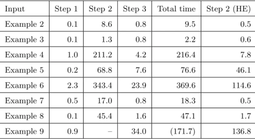
Table 6. Timing data (in seconds)

Input Step 1 Step 2 Step 3 Total time Step 2 (HE)

Example 2 0.1 8.6 0.8 9.5 0.5 Example 3 0.1 1.3 0.8 2.2 0.6 Example 4 1.0 211.2 4.2 216.4 7.8 Example 5 0.2 68.8 7.6 76.6 46.1 Example 6 2.3 343.4 23.9 369.6 114.6 Example 7 0.5 17.0 0.8 18.3 0.5 Example 8 0.1 45.4 1.6 47.1 1.7 Example 9 0.9 – 34.0 (171.7) 136.8

⟨sj+ 1, fj⟩ with a polynomial fj of degree greater than one (j = 3 for Example 2 and j = 2 for Examples 3–6). In the first case,C[x, s]√Υi is obviously prime. It remains to analyse the second case.

We have a ring isomorphism C[x, s]/⟨s1+ 1, fj⟩ ≃ C[x, s2, . . . , sp]/⟨fj⟩. In view of this relation, it is enough to prove that each fj is irreducible over C. For Example 2, f3 = y− x2 is obviously irreducible over C. For Examples 3–6, each f2 has a form

f2= u(x, y) + v(x, y)z with polynomials u(x, y) and v(x, y) in x, y. Since f2 is first order with respect to z, it is reducible over C if and only if u(x, y) and v(x, y) have a non-constant common factor inC[x, y], which is obviously not the case since each v(x, y) is a

monomial. 2

Now that the claim is proved, applying Proposition 4 and Lemma 11 we get, for any α∈ Cn_, Bloc,α(f ) = ∩ i∈σα ((C[x, s]Υi)∩ C[s]) = C[s] · ( ∩ i∈σα (Υi∩ Q[s])),

where σα = {i | 1 ≤ i ≤ r, α ∈ V ((C[x, s]Υi)∩ C[x])}. Notice that by Lemma 11, (C[x, s]Υi)∩ C[x] = C[x](Υi∩ Q[x]). Consequently the computations of Examples 1–6 done overQ are also valid over C. That is, they provide us with stratifications over C such that the local Bernstein-Sato ideal remains the same on each strata.

4. Some remarks on the implementation

Our implementation is realized as a library file “bsi” of Risa/Asir, which will be contained in its distribution (Noro el al.) and/or will be put on the website of the second named author. Table 6 shows the running time (in seconds) of each step of Algorithm 1 on 2.2GHz Intel Core 2 Duo processor with 2GB RAM. In the table, Example 7 is f = (x3 _{+ y}2_{, x}2 _{+ y}3_{), Example 8 is f = (x, x + y}2_{, x + z}2_{), and Example 9 is}

f = (xyz, x3+ y3+ z3). The local Bernstein-Sato ideals for Examples 7, 8, 9 at the origin are principal.

At least for these examples, Step 2 is the most time-consuming part, where the elim-ination is done in one step. Eliminating variables one by one in a suitable order often

speeds up the computation of Step 2 as is shown in the right-most column (HE for heuris-tic elimination) of the table. However, it would be difficult to predict the fastest strategy in advance. Step 1 should be improved by adopting the alternative method of Brian¸con and Maisonobe (2002), as was suggested by Ucha and Castro (2004) and Gago-Vargas et al. (2005). This would require computations in a ring of differential-difference operators, which are not yet available with Risa/Asir.

At the time of this writing, the authors do not know any other systems which are capable of computing local Bernstein-Sato ideals. However, a computer algebra system Singular (Greuel and Pfister (2002)) provides a package “dmod.lib” (Levandovskyy and Morales (2008)) for computing global Bernstein-Sato ideals by the method of Brian¸con and Maisonobe (2002). In our experiments, the performance of our implementation for global Bernstein-Sato ideals is comparable to that of “dmod.lib”.

Acknowledgements

We are grateful to Masayuki Noro for the helpful suggestions on Gr¨obner base compu-tations with Risa/Asir in the ring of differential operators. We would also like to thank the anonymous referees for the constructive comments on the improvement of the present paper.

References

Bahloul, R., 2001. Algorithm for computing Bernstein-Sato ideals associated with a poly-nomial mapping. J. Symbolic Comput. 32, no. 6, 643–662.

Bahloul, R., 2005a. D´emonstration constructive de l’existence de polynˆomes de Bernstein-Sato pour plusieurs fonctions analytiques. Compositio Math. 141, no. 1, 175–191. Bahloul, R., 2005b. Construction d’un ´el´ement remarquable de l’id´eal de Bernstein-Sato

associ´e `a deux courbes planes analytiques. Kyushu J. Math. 59, no. 2, 421–441. Bernstein, J., 1972. Analytic continuation of generalized functions with respect to a

parameter. Funkcional. Anal. i Priloˇzen. 6, no. 4, 26–40.

Brian¸con, J., Maisonnobe, Ph., 2002. Remarques sur l’id´eal de Bernstein associ´e `a des polynˆomes. Preprint Universit´e de Nice Sophia-Antipolis, no. 650.

Brian¸con, J., Maynadier, H., 1999. ´Equations fonctionnelles g´en´eralis´ees : transversalit´e et principalit´e de l’id´eal de Bernstein-Sato. J. Math. Kyoto Univ. 39, no. 2, 215–232. Gago-Vargas, J., Hartillo-Hermoso, M. I., Ucha-Enr´ıquez, J. M., 2005. Comparison of

theoretical complexities of two methods for computing annihilating ideals of polyno-mials, J. Symbolic Comput. 40, no. 3, 1076–1086.

Greuel, G.-M., Pfister, G., 2002. A Singular Introduction to Commutative Algebra. Springer-Verlag, Berlin.

Levandovskyy, V., Martin Morales, J., 2008. Computational D-module theory with Sin-gular, comparison with other systems and two new algorithms. In: Proceedings of the 21st International Symposium on Symbolic and Algebraic Computation, ACM Press, New York, 173–180.

Malgrange, B., 1975. Le polynˆome de Bernstein d’une singularit´e isol´ee. Lecture Notes in Math., pp. 98–119, Vol. 459, Springer, Berlin.

Maynadier, H., 1997. Polynˆomes de Bernstein-Sato asooci´e `a une intersection compl`ete quasi-homog`ene `a singularit´e isol´ee. Bull. Soc. math. France 62, 283–328.

Nakayama, H., 2009. Algorithm computing the local b-function by an approximate divi-sion algorithm in ˆD. J. Symbolic Comput. 44, no. 5, 449–462.

Noro et al. Risa/Asir: an open source general computer algebra system, Developed by Fujitsu Labs LTD, Kobe Distribution by Noro et al., see http://www.math.kobe-u.ac.jp/Asir/index.html.

Oaku, T., 1997a. An algorithm of computing b-functions. Duke Math. J. 87, no. 1, 115– 132.

Oaku, T., 1997b. Algorithms for b-functions, restrictions, and algebraic local cohomology groups of D-modules. Advances in Applied Math. 19, 61–105.

Oaku, T., Takayama, N., 1999. An algorithm for de Rham cohomology groups of the complement of an affine variety via D-module computation. J. Pure Appl. Algebra 139, 201-233.

Sabbah, C., 1987. Proximit´e ´evanescente I. La structure polaire d’unD-Module, Com-positio Math. 62, no. 3, 283–328; Proximit´e ´evanescente II. ´Equations fonctionnelles pour plusieurs fonctions analytiques. Compositio Math. 64, no. 2, 213–241.

Ucha-Enr´ıquez, J. M., Castro-Jim´enez, F. J. , 2004. On the computation of Bernstein-Sato ideals. J. Symbolic Comput. 37, no. 5, 629–639.