Mechanism of Long Transient Oscillations in Cyclic Coupled
Systems
Hiroyuki Kitajima and Yo Horikawa Faculty of Engineering, Kagawa University, 2217-20 Hayashi, Takamatsu, Kagawa, 761-0396 JAPAN
(Dated: June 3, 2009)
Abstract
We consider unidirectionally coupled ring networks of neurons with inhibitory connections. It is known that when a number of inhibitory neurons is even, the system never has stable oscillatory modes. However, we observed oscillatory modes in such a case. In this paper, we clarify the oscillation mechanism in a state space. We investigate the relationship between these oscillatory modes and the unstable periodic solutions(UPSs) generated by the Hopf bifurcations. As a result we find that these transient oscillatory modes are generated by trajectories closing to the UPS and staying around it for a long time. We also confirm this phenomenon in a simple electrical circuit using inverting operational amplifiers.
I. INTRODUCTION
The study on coupled systems is very important as models of information processing in the brain[1], animal locomotion[2], genetic networks[3–5], generating nonlinear phenomena such as chaotic itineracy[6], on-off intermittency[7, 8] and unstable attractors[9, 10], and so on. Moreover, recently we have to treat high-dimensional complex network systems such as small-world[11] and scale-free[12]. In a high-dimensional system, it is very difficult to determine observed complicated phenomenon is transient or steady[13], because transient length becomes large exponentially as a number of cells is increased. Moreover, to clarify its generation mechanism is also very tough, because trajectories, stable and unstable manifolds are not visible in a state space. Thus the analysis of such systems is not enough as far as we know.
In previous studies, we investigated oscillations observed in a unidirectionally coupled neuron model, which is one of high-dimensional systems, with ring structure. It is said that the essential dynamics of some biological central pattern generators can be captured by a model consisting of N neurons connected in ring structure[14–16]. Many investigators con-firm that oscillatory dynamics of neural activity and its synchronization play an important role in information processing in the brain. It is analytically understood that in unidirec-tionally coupled even neurons with inhibitory synapses, the supercritical Hopf bifurcations never occur and attractors are only two equilibrium points[17, 18]. However, we found the existence of oscillatory modes in a system composed of even inhibitory neurons[19, 20].
In this paper, we clarify the oscillation mechanism in a state space. We investigate the relationship between these oscillatory modes and the unstable periodic solutions(UPSs) generated by the Hopf bifurcations. We show that the trajectories corresponding to these oscillatory modes approach the UPS and stay around it for a long time, because the UPS is only one-dimensionally unstable and the unstability is very weak. We also confirm this phenomenon in a simple electrical circuit using inverting operational amplifiers.
II. SYSTEM EQUATION
The system equation of the neuron model is described as
τdxi
where xi is the state of neuron i, n is the number of neurons, τ is the time constant fixed
as 1.0, c is the coupling coefficient and f (x) is the output function given by tan−1(x). This
type of neuron model is commonly used for controlling locomotion [21–23] and describing oscillatory phenomena [18, 24, 25].
We consider c > 0 in Eq. (1), thus Eq. (1) consists of only inhibitory neurons. The system has a stable equilibrium point at the origin for c < 1. The Jacobi matrix of Eq. (1) evaluated at the origin can be written as
C = −In−cPn, (2)
where Inis the identity matrix and Pnis a cyclic matrix. The eigenvalues of C is analytically
obtained as
g(am) = −1 − cam (m = 0, 1, · · · , n − 1), (3) where a = ej2π
n. From Eq. (3), we can see that the eigenvalues are located on the circle
with center (−1,0) and radius c in the complex plane. At c = 1 the pitchfork bifurcation of the equilibrium point occurs and two stable equilibrium points, namely (x1, x2, · · · , xn) =
(A, −A, · · · , −A) and (−A, A, · · · , A), are generated. The eigenvalues of the Jacobi matrix for these equilibrium points are also located on the circle with center (−1,0) and radius c in the complex plane, however the radius becomes smaller as the values of c is increased; this means two equilibrium points are stable for increase of the value of c. When we increase the value of the parameter c again and a pair of the eigenvalues evaluated at the origin becomes pure imaginary numbers, the Hopf bifurcation occurs. Such a value of imaginary numbers indicates an angular frequency of an oscillation generated by the Hopf bifurcation.
III. RESULTS
A. Computer Simulations
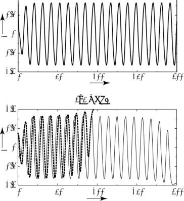
The unstable equilibrium point (the origin) meets several Hopf bifurcations for c > 1. Figure 1(a) shows the waveform of an unstable periodic solution(UPS) generated by the first Hopf bifurcation. This UPS is one-dimensionally unstable, however, stably observed in the invariant subspace xi = −xi+n/2 [20].
Note that for c > 1 only two equilibrium points which are symmetry with respect to the origin are attractors. However, we observe oscillatory modes for sufficiently large n [19]. For
the sake of simplicity, we investigate the mechanism of generating such oscillatory modes for a small number of neurons (n = 12). In this case, although the solutions go to one of quiescence attractors in finite time(Fig. 1(b)), we consider that the mechanism of generating oscillatory modes is the same as the case of large n. The first and second Hopf bifurcations of the origin occur at c ' 1.155 and c ' 2.0, respectively. Thus, we fix the value of c as 1.4 to study the influence of only the first Hopf bifurcation on the oscillatory modes.
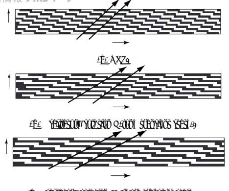
Figure 2(a) shows a temporal pattern for the UPS generated by the Hopf bifurcation. We put initial states as xi = −xi+6 (i = 1, · · · , 6), therefore the UPS is stable in this invariant
subspace. The temporal pattern is symmetrical black and white. From Fig. 2(a) we can see that the switching the signs of state variables occur simultaneously at two neurons and two propagations proceed at the same speed. On the other hand, the temporal black and white patterns of oscillatory modes (Figs. 2(b) and (c)) are asymmetrical and the change of the sign occurs for only one neuron at any time. Finally(the last column in Fig. 2(c)), black and white are alternatively lined. Then the trajectory goes to one of quiescence attractors immediately.
Next, we calculate the sum d of the distance on the sections of xi = 0 (i = 1, 2, · · · , 12).
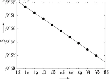
More precisely, when the trajectories cross the sections from a negative value to a positive value, we calculate the Euclidean distance between the oscillatory mode and the UPS and add them for all i. Figure 3 shows the results from four random initial states having a transient oscillation. In every case, the distance is decreased once; this means the solution is close to the UPS. For long transient oscillations(open and closed circles) the trajectories stay around the UPS for a long time, because the UPS is only one-dimensionally unstable. In other words, as the trajectories get closer to the UPS, the transient state or the oscillatory state continues longer.
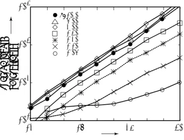
Figure 4 shows the average transient length from 1000 distinct initial states as a function of an even number of neurons. The transient time is exponentially increased as a number of neurons is increased. Because the maximal characteristic multiplier (λ) is closer to one exponentially as n becomes larger (Fig. 5). For increase of the value of c, we can see that decrease of the average transient length is saturated around c = 2.0, because the maximal characteristic multiplier is also saturated around c = 2.0 (Fig. 6). In Fig. 6 we show the average length of transients from 500 random initial states. We can see that the transient time is inverse proportional to the value of the characteristic multiplier. We conclude that
generation of these oscillatory modes is correlated with the UPS and the length of transient is decided by the characteristic multiplier (larger than one) of the UPS.
Kaneko showed similar result on spatio-temporal chaos using chaotic maps[13]. The difference between Kaneko and our study is summarized in Tab. 1. The dynamics of our system is simpler, thus we can clarify the mechanism of generating very long transient states.
B. Circuit Experiment
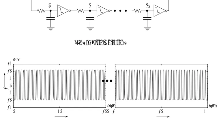
Next, we consider an analog circuit using inverting amplifiers with diffusive coupling, shown in Fig. 7. The output voltage Vout of the inverting amplifiers is a piecewise linear
function of the input voltages Vin as shown in Eq. (4), in which the operating range (the
power supply Vp=12[V]) of the operational amplifiers composing them is taken into account.
Vout = −Vp if Vin> Vp/g, −gVi if −Vp/g ≤ Vin≤Vp/g, Vp if Vin< −Vp/g, (4)
where g = 10 is the gain of the amplifiers. This simple nonlinearity plays an essential role in the stability and transient phenomena of the system. The circuit equation is given by
CRdVi
dt = −Vi+ Vout(Vi−1) (i = 1, · · · , n, V0 ≡Vn). (5) In Eq. (5), the origin is also one of equilibrium points. The Jacobi matrix evaluated at the origin is the same as Eq. (2). Thus bifurcations of the origin occur at the same parameter values of g (Eq. (5)) and c (Eq. (1)). Moreover, the unstable dimension of the generated UPS by the Hopf bifurcations is also the same.
We observe a long transient oscillation shown in Fig. 8, which last more than ten minutes (as a maximum, more than one hour), in the experiment with the circuit of 40 operational amplifiers diffusively coupled with a time constant (RC) 0.1[sec]. A number of nodes and a piecewise linear system are different from those in Sec. IIIA, however the essence is not lost, because the keys of generating this oscillation are even number of nodes and the symmetrical property of inverting state variables
The duration ts of the oscillations approximately obeys a power law distribution, i.e.
f (ts) ' 1/ts, not an exponential distribution. We then study the dependence of the transient
OLIVE 香川大学学術情報リポジトリ
oscillations on fluctuations in the initial values of the voltages of the nodes and variations in the values of the elements with computer simulation. Negative spatial correlations in the initial voltages make the oscillations less occur and shorten the duration, while positive correlations have little effect. Variations in the elements: the resistance R, the capacitance C and the gain g of the amplifiers also decrease the occurrence of the oscillations since they break the symmetry of the system. Long oscillations, however, still appear even though the values of the elements vary in the ranges of the order of several hundred times.
IV. CONCLUSIONS
In this paper, we investigate the mechanism of oscillatory modes in coupled even number of neurons as a ring. In a time domain, these oscillatory modes show switching patterns between positive and negative values. We calculate the distance between the oscillatory modes and the UPS generated by the Hopf bifurcation on the sections xi = 0. This result
shows that these patterns are formed by the trajectories closing to the UPS and staying around it for a long time. We also study the piecewise linear system as the model of an analog circuit. From these results, we consider the key of generating this phenomenon is that the system has the symmetrical property of inverting state variables and two symmetrical equilibrium points with respect to the origin. However, we can say that some perturbations are allowed, because we confirm this phenomenon in a real electrical circuit using inverting operational amplifiers. It is an open problem to study other coupling methods[26, 27] and a system of ring oscillators[28].
[1] N. Katayama, M. Nakao, H. Saitoh, and M. Yamamoto. Dynamics of a hybrid system of a brain neural network and an artificial nonlinear oscillators. BioSystems, 58:249, 2000.
[2] J. J. Collins and I. Stewart. Coupled nonlinear oscillators and the symmetries of animal gaits. J. Nonlinear Science, 3:349, 1993.
[3] K. Horikawa, K. Ishimatsu, E. Yoshimoto, S. Kondo, and H. Takeda. Noise-resistant and synchronized oscillation of segmentation clock. Nature, 441:719, 2006.
[4] C. Li, L. Chen, and K. Aihara. Stochastic synchronization of genetic oscillator networks. BMC Systems Biology, 1(6), 2007.
[5] M.C. Huang, Y.T. Huang, J.W. Wu, and T.S. Chung. Potential for regulatory networks of gene expression near a stable point. arXiv:0710.3837v1, 2007.
[6] Focus issue: Chaotic Itineracy. Chaos, 13(3):926, 2003.
[7] H. Fujisaka and T. Yamada. A new intermittency in coupled dynamical systems. Prog. Theor. Phys., 74(3):918, 1985.
[8] H. Fujisaka and T. Yamada. Stability theory of synchronized motion in coupled-oscillator systems.iv. Prog. Theor. Phys., 75(5):1087, 1986.
[9] C. Kirst and M. Timme. Bifurcation from networks of unstable attractors to heteroclinic switching. arXiv:0709.3432v1, 2007.
[10] P. Ashwin and M. Timme. Unstable attractors: existence and robustness in networks of oscillators with delayed pulse coupling. Nonlinearity, 18:2035, 2005.
[11] D.J. Watts and S.H. Strogatz. Collective dynamics of small-world networks. Nature, 393:440, 1998.
[12] A.L. Barab´asi and R. Albert. Emergence of scaling in random networks. Science, 286:509, 1999.
[13] K. Kaneko. Supertransients, spatiotemporal intermittency and stability of fully developed spatiotemporal chaos. Phys. Lett., 149:105, 1990.
[14] G. B. Ermentrout. The behavior of rings of coupled oscillators. J. Math. Biology, 23:55, 1985. [15] C. C. Canavier, D. A. Baxter, J. W. Clark, and J. H. Byrne. Control of multistability in ring
circuits of oscillators. Biol. Cybern., 80:87, 1999.
[16] C.Y. Park, Y. Hayakawa, K. Nakajima, and Y. Sawada. Limit cycles of one-dimensional neural networks with the cyclic connection matrix. IEICE Trans. Fundamentals, E79-A(6):752, 1996. [17] S. Amari. Mathematics of neural networks. Sangyo-Tosho, 1978 (in Japanese).
[18] Y. Nakamura and H. Kawakami. Bifurcation and chaotic attractor in a neural oscillator with three analog neurons. Electronics and Communications in Japan, 83(9):104, 2000.
[19] T. Ishii and H. Kitajima. Oscillation in cyclic coupled neurons. In Proceedings of Nonlinear Circuit and Signal Processing,, pages 97–100, Honolulu, March 2005.
[20] H. Kitajima, T. Ishii, and T. Hattori. Oscillation mechanism in cyclic coupled neurons. In Proceedings of Nonlinear Theory and its Applications, pages 623–626, Bologna, Sept. 2006. [21] A. Fujii, A. Ishiguro, Y. Uchikawa, T. Aoki, and P. Eggenberger. Gait control for a legged robot
using neural networks with dynamically-rearranging function. IEEJ Trans., 119-C(12):1567,
1999 (in Japanese).
[22] H. Nagashino, M. Kataoka, and Y. Kinouchi. A coupled neural oscillator model for recruitment and annihilation of the degrees of freedom of oscillatory movements. Neurocomputing, 26-27:455, 1999.
[23] H. Nagashino, Y. Nomura, and Y. Kinouchi. A neural network model for quadruped gait generation and transitions. Neurocomputing, 38-40:1469, 2001.
[24] H. H. Yang. Some results on the oscillation of neural networks. In Proceedings of Nonlinear Theory and its Applications, pages 239–242, Las Vegas, Nov. 1995.
[25] K. Jinno and T. Saito. Analysis and synthesis of continuous-time hysteretic neural networks. IEICE Trans. Fundamentals, J75-A(3):552, 1992.
[26] G. N. Borisyuk, R. M. Borisyuk, A. I. Khibnik, and D. Roose. Dynamics and bifurcation of two coupled neural oscillators with different connection types. Bull. Math. Biol., 57(6):809, 1995.
[27] D.J. Watts. Six Degrees: The Science of a Connected Age. W.W. Norton & Company, 2003. [28] H. Tanaka, A. Hasegawa, H. Mizuno, and T. Endo. Synchronizability of distributed clock
-1.2 -0.6 0 0.6 1.2 0 50 100 150 200
t
x
1 (a) UPS. -1.2 -0.6 0 0.6 1.2 0 50 100 150 200t
x
1(b) Short(dashed curve) and long(solid curve) transient oscillatory modes from different initial states.
FIG. 1: (a)Waveforms of UPS and (b)transient oscillatory modes observed in Eq. (1) for n = 12 and c = 1.4.
t
x
i(a) UPS.
t
x
i(b) Oscillatory solution I (long transient state).
t
x
i(c) Oscillatory solution II (short transient state).
FIG. 2: Temporal switching patterns for c = 1.4 and n = 12 in Eq. (1). When the sign of xi is
changed, we put black and white for negative and positive values of xi, respectively. The arrows
0 20 40 60 80 0 50 100 150 200
t
d
FIG. 3: Sum of distance between oscillatory modes and UPS on the every section of xi = 0
(i = 1, · · · , 12). Interval of symbols is almost the same as the period of UPS.
104 103 102 101 12 18 24 30
n
average length of transients
1.05 1.10 1.20 1.30 2.00 5.00 c=10.0
FIG. 4: Average length of transient as a function of a number of neurons.
1e-06 1e-05 1e-04 1e-03 1e-02 1e-01 20 24 28 32 36 40 44 48 52 56 60
λ−1
n
FIG. 5: Maximal eigenvalue as a function of a number of neurons.
c
5.010 4.0 3.0 2.0 1.0 0.0λ−1
-2 101 102 103 104average length of transients
1.0 2.0 3.0
right
left
FIG. 6: Maximal characteristic multiplier(left axis) and average length of transients(right axis) as a function of coupling coefficient c (n=24).
TABLE I: Comparison between results of Kaneko [13] and this model.
system transient state attractor
Kaneko[13] discrete chaotic periodic
this model continuous periodic equilibrium
R C V 1 R C V 2 R C Vn
FIG. 7: Circuit diagram.
-15 -10 -5 0 5 10 15 0 50 100
![TABLE I: Comparison between results of Kaneko [13] and this model.](https://thumb-ap.123doks.com/thumbv2/123deta/5734091.1020025/13.918.112.812.74.181/table-i-comparison-results-kaneko-model.webp)