OPTICAL TECHNOLOGY FOR
ARBITRARILY MANIPULATING
AMPLITUDES AND PHASES OF
HIGHLY DISCRETE SPECTRA
CHUAN ZHANG
THE UNIVERSITY OF ELECTRO-COMMUNICATIONS
TOKYO, JAPAN
OPTICAL TECHNOLOGY FOR
ARBITRARILY MANIPULATING
AMPLITUDES AND PHASES OF
HIGHLY DISCRETE SPECTRA
by
Chuan ZHANG
A thesis submitted in partial fulfillment of the requirements for the degree of Doctor of Philosophy
to
Department of Engineering Science
Graduate School of Informatics and Engineering The University of Electro-Communications
Chofu, Tokyo, Japan January 2020
Copyright c
2020 Chuan ZHANG
Dedicated to my parents
“Physics has a history of synthesizing many
phenomena into a few theories.”
Acknowledgements
I just can not believe how time has flied by! I would like to, hereby, grab the precious opportunity to acknowledge those who have helped me tremendously throughout my PhD career.
First and foremost, I would like to thank my supervisor, Prof. Masayuki Katsuragawa, for his thoughtful care and professional instructions all across my PhD life in UEC. It is his excellent research capability and generous dedi-cation that lead to the accomplishment of my PhD degree.
I appreciate Prof. Kaoru Minoshima, and Prof. Masaru Suzuki for their patient instructions and helpful advices. I thank Yukai Furukawa sensei for his longtime assistance in whatever conducting experiments or analyzing the-ories.
I feel fairly grateful for Dr. Kazumi Yoshii and Dr. Chiaki Ohae on their constructive advices during my research work. I also acknowledge Dr. Jian Zheng, Dr. Nurul Sheeda Binti Suhaimi, and Dr. Trivikramarao Gavara for their selfless help in my PhD life. I, especially, appreciate Dmitry Trigubov for the period of time when we cooperated and moved forward together in the lab.
I would also like to thank all the other labmates who have literally con-tributed vastly to my happy life in the big family of Katsuragawa lab. Without them, it would be hardly probable for me to make good progress in any aspect. Special thanks also attributing to Weiyong Liu, Yoshisaki Kun, Morimune Kun, Suzuki Kun, Shikanai Kun, Watanabe Kun, et al.
Additionally, I have to thank all my nice friends in UEC, with whom I have promoted my communications, enriched my leisure time, and expanded my horizons. All these things during studying abroad will be memorable and nos-talgic in my life afterwards.
Most importantly, I would like to say a big thank-you to my family for their nothing but great support and encouragement. My parents ever communi-cated with me many many times during the highs and lows of my PhD career.
Abstract
This thesis reports a novel optical technology that enables us to arbitrarily manipulate amplitudes and phases of highly discrete broadband spectra. The novel optical technology is concise: we simply place a few fundamental optical elements–a waveplate, a polarizer, and a transparent dispersive plate–on an optical axis and precisely control their thicknesses. However, such optical tech-nology is practically useful: 1, excellent maintenance of beam quality and spa-tial coherence, as it can arbitrarily manipulate amplitudes and phases of any highly discrete (several tens of terahertz) spectrum without separating indi-vidual components in space; 2, resistance to high power lasers, as transparent materials with high damage thresholds are used for transmitting ultrabroad spectra (mid-infrared, visible, and ultraviolet).
We experimentally demonstrate the novel optical technology by manipulat-ing amplitudes and phases of a series of vibrational Raman coherence, which has a frequency spacing of about 125 terahertz and a bandwidth of over 700 terahertz. Specifically, we have succeeded consecutively in manipulating the amplitudes and phases of five (spanning 2,403 to 481 nm), six (spanning 2,403 to 401 nm), and seven (spanning 2,403 to 343 nm) Raman components. Lim-ited by the range of measuring phases of broader spectrum via spectral phase inteferometry, the current system can not handle eight or more Raman com-ponents.
As a typical application of such optical technology, we also demonstrate gen-eration of ultrashort pulses in the time domain, through reconstructing elec-tric field intensity waveforms of the Raman coherence after manipulating its amplitudes and phases. With the aforementioned five Raman components ma-nipulated, we have achieved a train of 1.6 femtosecond (at full width at half maximum) pulses with a repetition rate of about 125 terahertz, close to Fourier transform limited condition. With six Raman components, we have achieved a train of 1.4 femtosecond ultrafast pulses. And finally with seven Raman components, we have achieved a train of 1.2 femtosecond ultrafast pulses.
Table of Contents
1 Introduction 1
1.1 Literature overview and motivation . . . 1
1.1.1 Literature overview . . . 1
1.1.2 The motivation of our work . . . 3
1.2 Thesis overview . . . 6
2 Conceptual idea of the novel optical technology 14 2.1 Conceptual idea of amplitude manipulation . . . 16
2.2 Conceptual idea of phase manipulation . . . 18
2.3 Principle of SPIDER system . . . 24
3 Experimental system 30 3.1 Raman generation . . . 31
3.2 Manipulation devices . . . 33
3.3 SPIDER system . . . 34
TABLE OF CONTENTS
4.1 Photos of Raman components . . . 38
4.2 Results of amplitude manipulation . . . 40
4.2.1 Results of amplitude manipulation of five Raman compo-nents . . . 40
4.2.2 Results of amplitude manipulation of six Raman compo-nents . . . 45
4.2.3 Results of amplitude manipulation of seven Raman com-ponents . . . 48
4.3 Results of phase manipulation . . . 51
4.3.1 Results of phase manipulation of five Raman components 52
4.3.2 Results of phase manipulation of six Raman components 58
4.3.3 Results of phase manipulation of seven Raman components 62
4.4 Electric field intensity waveforms . . . 67
4.4.1 Electric field intensity waveforms achieved with five Ra-man components . . . 68
4.4.2 Electric field intensity waveforms achieved with six Ra-man components . . . 69
4.4.3 Electric field intensity waveforms achieved with seven Ra-man components . . . 71
4.4.4 Electric field intensity waveforms predicted with eight Raman components . . . 73
5 Discussions 76
5.1 Discussions in amplitude manipulation . . . 76
TABLE OF CONTENTS
5.3 Discussions in reconstructing electric field intensity waveforms 91
6 Conclusions and prospects 95
6.1 Conclusions . . . 95
6.2 Prospects . . . 96
Appendix 99
List of Figures
1.1 Key optical technologies open the doors to new optical sciences . 2
1.2 Experimental setup of OAWG techniques and the results of
line-by-line shaping of 108 lines . . . 3
1.3 Schematic diagram of the field synthesis experiments conducted by Han S. Chan, et al. . . 4
2.1 Conceptual idea of manipulating amplitudes and phases of mul-tiple components . . . 15
2.2 Schematic diagram of SPIDER system . . . 25
2.3 Mechanism of retrieving phases of a spectrum with six compo-nents in SPIDER system . . . 26
3.1 The main experimental system . . . 30
3.2 Beam profiles of two driving lasers . . . 31
3.3 Pulse envelopes of two driving lasers . . . 32
3.4 The devices of amplitude and phase manipulations . . . 33
4.1 Photos of Raman components . . . 38
LIST OF FIGURES
4.3 Results of amplitude manipulation of five Raman components . 41
4.4 Results of amplitude manipulation of six Raman components . 46
4.5 Results of amplitude manipulation of seven Raman components 49
4.6 Results of phase manipulation of five Raman components . . . . 52
4.7 Intensities of interfered SFG components illustrated in spectrom-eter . . . 54
4.8 Results of phase manipulation of six Raman components . . . . 59
4.9 Results of phase manipulation of seven Raman components . . 64
4.10 Retrieved electric field intensity waveforms of five high-order Raman components . . . 68
4.11 Retrieved electric field intensity waveforms of six high-order Ra-man components . . . 70
4.12 Retrieved electric field intensity waveforms of seven high-order Raman components . . . 72
4.13 Calculated electric field intensity waveforms of eight high-order Raman components . . . 73
5.1 Acceptance angles of 10 µm thick BBO crystal . . . 87
5.2 Acceptance angles of 5 µm thick BBO crystal . . . 89
List of Tables
5.1 Precision of fitting lines of initial scanning in MA . . . 78
5.2 Comparison of periods of power oscillations between experimen-tal results and theoretical calculation. . . 79
5.3 Precision of achieved power distribution of MA . . . 80
5.4 Comparison of different powers . . . 81
5.5 Precision of fitting lines of intensity oscillations of interfered SFG components . . . 84
5.6 Difference of pulse width due to change of power distributions between MA and MP . . . 92
Chapter 1
Introduction
1.1
Literature overview and motivation
1.1.1
Literature overview
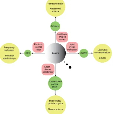
Development of new optical technology always paves the way for the essential evolution of optical science. A handful of typical examples can be enumerated as below (also refer to figure 1.1).
In the time domain, the advent of dielectric multilayer chirped mirrors [1– 3] offered solutions for spectral broadband dispersion control [4, 5], and thus enabled practical solid state femtosecond lasers [6–8]. Benefiting from ultra-high temporal resolution, mode-locked [9–11] femtosecond lasers [12–14] have ever allowed researchers to probe fast-evolving phenomena, such as chemical reactions at the molecular level [15, 16], and further spawned femtochemistry [17] (for which Ahmed Zewail was awarded the Nobel Prize for Chemistry in 1999) and attosecond science [18–20].
In the frequency domain, the use of photonic crystal fiber (PCF) [21–23] for spectral bandwidth broadening permitted self-referencing method to mea-sure carrier envelope offset (CEO) frequency, thus advanced optical frequency comb (OFC) [24, 25]. With the capability of measuring absolute optical
fre-1.1. LITERATURE OVERVIEW AND MOTIVATION
quencies, OFC technology (for which John L. Hall and Theodor W. Hansch were awarded the Nobel Prize for Physics in 2005) has revolutionized optical frequency metrology [26] and precision spectroscopy [27].
Figure 1.1: Key optical technologies open the doors for new optical sciences.
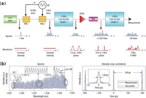
In addition, dominated by liquid crystal modulators (LCM) [28, 29], optical arbitrary waveform generation (OAWG) [30, 31] techniques (see figure 1.2) pro-vided a means of controlling spectral intensities and phases of optical waves, and synthesizing arbitrary optical waveforms. Combining optical frequency comb with pulse shaping, OAWG technology has the advantages to be widely applied to lightwave communications [32], light detection and ranging (LI-DAR) [31, 33], etc.
1.1. LITERATURE OVERVIEW AND MOTIVATION
Figure 1.2: Experimental setup of OAWG techniques and the results of line-by-line shaping of 108 lines. (a), Schematic diagram. (b), Spectrum and inten-sity cross-correlation for the selected 108 lines at the exit. DDF: dispersion-decreasing fiber; RF: radio frequency; EDFA: erbium-doped fiber amplifier. [Courtesy of Nature Photonics 1, 463 (2007).] [34]
Although in an interdisciplinary way, by using high intensity lasers to inter-act with matters to produce a plasma ambience, such as protons and ions, the adoption of laser plasma accelerators enabled the acceleration of lighter parti-cles such as electrons and positrons, thus making laser-driven particle beams [35]. With the unique characteristics of high energy and high quality, laser driven particle beams are expected to be useful in a wide range of contexts, in-cluding high energy particle physics, plasma science, medical treatment, etc.
1.1.2
The motivation of our work
Launched in the beginning of the 21st century, attosecond pulses [36–38] have been one of the most prominent frontiers in optical science [39–44], and have led the trend of exploring ever fast-evolving events [45–47] at an atomic scale.
1.1. LITERATURE OVERVIEW AND MOTIVATION
Figure 1.3: Schematic diagram of the field synthesis experiments conducted by Han S. Chan, et al. (a), Schematic diagram of the experimental setup to synthesize waveforms using harmonics generated by coherent modulation of the H2molecules. AM and PM are liquid crystal spatial light modulators
(LC-SLMs) that, respectively, attenuate the powers (and thus amplitudes) of the harmonics, and adjust and compensate their phases; and these two abbrevi-ations are only used here. These LCSLMs are also used as pulse shapers for the cross-correlation measurements. (b), Pictorial demonstration of ultrafast waveforms obtained by the coherent superposition of the first five harmonics of a fundamental wavelength. The panel on the lower right depicts the spec-tral field amplitudes required for the synthesis of the respective waveforms on the left. The 8.02-fs pulse spacing originates from a fundamental wavelength of 2,406 nm. [Courtesy of Science 331, 1165 (2011).] [48]
On the other hand, Stephen E. Harris and collaborators [49–52] provided a way of generating sub-femtosecond pulses via molecular modulation [53, 54] in the 1990s. A. H. Kung and others [48] experimentally verified to manipulate amplitudes and phases of five discrete Raman components and were able to synthesize arbitrary optical waveforms (see figure 1.3).
1.1. LITERATURE OVERVIEW AND MOTIVATION
Motivated by the above backdrops, we expected to experimentally combine the techniques of synthesizing optical waveforms (pulse shaping in a broad sense), with a highly discrete Raman coherence (an optical frequency comb in a broad sense) to approach attosecond pulses in the time domain. Note that this discrete spectrum of Raman coherence is produced by molecular modu-lation process, not through high harmonic generation [55–57] that can yield ultrashort pulses with a pulse duration of several tens of attoseconds (scatter-ing extreme ultra violet or soft X rays [58–60]),
In this thesis, I report a novel optical technology, which allows us to arbitrar-ily manipulate amplitudes and phases of highly discrete broadband spectra. The optical technology is simple, that is, we just place a few fundamental opti-cal elements–a waveplate, a polarizer, and a transparent dispersive plate–on an optical axis and precisely control their thicknesses.
In spite of its simplicity, the novel optical technology is very powerful. Un-like line-by-line shapers [61, 62] used in OAWG techniques, we do not spatially separate the optical waves to control spectral components individually (such case can also be found in figure 1.3). Therefore, one of the attractive advan-tages is that the manipulation devices maintain excellent spatial coherence of the optical waves. Moreover, the manipulation devices are very robust to resist high energy laser radiations, as we exploit transparent materials that all have high damage thresholds.
We have, so far, applied our manipulation devices to harness the amplitudes and phases of five, six, and seven adiabatically driven vibrational Raman com-ponents (with a frequency spacing of about 125 THz) in sequence. With the broadest Raman spectrum–seven modes (covering 2,403 to 343 nm, with a bandwidth of over 700 terahertz)–handled, we have achieved a train of 1.2 femtosecond (at full width at half maximum) single-cycle pulses in the time domain, with a repetition period of about 8 femtoseconds.
In recent years, researchers have experimentally demonstrated optical field-induced changes in dielectric materials, namely, that the physical properties of dielectrics can be changed by controlling optical fields [63–65] on sub-femtosecond to few-femtosecond timescales. As a potential application regarding high speed
1.2. THESIS OVERVIEW
information processing, in terms of light-to-light, the trains of ultrafast pulses we achieved may become a key tool in this field. Considering that researches on ultrafast optics have been continuously flourishing, more applications are about to be discovered.
1.2
Thesis overview
As narrated partly in the abstract, this thesis accounts for the proposal, theo-retical analysis, and experimental demonstration of a novel optical technology– arbitrary manipulation of amplitudes and phases of highly discrete spectra. Through Fourier transform of the manipulated spectra, we are also able to reconstruct electric field intensity waveforms, which are trains of ultrashort pulses in the time domain. Below shows detailed contents of each chapter.
Chapter 2 conceptually illustrates the idea of amplitude manipulation, and
phase manipulation, respectively. In particular, this chapter shows why the novel optical technology is eligible for manipulating amplitudes and phases of multi-frequencies, and the advantages of such optical technology.
Chapter 3 introduces the entire experimental system, which mainly
en-compasses three parts: generation of Raman coherence, amplitude and phase manipulations, and phase measurement.
The first part of the system yields the laser source for use, i.e., a highly dis-crete broadband spectrum. Afterwards, the second part is the core content of the novel optical technology–amplitude and phase manipulations. Finally, the third part introduces phase measurement through spectral phase inter-ferometry, which is the difficult point of the whole system since its precision and limitation substantially affect the viability and development of such novel optical technology.
Chapter 4 shows the main results experimentally obtained. In section 4.1,
I will show the actual photos of Raman components generated. In section 4.2, I will show the results of amplitude manipulation in detail. And in section 4.3, I will show the results of phase manipulation. As we have manipulated
1.2. THESIS OVERVIEW
amplitudes and phases of different number of Raman components, I will ex-hibit the results sequentially, namely, begin with the results of five, then to six, and eventually to seven Raman modes. As a typical application of our manipulation devices, in section 4.4, I will also show reconstruction of electric field intensity waveforms of different number of Raman components, which are trains of ultrashort pulses in the time domain.
Chapter 5 concentrates on the main issues discussed during the process
of manipulating amplitudes and phases of different number of Raman modes. Especially, I will explain the difficulties of increasing the number of Raman modes for both amplitude and phase manipulations, the precision estimated, the differences of pulses following the escalation of the number of Raman modes, the limitations of the current system, etc.
Chapter 6 summarizes the whole work in the thesis. Afterwards, this
chap-ter gives prospects for future research, and examplifies potential applications of our novel optical technology, including its achievement of ultrashort pulses.
Bibliography of Chapter 1
[1] F. X. Kartner et al. “Design and fabrication of double-chirped mirrors”. In: Opt. Lett. 22 (1997), pp. 831–833.
[2] R. Szipocs and A. K. Kis. “Theory and design of chirped dielectric laser mirrors”. In: Appl. Phys. B 65 (1997), pp. 115–135.
[3] N. Matuschek, F. X. Kartner, and U. Keller. “Theory of double-chirped mirrors”. In: IEEE J. of Selected Topics In Quant. Elect. 4 (1998), pp. 197– 208.
[4] R. Szipocs et al. “Chirped multilayer coatings for broadband dispersion control in femtosecond lasers”. In: Opt. Lett. 19 (1994), pp. 201–203. [5] N. Matuschek et al. “Back-side-coated chirped mirrors with ultra-smooth
broadband dispersion characteristics”. In: Appl. Phys. B 71 (2000), pp. 509– 522.
[6] A. Stingl et al. “Sub-10-fs mirror-dispersion-controlled Ti:sapphire laser”. In: Opt. Lett. 20 (1995), pp. 602–604.
[7] E. J. Mayer et al. “Ultrabroadband chirped mirrors for femtosecond lasers”. In: Opt. Lett. 22 (1997), pp. 528–530.
[8] V. Pervak et al. “High-dispersive mirrors for femtosecond lasers”. In:
Opt. Express16 (2008), pp. 10220–10232.
[9] E. P. Ippen. “Principles of passive mode locking”. In: Appl. Phys. B 58 (1994), pp. 159–170.
[10] S. T. Cundiff, J. Ye, and J. L. Hall. “Optical frequency synthesis based on mode-locked lasers”. In: Rev. of Sci. Inst. 72 (2001), pp. 3749–3771.
BIBLIOGRAPHY OF CHAPTER 1
[11] A. Bartels, D. Heinecke, and S. A. Diddams. “Passively mode-locked 10 GHz femtosecond Ti:sapphire laser”. In: Opt. Lett. 33 (2008), pp. 1905– 1907.
[12] U. Morgner et al. “Sub-two-cycle pulses from a Kerr-lens mode-locked Ti:sapphire laser”. In: Opt. Lett. 24 (1999), pp. 920–922.
[13] L. Gallmann et al. “Characterization of sub-6-fs optical pulses with spec-tral phase interferometry for direct electric-field reconstruction”. In: Opt.
Lett.24 (1999), pp. 1314–1316.
[14] M. Miranda et al. “Simultaneous compression and characterization of ultrashort laser pulses using chirped mirrors and glass wedges”. In: Opt.
Express20 (2012), pp. 688–697.
[15] M. Shapiro and P. Brumer. “Coherent control of molecular dynamics”. In: Rep. Prog. Phys. 66 (2003), pp. 859–942.
[16] C. Brif, R. Chakrabarti, and H. Rabitz. “Control of quantum phenomena: Past, present and future”. In: New J. Phys. 12 (2010), p. 075008.
[17] A. H. Zewail. “Femtochemistry: atomic-scale dynamics of the chemical bond”. In: J. Phys. Chem. A 104 (2000), pp. 5660–5694.
[18] M. Hentschel et al. “Attosecond metrology”. In: Nature 414 (2001), pp. 509– 513.
[19] P. B. Corkum and F. Krausz. “Attosecond science”. In: Nat. Phys. 3 (2007), pp. 381–387.
[20] F. Krausz and M. K. Stockman. “Attosecond metrology: from electron capture to future signal processing”. In: Nat. Photon. 8 (2014), pp. 205– 213.
[21] J. C. Knight et al. “All-silica single-mode optical fiber with photonic crys-tal cladding”. In: Opt. Lett. 21 (1996), pp. 1547–1549.
[22] T. A. Birks, J. C. Knight, and P. S. J. Russell. “Endlessly single-mode photonic crystal fiber”. In: Opt. Lett. 22 (1997), pp. 961–964.
[23] J. C. Knight. “Photonic crystal fibers”. In: Nature 424 (2003), pp. 847– 851.
BIBLIOGRAPHY OF CHAPTER 1
[24] T. Udem et al. “Absolute optical frequency measurement of the cesium D1 line with a mode-locked laser”. In: Phys. Rev. Lett. 82 (1999), pp. 3568– 3571.
[25] D. J. Jones et al. “Carrier-envelope phase control of femtosecond mode-locked lasers and direct optical frequency synthesis”. In: Science 288 (2000), pp. 635–639.
[26] T. Udem, R. Holzwarth, and T. W. Hansch. “Optical frequency metrol-ogy”. In: Nature 416 (2002), pp. 233–237.
[27] R. Holzwarth et al. “Optical frequency synthesizer for precision spec-troscopy”. In: Phys. Rev. Lett. 85 (2000), pp. 2264–2267.
[28] A. M. Weiner et al. “Programmable shaping of femtosecond pulses by use of a 128-element liquid-crystal phase modulator”. In: IEEE J. Quant.
Electron.28 (1992), pp. 908–920.
[29] M. M. Wefers and K. A. Nelson. “Generation of high-fidelity programmable ultrafast optical waveforms”. In: Opt. Lett. 20 (1995), pp. 1047–1049. [30] Z. Jiang, D. E. Leaird, and A. M. Weiner. “Line-by-line pulse shaping
control for optical arbitrary waveform generation”. In: Opt. Express 13 (2005), pp. 10431–10439.
[31] A. M. Weiner. “Ultrafast optical pulse shaping: a tutorial review”. In:
Opt. Comm.284 (2011), pp. 3669–3692.
[32] D. J. Geisler et al. “Modulation-format agile, reconfigurable Tb/s trans-mitter based on optical arbitrary waveform generation”. In: Opt. Express 17 (2009), pp. 15911–15925.
[33] S. T. Cundiff and A. M. Weiner. “Optical arbitrary waveform generation”. In: Nat. Photon. 4 (2010), pp. 760–766.
[34] Z. Jiang et al. “Optical arbitrary waveform processing of more than 100 spectral comb lines”. In: Nat. Photon. 1 (2007), pp. 463–467.
[35] v. Malka et al. “Principles and applications of compact laser–plasma ac-celerators”. In: Nat. Phys. 4 (2008), pp. 447–453.
[36] J. Itatani et al. “Attosecond streak camera”. In: Phys. Rev. Lett. 88 (2002), p. 173903.
BIBLIOGRAPHY OF CHAPTER 1
[37] M. Kitzler et al. “Quantum theory of attosecond XUV pulse measure-ment by laser dressed photoionization”. In: Phys. Rev. Lett. 88 (2002), p. 173904.
[38] E. Goulielmakis et al. “Attosecond control and measurement: lightwave electronics”. In: Science 317 (2007), pp. 769–775.
[39] A. L. Schawlow and C. H. Townes. “Infrared and optical masers”. In:
Phys. Rev.112 (1958), pp. 1940–1949.
[40] T. H. Maiman. “Stimulated optical radiation in ruby”. In: Nature 187 (1960), pp. 493–494.
[41] P. A. Franken et al. “Generation of optical harmonics”. In: Phys. Rev.
Lett.7 (1961), pp. 118–119.
[42] J. A. Armstrong et al. “Interactions between light waves in a nonlinear dielectric”. In: Phys. Rev. 127 (1962), pp. 1918–1939.
[43] R. L. Fork et al. “Compression of optical pulses to six femtoseconds by using cubic phase compensation”. In: Opt. Lett. 12 (1987), pp. 483–485. [44] J. C. Diels and W. Rudolph. “Compression of high-power optical pulses”.
In: J. Opt. Soc. Am. B 5 (1988), pp. 641–647.
[45] T. L. Cocker et al. “Tracking the ultrafast motion of a single molecule by femtosecond orbital imaging”. In: Nature 539 (2016), pp. 263–267. [46] A. Baltuska et al. “Attosecond control of electronic processes by intense
light fields”. In: Nature 421 (2003), pp. 611–615.
[47] A. Sommer et al. “Attosecond nonlinear polarization and light–matter energy transfer in solids”. In: Nature 534 (2016), pp. 86–90.
[48] H. S. Chan and others. “Synthesis and measurement of ultrafast wave-forms from five discrete optical harmonics”. In: Science 331 (2011), pp. 1165– 1168.
[49] S. E. Harris and A. V. Sokolov. “Subfemtosecond pulse generation by molecular modulation”. In: Phys. Rev. Lett. 81 (1998), pp. 2894–2897. [50] A. V. Sokolov, D. D. Yavuz, and S. E. Harris. “Subfemtosecond pulse
generation by rotational molecular modulation”. In: Opt. Lett. 24 (1999), pp. 557–559.
BIBLIOGRAPHY OF CHAPTER 1
[51] A. V. Sokolov et al. “Generation and control of femtosecond pulses by molecular modulation”. In: J. of Mod. Opt. 52 (2005), pp. 285–304. [52] M. Y. Shverdin et al. “Generation of a single-cycle optical pulse”. In: Phys.
Rev. Lett.94 (2005), p. 033904.
[53] N. Zhavoronkov and G. Korn. “Generation of single intense short optical pulses by ultrafast molecular phase modulation”. In: Phys. Rev. Lett. 88 (2002), p. 203901.
[54] S. Baker et al. “Femtosecond to attosecond light pulses from a molecular modulator”. In: Nat. Photon. 5 (2011), pp. 664–671.
[55] J. J. Macklin, J. D. Kmetec, and C. L. III Gordon. “High-order harmonic generation using intense femtosecond pulses”. In: Phys. Rev. Lett. 70 (1993), pp. 766–769.
[56] A. L’Huillier and P. Balcou. “High-order harmonic generation in rare gases with a 1-ps 1053-nm laser”. In: Phys. Rev. Lett. 70 (1993), pp. 774– 777.
[57] C. Altucci et al. “Influence of atomic density in high-order harmonic gen-eration”. In: J. Opt. Soc. Am. B 13 (1996), pp. 148–156.
[58] P. Sali´eres et al. “Frequency-domain interferometry in the XUV with high-order harmonics”. In: Phys. Rev. Lett. 83 (1999), pp. 5483–5486. [59] Y. Mairesse et al. “Attosecond synchronization of high-harmonic soft
x-rays”. In: Science 302 (2003), pp. 1540–1543.
[60] N. Dudovich et al. “Measuring and controlling the birth of attosecond XUV pulses”. In: Nat. Phys. 2 (2006), pp. 781–786.
[61] K. R. Pandiri et al. “Line-by-line control of 10-THz-frequency-spacing Raman sidebands”. In: Opt. Express 18 (2010), pp. 732–739.
[62] K. R. Pandiri and M. Katsuragawa. “A 10 THz ultrafast function generator-generation of rectangular and triangular pulse trains”. In: New J. Phys. 13 (2011), p. 023030.
[63] A. Schiffrin et al. “Optical- field-induced current in dielectrics”. In:
Sci-ence493 (2013), pp. 70–74.
[64] M. Schultze et al. “Controlling dielectrics with the electric field of light”. In: Nature 493 (2013), pp. 75–78.
BIBLIOGRAPHY OF CHAPTER 1
[65] T. Rybka et al. “Sub-cycle optical phase control of nanotunnelling in the single-electron regime”. In: Nat. Photon. 10 (2016), pp. 667–670.
Chapter 2
Conceptual idea of the novel
optical technology
In this chapter, I will illustrate conceptual idea of the novel optical technology– amplitude and phase manipulations.
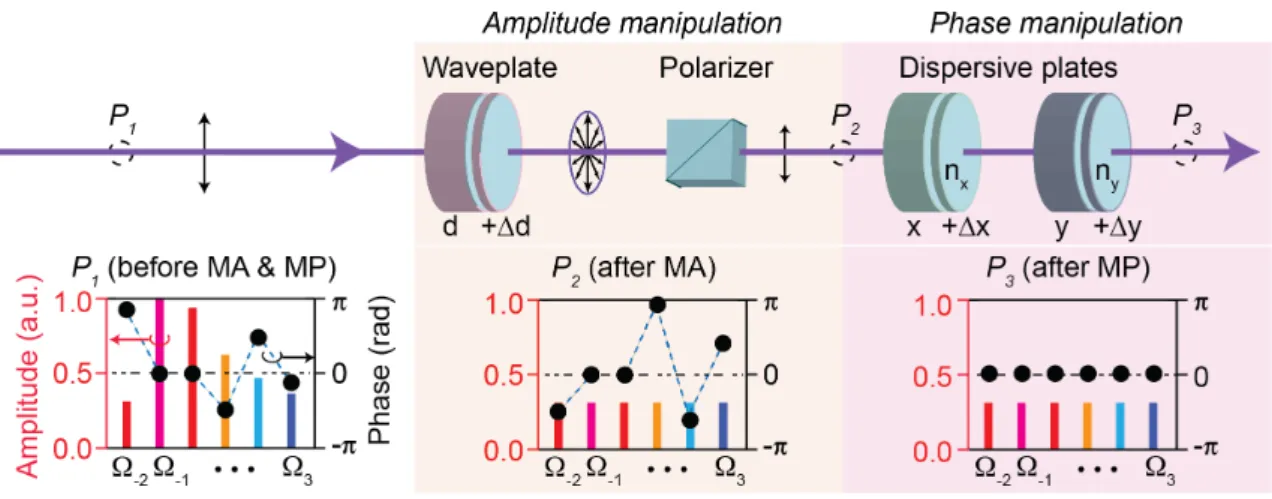
The idea of the novel optical technology is very realistic: we have already been able to control an optical wave with a single frequency flexibly, whether in terms of its amplitude, or phase. In detail, we can exploit an anisotropic ma-terial (waveplate in a broad sense) and a polarizer to control the polarization direction and intensity (thus amplitude) of output laser (i.e., manipulation of amplitude, MA); and utilize a transparent dispersive plate to control the phase of transmitted laser (i.e., manipulation of phase, MP). These are basic optical principles. However, what if the incident optical wave has a broad spectrum with several discrete frequencies, especially, some peculiar spectrum resem-bling vibrational Raman coherence (with a large frequency spacing)? Can we still arbitrarily manipulate amplitudes and phases of such broad spectrum? The answer to this question is affirmative. That is, we can imitate the case of controlling amplitude and phase of a monochromatic laser, to control ampli-tudes and phases of a broad discrete spectrum with a large frequency spacing.
Figure 2.1: Conceptual idea of manipulating amplitudes and phases of mul-tiple components. Without loss of generality, we put the number of spectral components to six. Note that the diagram shows a top view of such idea. P1,
P2, and P3 correspond to different positions on the optical axis, which are
be-fore manipulating amplitudes (MA), after MA, and after manipulating phases (MP), respectively. Bidirectional-black arrows and the ellipse behind the wave-plate represent polarization states at respective positions; d + ∆d, x + ∆x, and y + ∆yare adjustable thicknesses of different plates; nx and ny are refractive
indices of the two dispersive plates; Ω−2–Ω3 are frequencies of different
com-ponents.
Figure 2.1 shows the conceptual idea of arbitrary manipulation on ampli-tudes and phases. The middle part (light yellow background) depicts compact setup for MA, and the rightmost part (pink background) depicts setup for MP. See the next two sections for details.
Afterwards, I will show the principle of SPIDER system, which was used for measuring phases of highly discrete spectra.
These three sections make up core contents of theory of the novel optical technology.
2.1. CONCEPTUAL IDEA OF AMPLITUDE MANIPULATION
2.1
Conceptual idea of amplitude manipulation
The physical mechanism of our amplitude manipulation is by using birefrin-gent property in anisotropic materials. According to the principle of optical birefringence in an anisotropic material [66], the phase retardation between ordinary and extraordinary rays is given by
Γm =
2πΩm
c (nm,e− nm,o)∆d (2.1) where subscript m= -2, -1, ..., indicates mode number of the spectrum; Ωm, nm,e
and nm,o are frequency, refractive indices of the extraordinary, and ordinary
rays in the waveplate, respectively; c is the speed of light in vacuum; and ∆d is thickness change of the waveplate.
To put simply, in experiment, we set the optical axis of the waveplate 45 de-grees to the direction of linear polarization of the incident laser. Taking into account decreasing reflection loss at surfaces of MA and MP elements, we set both the direction of linear polarization of the incident laser and the trans-mission direction of the polarizer to be p-polarized (refer to figure 2.1). With the above settings, laser intensity after transmitting through the polarizer is given as Im = cos2( Γm 2 ) (2.2) or Im = cos2( πΩm c (nm,e− nm,o)∆d) (2.3) which is a sinusoidal function of the thickness change of the waveplate, ∆d, and hence periodical. By varying thickness of the waveplate, we can observe periodical oscillations of intensities at the exit.
What is noteworthy is that the spectrum to be handled should be highly discrete–frequency spacing (∆Ω = Ωm+1 − Ωm) is of several tens of terahertz–
2.1. CONCEPTUAL IDEA OF AMPLITUDE MANIPULATION
so that Ωm (and thus Γm) differs drastically depending on its mode number,
m. In other words, output intensities of various modes oscillate distinctively, in terms of their periods as a function of the thickness of the waveplate. As a result, this makes it feasible to arbitrarily manipulate intensities (or ampli-tudes) of multiple frequencies simultaneously.
Given that the above concept concerns changing the thickness of the plate to realize intensity oscillations, adjustment of the thickness of the wave-plate (actually, both the anisotropic crystal and the transparent dispersive plate) should reach a fine resolution (5 µm) over a wide range (at least 10 mm estimated). Therefore, how we can precisely and handily harness thickness change of the waveplate becomes one of the key points in practical experiment. This issue will be mentioned again and get tackled in the part of experimental system in chapter 3.
Another key point in experiment is that since we expect to manipulate sev-eral amplitudes at the same time, oscillations of different components, con-sidered altogether, are very complicated and even random to some extent. It is hardly possible for us to directly predict or determine an optimal solution, which may be extremely large and unrealistic. Nevertheless, as key physics discovered [67]: when the discreteness (i.e., frequency spacing) of optical spec-trum is high enough (to the order of a few tens of terahertz), we abandon the insistence of exactly finding an analytic solution, but try to find approximate solutions, which frequently appear with sufficient accuracy (more practical in such sense), through numerical exploration. In other words, we will numeri-cally explore an optimal thickness close to the ideal solution (analytic) for ma-nipulating amplitudes (same as the case of mama-nipulating phases), and then validate it in real experiment.
Generally, the more complicated the amplitude distribution we want to achieve is, the more difficult it is to find an optimal thickness through numerical explo-ration. If we want to arbitrarily manipulate amplitudes to any complicated dis-tribution, we should have very wide range of thickness change of crystal quartz for numerical exploration, which is unrealistic. However, since we would like to achieve ultrashort pulses in the time domain, we need to tailor amplitudes of the spectrum to a ‘flat’ distribution, which makes sense that it is a proof of
2.2. CONCEPTUAL IDEA OF PHASE MANIPULATION
our novel optical technology in reality.
Based on the idea of numerical exploration, we desire to manipulate multi-ple intensities at exit of the waveplate. As shown in figure 2.1, before manip-ulating (inset-P1), intensities of various components may be greatly different.
However, using the novel optical technology, ideally we are able to flatten all the intensities/ amplitudes to the same value (inset-P2), which contributes to
generating a train of ultrafast pulses.
2.2
Conceptual idea of phase manipulation
The physical mechanism of our phase manipulation is by using chromatic persion in transparent materials. Based on the principle of chromatic dis-persion, we have to take into account high order dispersions of a broadband spectrum [68] in dispersive materials.
φ(Ωm) = m−1
X
k=0
(Φk∆L(m∆Ω)k) (2.4)
where m represents different spectral components; φ(Ωm)is spectral phase to
be determined; Φk is coefficient of the k-th order dispersion with respect to
φ(Ωm); ∆L is thickness change of the transparent material.
Given a spectrum with m components, the phase, φ(Ωm)should be expanded
up to the k=(m-1)-st order dispersion. In other words, to determine a spectrum with m components, we need to consider its dispersions from the zeroth order up to the (m-1)-st order.
It is noteworthy that the physical mechanism of phase manipulation is sim-ilar to that of amplitude manipulation: depending on component of the highly discrete spectrum, different order dispersion, Φk∆L(m∆Ω)khas largely
differ-ent coefficidiffer-ent, Φk(m∆Ω)k. For example, taking into account fused silica,
coeffi-cients are: Φ2(∆Ω)2= - 1.786 × 10²rad/mm, Φ3(∆Ω)3= 6.664 × 100rad/mm, and
2.2. CONCEPTUAL IDEA OF PHASE MANIPULATION
case of calcium fluoride. By varying thickness of the transparent dispersive material, ∆L, we are able to alter each spectral phase φ(Ωm) independently
and arbitrarily.
Generally, to determine spectral phases exactly in a dispersive material, we have to solve the set of equations as below.
φ(Ωm) = m−1 X k=0 (Φk∆L(m∆Ω)k) = pm+ 2qmπ (2.5) where 0 ≤ pm < 2π; qm is an integer.
As a typical example, if we assume that there are five components, i.e., m = 5, equation 2.5 can be given as:
φ(Ωm) = 4
X
k=0
(Φk∆L(m∆Ω)k) = pm+ 2qmπ (2.6)
Refer to [68]. To simplify notations, we let Φk∆L = Ψk. Thus, the above
equation can be transformed as:
φ(Ω1) = Ψ0+ Ψ1(∆Ω) + Ψ2(∆Ω)2+ Ψ3(∆Ω)3+ Ψ4(∆Ω)4 = p1+ 2q1π φ(Ω2) = Ψ0+ Ψ1(2∆Ω) + Ψ2(2∆Ω)2+ Ψ3(2∆Ω)3+ Ψ4(2∆Ω)4 = p2+ 2q2π φ(Ω3) = Ψ0+ Ψ1(3∆Ω) + Ψ2(3∆Ω)2+ Ψ3(3∆Ω)3+ Ψ4(3∆Ω)4 = p3+ 2q3π φ(Ω4) = Ψ0+ Ψ1(4∆Ω) + Ψ2(4∆Ω)2+ Ψ3(4∆Ω)3+ Ψ4(4∆Ω)4 = p4+ 2q4π φ(Ω5) = Ψ0+ Ψ1(5∆Ω) + Ψ2(5∆Ω)2+ Ψ3(5∆Ω)3+ Ψ4(5∆Ω)4 = p5+ 2q5π (2.7)
2.2. CONCEPTUAL IDEA OF PHASE MANIPULATION Ψ0 = 5(p1+ 2q1π) − 10(p2 + 2q2π) + 10(p3+ 2q3π) − 5(p4+ 2q4π) + (p5+ 2q5π) Ψ1 = 12∆Ω1 (−77(p1 + q1π) + 214(p2 + q2π) − 234(p3 + 2q3π) + 122(p4 + 2q4π) − 25(p5+ 2q5π)) Ψ2 = 24∆Ω1 2(71(p1 + q1π) − 236(p2 + q2π) + 294(p3 + 2q3π) − 164(p4 + 2q4π) + 35(p5+ 2q5π)) Ψ3 = 12∆Ω1 3(−7(p1+q1π)+26(p2+q2π)−36(p3+2q3π)+22(p4+2q4π)−5(p5+2q5π)) Ψ4 = 24∆Ω1 4((p1+ q1π) − 4(p2+ q2π) + 6(p3+ 2q3π) − 4(p4+ 2q4π) + (p5+ 2q5π)) (2.8)
However, since this thesis mainly concerns with generating ultrashort pulses, the zeroth order dispersion, Ψ0, and the first order dispersion, Ψ1, make no
con-tribution to the shape of electric field intensity waveforms (to put it simply, the appearance of pulses), but only change the position (zeroth order) and the lin-ear slope (first order) of intensity waveforms. As a consequence, we can neglect dispersions of the zeroth and first orders.
To further simplify the notation, we make φk = Ψk(∆Ω)k. Therefore,
equa-tion 2.8 can be given as:
φ2 = 1 24(71(p1+q1π)−236(p2+q2π)+294(p3+2q3π)−164(p4+2q4π)+35(p5+2q5π)) = 1 24(2π(71q1− 2 2×59q 2+ 2×3×72q3− 22×41q4+ 5×7q5) + (71p1− 22×59p2+ 2×3×72p3− 22×41p4+ 5×7p5)) = 1 24(2πA + B) (2.9)
2.2. CONCEPTUAL IDEA OF PHASE MANIPULATION
where
A = 71q1− 22×59q2+ 2×3×72q3− 22×41q4+ 5×7q5 (2.10)
B = 71p1− 22×59p2+ 2×3×72p3− 22×41p4+ 5×7p5 (2.11)
Similarly, we can obtain:
φ3 = 1 12(2π(−7q1+ 26q2− 36q3+ 22q4− 5q5) + (−7p1+ 26p2− 36p3+ 22p4− 5p5)) = 1 24(2πC + D) (2.12) where C = −7q1+ 26q2− 36q3+ 22q4− 5q5 (2.13) D = −7p1+ 26p2− 36p3+ 22p4− 5p5 (2.14) And φ4 = 1 24(2π(q1− 4q2+ 6q3 − 4q4+ q5) + (p1− 4p2+ 6p3− 4p4+ p5)) = 1 24(2πE + F ) (2.15) where E = q1− 4q2+ 6q3− 4q4+ q5 (2.16) F = p1 − 4p2+ 6p3 − 4p4+ p5 (2.17)
Since qm is an integer, the term A (or C, E) is also an integer. Therefore,
2.2. CONCEPTUAL IDEA OF PHASE MANIPULATION φ2 = 2π Q2 24 + P2 24 (2.18) φ3 = 2π Q3 12 + P3 12 (2.19) φ4 = 2π Q4 24 + P4 24 (2.20)
where Q2 = 0, 1, ..., 23; Q3 = 0, 1, ..., 11; Q4 = 0, 1, ..., 23; P2, P3, and P4 are
real numbers determined by spectral phases pm. Here, we obtain 24 values of
φ2, 12 values of φ3, and 24 values of φ4.
However, as the relations below exist:
A + C = 2(25q1− 3 × 5 × 7q2+ 3 × 43q3− 71q4+ 3 × 5q5) (2.21)
A + E = 12(23q1− 22× 5q2 + 52q3− 2 × 7q4+ 3q5) (2.22)
C + E = 2(−3q1 + 11q2− 15q3+ 9q4− 2q5) (2.23)
In detail, the sum of A and C is an even integer–Q2 and Q3 are both even
or odd integers–making (24×12)/2 = 144 solutions in the solution space of (φ2,
φ3). Similarly, the sum of A and E is an multiple of 12, making (24×24)/12 =
48 solutions in the solution space of (φ2, φ4). The sum of C and E is an even
integer, also making (24×12)/2 = 144 solutions in the solution space of (φ3, φ4).
Thereby, there are (24×12×24)/(2×12) = 288 solutions in total in the three dimensional solution space, (φ2, φ3, φ4). These many exact solutions make it
easy for us to find near-optimal solutions when manipulating spectral phases of multiple components. The numerous solutions to equation 2.5 features pe-riodical behavior of spectral phase (with a period of 2π).
One might think of the method of integer temporal Talbot (ITT) (analytic, refer to [69–71], which requires a few dispersive materials (the number equals
2.2. CONCEPTUAL IDEA OF PHASE MANIPULATION
to the order number of dispersions) with exact thicknesses to solve equation 2.5. Nevertheless, in reality, it is difficult to realize ITT method by using a number of dispersive materials with exact thicknesses, which may be very large, or even incredible scales. Hence, ITT method is conceptually different from our novel idea of phase manipulation.
Similar to the case of MA, in stead of finding exact solutions of equation 2.5 (analytic), we turn to numerically exploring approximate solutions close to Fourier transform limited (TL) condition. Generally, for an analytic solution, a few different kinds of dispersive materials with huge thicknesses are needed to exactly compensate high order dispersions, which is practically difficult. How-ever, in numerical exploration, as long as all phases Ψm can approach zero
radians closely after random inserting some thickness of transparent disper-sive material, we are able to reconstruct ultrafast pulses near TL condition. As found unexpectedly (refer to [67, 68]), through sweeping thickness of a disper-sive plate, we are able to frequently make all phases close to zero rad. This idea is practically useful and attractive in experiment. The approximate solutions appearing “repeatedly” are due to phase cycling of 2π, and this later makes quasi-periodical behaviors of peak intensities as functions of thicknesses of dispersive materials and contributes to the mechanism of improved precision in phase manipulation.
In numerical exploration, we assume that initial phases of the spectrum are Φm. After transmitting through the transparent plate, the phases are given
as
ψ(Ωm) = φ(Ωm) + 2π
Ωm
c (∆Lnm) (2.24) Benefiting from the large frequency spacing, ∆Ω of the spectrum, the frequency-dependent phases, ψ(Ωm)vary differently with respect to the thickness of
dis-persive material, ∆L. In other words, by changing the thickness of disdis-persive plate, ∆L, we are able to acquire phase oscillations of different spectral com-ponents.
2.3. PRINCIPLE OF SPIDER SYSTEM
dispersive plate to numerically explore an optimum near TL condition. There-fore, the precision and resolution of adjustment of plate thickness are very crucial. Relevant designs will be introduced in chapter 3.
For the purpose of increasing flexibility of manipulating phases, we exploit two different kinds of dispersive materials that can independently control spec-tral phases. As a result, ∆Lnm → (∆xnm,x+ ∆ynm,y), where ∆x, ∆y and nm,x,
nm,y are thickness and refractive indices of two dispersive materials. Thus the
equation of phase manipulation via numerical exploration becomes
ψ(Ωm) = φ(Ωm) + 2π
Ωm
c (∆xnm,x+ ∆ynm,y) (2.25) As shown in figure 2.1, we assume that the phases before manipulation (inset-P2) may distribute messily with different values. However, after
manip-ulating phases (MP), all phases (see inset-P3) are ideally suppressed to zero
rad (close to zero rad in practical experiment). This later will be set as our target in MP, in order to achieve ultrafast pulses.
2.3
Principle of SPIDER system
After manipulating phases, we still need to find a practical way to measure spectral phases. There are technically a handful of methods for measuring duration of ultrashort pulses, such as auto-correlation, frequency resolved op-tical grating (FROG) [72, 73], spectral phase interferometry for direct electric-field reconstruction (SPIDER) [74, 75], etc. However, as for measuring pulse duration together with spectral phases, the most predominant way usually comes to either FROG or SPIDER system. Despite that FROG system is also available for our purpose and has its own advantages in practice, it actually requires sophisticated iterative algorithm for phase retrieval, and thus takes much more time in experiment. Therefore, we use SPIDER system for phase measurement, which is slightly modified to be applicable for discrete spectra.
2.3. PRINCIPLE OF SPIDER SYSTEM
split into two arms by a window (uncoated ultraviolet fused silica): major por-tions (about 90%) of total energy are reflected as Raman components, and the rest are transmitted as reference components. Refer to figure 2.3 in chapter 2. After passing through long-pass filters (and SB-10 mirrors – for cutting off 2,403 nm), the arm of reference preserves only Ω−1 and Ω0, i.e., 1,202 nm and
801 nm.
Figure 2.2: Schematic diagram of SPIDER system. Bidirectional-arrow de-notes translation directions of delay stage; PaM, parabolic mirror; χ2,
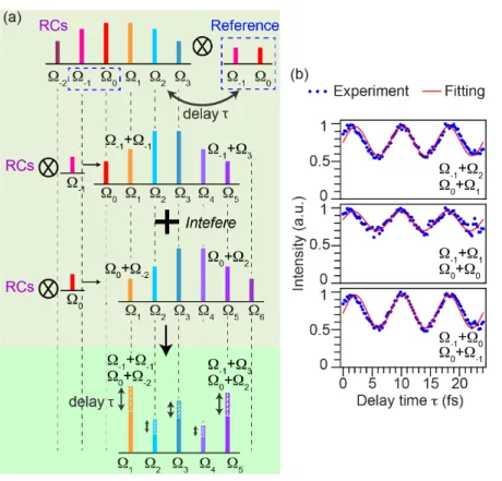
nonlin-ear optical crystal; SM, spectrometer.
Figure 2.3 shows details of interfering process. As a typical example, we hereby show the case where the spectrum has six components (refer to chap-ter 4). At the nonlinear optical crystal, the two arms mix with each other and produce two replicas of the original spectrum. As shown in figure 2.3(a), frequencies of two replicas are actually shifted by 2∆Ω (by taking a sum with Ω−1) and 3∆Ω (by taking a sum with Ω0). Then two replicas interfere with each
other, making overlapped frequencies serve as five SFG components (refer to 2.3(b)). Here, the five SFG components are phase correlated with the original spectrum.
2.3. PRINCIPLE OF SPIDER SYSTEM
Figure 2.3: Mechanism of retrieving phases of a spectrum with six compo-nents in SPIDER system. (a), The process of interfering. (b), Typical examples of intensity oscillations of interfered signals obtained by spectrometer. RCs, Raman components.
With delay time τ existing in the reference arm, electric-field intensities of SFG components are given as
ImSF G = |Em+1E−1R eiΩ−1τ + EmE0Re iΩ0τ|2 = |Em+1E−1R |2+ |EmE0R| 2 + 2|Em+1E−1R EmE0R|cos((ψm+1− ψm) + (ψ−1R − ψ0R) − ∆Ωτ ) (2.26)
where variables with superscript R represent the reference arm. Apparently, intensity oscillations of interfered SFG components are sinusoidal functions of delay time τ , and the period of each oscillation is fixed at 1/∆Ω = 8.02 fs.
2.3. PRINCIPLE OF SPIDER SYSTEM
of SFG components, with three different frequencies, Ω2, Ω3, and Ω4,
respec-tively. By fitting intensity oscillations with sine functions, we can retrieve spectral phases of SFG components. Certainly, here we need to take into ac-count precision of fitting, which affects reliability of phase measurement via SPIDER system. Refer to relevant discussions in chapter 5. Hereafter, accord-ing to interferaccord-ing process in equation 2.26, we are able to extract fundamental phases (i.e., phases of the original spectrum). Refer to [76] for more details.
Equiped with numerical exploration for phase manipulation and SPIDER system for phase measurement, we are able to thoroughly harness phases of a broad spectrum, and achieve ultrafast pulses near TL condition. After ma-nipulating amplitudes and phases of a spectrum, we can use the following equation to reconstruct normalized electric field intensity waveforms in the time domain. Ipulse = | m X k=−2 Ek∗ exp[i(2πΩkt + ψk)]|2/( m X k=−2 Ek)2 (2.27)
Bibliography of Chapter 2
[66] A. Yariv and P. Yeh. Photonics: optical electronics in modern
communi-cations. the sixth edition. Oxford Univ. Press, Oxford, 2006.
[67] K. Yoshii, J. K. Anthony, and M. Katsuragawa. “The simplest route to generating a train of attosecond pulses”. In: Light: Sci. & Appl. 2 (2013), e58.
[68] M. Katsuragawa and K. Yoshii. “Arbitrary manipulation of amplitude and phase of a set of highly discrete coherent spectra”. In: Phys. Rev. A 95 (2017), p. 033846.
[69] T. Jannson and J. Jannson. “Temporal self-imaging effect in single-mode fibers”. In: J. Opt. Soc. Am. 71 (1981), p. 1373.
[70] J. Azana and M. A. Muriel. “Temporal self-imaging effects: theory and application for multiplying pulse repetition rates”. In: IEEE J. on
Se-lected Topics in Quan. Elec.7 (2001), pp. 728–744.
[71] J. Fatome, S. Pitois, and G. Millot. “Influence of third-order dispersion on the temporal Talbot effect”. In: Opt. Comm. 234 (2004), pp. 29–34. [72] D. J. Kane and R. Trebino. “Characterization of arbitrary femtosecond
pulses using frequency-resolved optical gating”. In: IEEE J. Quantum
Electron29 (1993), p. 571.
[73] M. Schultze et al. “Delay in photoemission”. In: Science 328 (2010), pp. 1658– 1662.
[74] I. A. Walmsley and V. Wong. “Characterization of the electric field of ultrashort optical pulses”. In: J. Opt. Soc. Am. B 13 (1996), pp. 2453– 2463.
BIBLIOGRAPHY OF CHAPTER 2
[75] C. Iaconis and I. A. Walmsley. “Spectral phase interferometry for direct electric-field reconstruction of ultrashort optical pulses”. In: Opt. Lett. 23 (1998), pp. 792–794.
[76] T. Suzuki, N. Sawayama, and M. Katsuragawa. “Spectral phase mea-surements for broad Raman sidebands by using spectral interferome-try”. In: Opt. Lett. 33 (2008), pp. 2809–2811.
Chapter 3
Experimental system
Figure 3.1 shows the main experimental system, which consists of three parts: generation of a discrete broadband spectrum, amplitude and phase manipu-lations, and measurement of spectral phases. The three sections below corre-spond to details of each part.
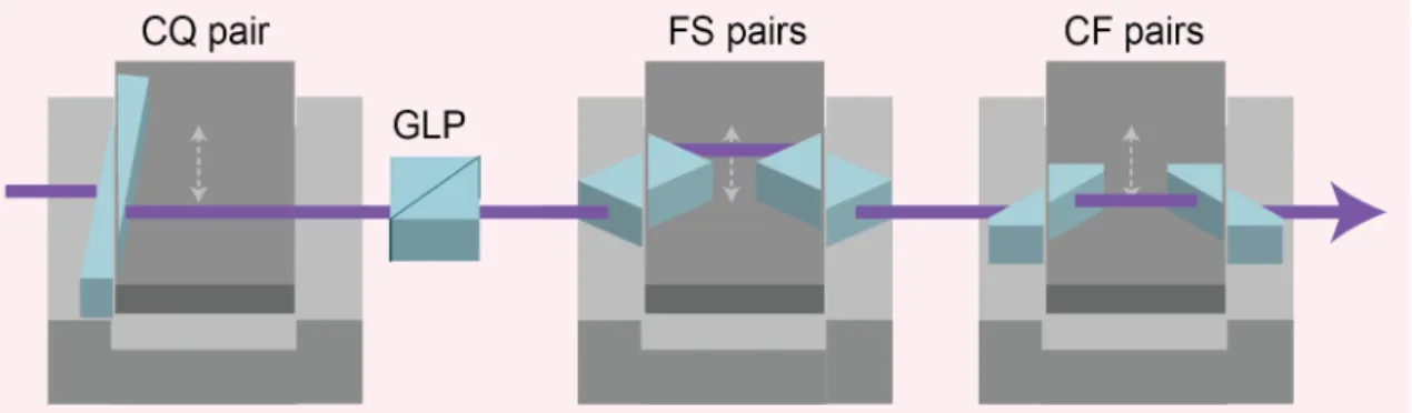
Figure 3.1: The main experimental system, consisting of three parts: gen-eration of a discrete broadband spectrum, amplitude and phase manipula-tions, and measurement of spectral phases. This diagram shows a top view of the system. P0–P3 represent different positions on optical axis. LN,
liq-uid nitrogen; para-H2, para-hydrogen; CQ, crystal quartz; GLP, calcite Glan
laser polarizer; FS, fused silica; CF, calcium fluoride; PaM, parabolic mirror; LPF, long-wavelength pass filter; BBO, β-barium-borate crystal (Type-1, 10 µm thick); SM, spectrometer.
3.1. RAMAN GENERATION
3.1
Raman generation
The interaction medium – gaseous para hydrogen–is filled into an enclosed 15 cm long copper chamber, with an adiabatic temperature of 77 K, supported by a liquid nitrogen cryostat. The purity of para hydrogen is up to 99.9%.
3.1. RAMAN GENERATION
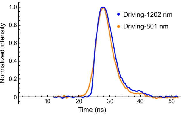
Figure 3.3: Pulse envelopes of two driving lasers. These pulse envelopes were obtained through a fast photon diode (Thorlabs DET025A), having a width of about 7 ns.
As figure 3.2 shows, two coaxial driving lasers—Ω−1, 1,201.6350 nm, 6.0 mJ
and Ω0, 801.0820 nm, 6.0 mJ—have an envelope duration of about 7 ns (at full
width at half maximum) and good Gaussian beam profiles. Overlapping at the chamber center of para hydrogen, the beam radii and peak intensities of Ω−1 and Ω0 are 150 µm, 120 MW/cm2 and 120 µm, 180 MW/cm2, respectively.
Two-photon detuning of vibrational Raman scattering is about δ = - 300 MHz. Refer to figure 3.3 for pulse envelopes of two driving lasers.
What to note here is that both the density of para hydrogen gas [77–79] and the lens pair of two driving lasers in front of cryostat have been carefully calibrated, for the sake of optimal Raman scattering [80]. Here, we merely use the optimal parameters: 8 × 1019 cm−3 for the density of para-hydrogen gas,
and focal lengths of 400 mm (with respect to Ω0) and 250 mm (with respect to
Ω−1) for the lens pair.
3.2. MANIPULATION DEVICES
components (see the insert at position P1), which has a constant frequency
spacing of about ∆Ω = Ω0-Ω−1 = 124.75 THz.
3.2
Manipulation devices
The middle part of figure 3.1 shows the devices of amplitude and phase ma-nipulations. See also figure 3.4 for an enlarged view. We use a pair of wedge-shaped crystal quartz (CQ, positive uniaxial) as waveplate. The optical axis of CQ is orientated 45 degrees to the direction of linear polarization of incident laser. The transmission direction of calcite Glan laser polarizer (GLP) is set parallel to the polarization direction of incident laser. Two pairs of triangular-pole-shaped fused silica [81], and also two pairs of trapezoidal-triangular-pole-shaped calcium fluoride [82] are used for controlling phases.
Figure 3.4: The devices of amplitude and phase manipulations. Gray dashed arrows depict translation directions of stages.
As shown in figure 3.4, all prism pairs are mounted on uniaxially movable stages (Sigma Tech FS-1020X, driven by a Sigma Tech FC-101 controller). This set of devices can translate over a range of about 20 mm, with high pre-cision and fine resolution (about 0.1 µm), and excellent reproducibility. For convenience, the whole set of devices are controlled by LabVIEW programs. In fact, according to our analyses and experiments, the resolutions needed for precise control are about 5 µm for MA, and 1 µm for MP, respectively; and the range needed for flexible control are about 10 mm for MA, and 2 mm for MP,
3.3. SPIDER SYSTEM
respectively.
Besides, as shown in figure 3.4, all prism pairs are slightly separated by a parallel distance of 10 µm using a tungsten wire. The parallel gap is per-pendicular to light propagation so that the stage can move along it to change thickness linearly.
Details of the scales of manipulation devices are shown in Appendix A.
Basically, we would like to perform experiments only by changing the thick-nesses of waveplate and dispersive plates, hence the prisms in pairs should not shift beam path considerably after transmitting. Besides, all prisms are placed carefully to make use of their Brewster angles, through which we ex-pect to reduce reflection loss at surfaces. Depending on sex-pectral mode, optical path slightly shifts in parallel in some section of prism pairs, but such a shift is really a small amount and does not affect the entire propagation.
3.3
SPIDER system
The rightmost part of figure 3.1 shows SPIDER system, which is slightly mod-ified for discrete spectra. See also figure 2.2 in chapter 2. Figure 2.2 shows a schematic diagram of SPIDER system.
Relying on frequency spacing of ∆Ω=124.75 THz, translation of the delay stage on reference arm needs to reach a resolution of about 10 nm over a range of several micrometers. The actual delay stage employed here (nPoint Inc., nPoint LC. 400) is capable of reaching a resolution of less than 1 nm over a range of more than 100 µm. Two arms of Raman components are sent through parallel paths to the parabolic mirror and con-focused onto the sur-face of a 10 µm thick BBO (β-barium-borate, Type-1, transmitting range of 3,500–190 nm) crystal. BBO crystal has a large nonlinear coefficient, and can be phase matched over a wide range of wavelengths. Hence it is eligible for sum frequency generation (SFG)–wavelengths from 601 to 267 nm–in our work.
3.3. SPIDER SYSTEM
we can translate the position and twist the angle of BBO crystal for optimal phase matching.
We use a spectrometer (Ocean Optics USB 4000 or Andor SOLIS MS-257, viable wavelength range: 1,100–200 nm) to monitor intensity oscillations of SFG components (refer to figure 2.3). The translation of delay stage and the record of intensity oscillations of SFG components via spectrometer in real time are controlled by LabVIEW programs.
Nevertheless, as we expect to perform experiments to verify numerical ex-ploration, we have to experimentally scan each point (i.e. a combination of two thicknesses) explored. This process actually yields a large quantity of raw data. Therefore, how we can translate the delay stage to scan intensity oscillations of SFG components quickly and efficiently becomes the key point whether or not this SPIDER system can be a substantial technique for retriev-ing phases.
Bibliography of Chapter 3
[77] J. P. Wittke and R. H. Dicke. “Redetermination of the hyperfine split-ting in the ground state of atomic hydrogen”. In: Phys. Rev. 103 (1956), pp. 620–631.
[78] W. K. Bischel and M. J. Dyer. “Temperature dependence of the Raman linewidth and line shift for the Q(1) and Q(0) transitions in normal and para-H2”. In: Phys. Rev. A 33 (1986), pp. 3113–3123.
[79] S. W. Huang, W. J. Chen, and A. H. Kung. “Vibrational molecular mod-ulation in hydrogen”. In: Phys. Rev. A 74 (2006), p. 063825.
[80] K. Morimune. “Efficient generation of high-order stimulated vibrational Raman scattering”. In: Master Thesis (2016).
[81] I. H. Malitson. “Interspecimen comparison of the refractive index of fused silica”. In: J. of the Opt. Soc. of Am. 55 (1965), pp. 1205–1209.
[82] M. Daimon and A. Masumura. “High-accuracy measurements of the re-fractive index and its temperature coefficient of calcium fluoride in a wide wavelength range from 138 to 2326 nm”. In: Appl. Opt. 41 (2002), pp. 5275–5281.
Chapter 4
Results
In this chapter, I will show main experimental results, which in fact encompass three sections: results of amplitude manipulation, results of phase manipula-tion, and ultrafast pulses achieved. Each section consists of different number of Raman components (five, six, and seven).
Naturally, we made experiments and acquired results in sequence. That is, we started to carry out experiments from manipulating amplitudes and phases, and producing ultrashort pulses of five Raman components (spanning 2,403 to 481 nm); then did the same on six RCs (spanning 2,403 to 400 nm); and ultimately on seven RCs (covering 2,403 to 343 nm). Therefore, I will introduce the results in turn, while declaring key points and operating procedures within five RCs.
However, in fact, all the techniques of manipulation and even reconstruction of ultrafast pulses are processed in the same way for different number of Ra-man components. The main difference among them is that with the number of Raman components increasing, the difficulty of arbitrarily manipulating both amplitudes and phases is elevated, in terms of numerical exploring range (for MA), and experimental resolution (for MP). Detailed discussions are provided in chapter 5.
To be specific, in section 4.1, I will show the photos of Raman scattering, which is our light source to be manipulated.
4.1. PHOTOS OF RAMAN COMPONENTS
In section 4.2, I will first show key points and practical procedures of manip-ulating amplitudes. Then I will show experimental results obtained, including actual intensity (in terms of power) and amplitude distributions achieved. As for detailed precision and error estimations, please refer to chapter 5.
In section 4.3, similarly, I will first show key points and difficulties of phase manipulation in experiment, which, comparing to MA, are more sophisticated; then list out practical procedures of MP for locking the target (i.e., near Fourier transform limited conditions); briefly show precision of phase retrieval process; and finally show the phase distribution after MP. Please also refer to chapter 5 for detailed discussions of precision in MP.
4.1
Photos of Raman components
Figure 4.1: Photos of Raman components (from 1,202 to 240 nm). The red dot of 2,403 nm was not observed, and was just exhibited as a mark to represent such Raman component. PBP, pellin broca prism, which spatially separates coaxial Raman components for photo shooting; dashed line indicates the Ra-man components to be Ra-manipulated in experiment.
Figure 4.1 shows photos of a series of high-order Raman components [83–87], by adiabatically driven vibrational transition of para hydrogen molecules (tem-perature: 77 K, and density: 8×1019 cm−3). These Raman components were
4.1. PHOTOS OF RAMAN COMPONENTS
(125 THz) to Ω7(1250 THz), with a frequency spacing of about 125 THz. Refer
to figure 4.2 for their pulse envelopes.
Figure 4.2: Pulse envelopes of generated Raman components. These pulse envelopes were obtained through a fast photon diode (Thorlabs DET025A). The black line shows the trigger pulse, which was scattered light of 801 nm far before para hydrogen cell
As shown in figure 4.1, the coaxial Raman components (RCs) were spatially separated by a pellin broca prism (PBP) and made incident on screens for shooting photos. All Raman components were shot one by one using a digital camera, and then trimmed by photo editor at same conditions and exhibited as in figure 4.1.
Note that in order to make beam profiles more viewable, we used different kinds of color filters when taking shots, thus recording different brightness regardless of their original intensities. We also used different kinds of screens to project each component: a normal white paper to project Raman components from 601 to 240 nm, and an infrared card to project components of 801 nm and 1,202 nm, which are in the infrared wavelength range. The component,
4.2. RESULTS OF AMPLITUDE MANIPULATION
2,403 nm, in mid-infrared wavelength range, was not directly observed, and we simply presented it as a round spot. Because we could not capture it through proper approaches in experiment.
What is notable here is that these beams were generated efficiently and coax-ially without any constraints of phase matching conditions (owing to the fea-ture of adiabatic driving vibrational Raman coherence); had excellent Gaus-sian beam profiles (refer to figure 4.1); and were discrete in the frequency domain with a frequency spacing of ∆Ω = 125 THz, which is essential and adequate for latter amplitude and phase manipulations.
Given the above brilliant light source–a highly discrete broadband spectrum with good Gaussian beam profiles, we could move on to manipulating its am-plitudes and phases.
4.2
Results of amplitude manipulation
This section shows results of amplitude manipulation on five, six, and seven Raman components, respectively. I will begin with five RCs. Meanwhile, I will show key points of implementing experiments, concrete procedures of manipu-lating amplitudes, and finally exhibit achieved amplitudes. Afterwards, I will show similar results of six and seven Raman components.
4.2.1
Results of amplitude manipulation of five Raman
components
Using the device of amplitude manipulation shown in figure 3.4, we carried out experiments to tailor all intensities (in terms of power).
4.2. RESULTS OF AMPLITUDE MANIPULATION
Figure 4.3: Results of amplitude manipulation of five Raman components. (a), Original powers of five Raman components. Ω−2, 8.0; Ω−1, 704.3; Ω0, 305.7; Ω1,
42.9; Ω2, 25.0 (kW), respectively. (b), MA process. Cyan numbers with arrows
in Ω−2indicate manipulating process: 1, initial scanning for determining basic
parameters of power oscillations; 2, fitting with sinusoidal functions accord-ing to initial scannaccord-ing; 3, experimental exploration of the optimum around the numerically expected optimal thickness. (c), Target (green) and achieved (red) power distributions. (Raman component: target (kW), achieved (kW)): (Ω−2:
3.3, 3.3), (Ω−1: 16.4, 14.7), (Ω0: 15.7, 12.9), (Ω1: 13.6, 13.7), (Ω2: 7.9, 7.4),
re-spectively; gray columns indicate achieved amplitude distribution normalized by the maximal intensity of Ω−1. Typical power fluctuations are in a range of
about ±3%– ± 7%, marked as error bars (standard deviations) above the red columns.
As shown in log10-scale in figure 4.3(a), the original powers of five Raman
components before manipulating were Ω−2, 8.0; Ω−1, 704.3; Ω0, 305.7; Ω1, 42.9;
Ω2, 25.0 (kW), respectively. These powers were measured directly by an energy
meter (Ophir NOVA 2), with an envelope duration of about 7 ns. Also refer to figure 4.1. The powers before MA are vastly different from each other, even
4.2. RESULTS OF AMPLITUDE MANIPULATION
with different levels–from the lowest 8 kW to the highest 704 kW. Given such preconditions, through MA process, we expect to achieve near flat intensities and thus near flat amplitudes, which contribute to reconstructing ultrafast pulses. As a result, we set near flat distribution of intensity (or amplitude) as our target.
To realize our target, basically, the adjustment would be the direction of decreasing powers, namely, maintaining the powers of Ω−2 and Ω2–which were
very low–to their maximal values, and meanwhile suppressing powers of the rest components.
What is worth noting is that although here we set near flat distribution of powers for producing ultrafast pulses, we are actually able to arbitrarily ma-nipulate these intensities, i.e., to produce some complex distributions. Nev-ertheless, when the complexity of target distribution increases, we have to extend the range of numerical exploration to approach such target. That is, the difficulty of MA escalates following the complexity of target distribution.
As an optical technology in practical use, the difficult point is that we can not directly and analytically calculate intensity oscillations and further pre-dict where to find the exact solution. Instead, we numerically explore an ap-proximate solution that approaches the target well with high precision. Below shows how we were able to realize such idea.
To numerically explore optimal solution for the intensity distribution of tar-get, we have to grasp concrete behaviors of power oscillations of all five (later six and seven) Raman components over a wide range. As discussed in chapter 2, the power of each Raman component oscillates periodically with respect to the thickness of waveplate (i.e., CQ pair).
In general, first we can sweep through a range of a few millimeters of wave-plate thickness (initial scanning). Next we can fit initial scanning with sinu-soidal functions, and obtain basic parameters of each oscillation–period and initial intensity. Then we can predict intensity oscillations of all RCs over a fairly wide range (far beyond the range of initial scanning). That is to say, we can numerically explore an optimal thickness to approach the target over a