CRR WORKING PAPER SERIES A
Center for Risk Research
Faculty of Economics
SHIGA UNIVERSITY
1-1-1 BANBA, HIKONE, SHIGA 522-8522, JAPAN Working Paper No. A-17
Labor Supply of Japanese Married Women: Sensitivity Analysis and a New Estimate
Shingo Takahashi, Masumi Kawade and Ryuta Ray Kato August 2009
Labor Supply of Japanese Married Women:
Sensitivity Analysis and a New Estimate
1Shingo Takahashi
2Masumi Kawade
3Ryuta Ray Kato
4August 2009
Abstract
We conduct a comprehensive analysis of the existing literature on the labor supply of Japanese married women using the Japanese Panel Survey of Consumers. We first conduct a detailed sensitivity analysis of the estimates of the wage elasticity to various economic and statistical assumptions used in the past studies. We then provide a new estimate of the labor supply model that simultaneously controls for wage endogeneity, sample selection into labor force as well as the possibly endogenous selection between different segments of the non-linear and often discontinuous budget constraint in a joint maximum likelihood estimation. We reject the assumption of wage exogeneity. The wife's labor market experience appears to be a valid excluded instrument, which validates most of the model specifications in the prior literature. The assumption of no-sample selection bias is rejected. Our new estimate shows that there are notable differences in the labor supply behavior of women who choose different segments of the budget constraint. In particular, the wage elasticity of women who work within the 1.03 million yen ceiling is twice more negative (-1.28) than that of women whose income exceeds the 1.41 million yen ceiling (-0.60). The wage elasticity smaller than -1 for the former type of women suggests that they may be adjusting their hours of work so as to contain their income within the 1.03 million yen ceiling.
Keywords: Female labor supply; Spousal deduction; Social Security System; Non-linear
budget constraint
JEL Classification: J20, H24
Correspondence: Ryuta Ray Kato, Visiting Research Fellow at Center for Risk
Research, Faculty of Economics, Shiga University (email: [email protected])
1 The Grants-in-Aid for Scientific Research of Scientific Research C (No. 19530294) by Japan
Society for the Promotion of Science (JSPS) is gratefully acknowledged. We also express our gratitude to the Institute for Research on Household Economics for their kind permission to use the Japanese Panel Survey of Consumers (JPSC) for our research.
2 Graduate School of International Management, International University of Japan (email:
3 Faculty of Economics, Niigata University (email: [email protected])
4 Graduate School of International Relations, International University of Japan
1.
Introduction
The elasticity of hours worked with respect to wage (wage elasticity) for Japanese married women is an important parameter on which various policy decisions can be made. In an aging Japan, a further decrease in labor force in the near future is forecasted to be
inavoidable1, and the government policy to stimulate female labor supply can be considered
as an effective policy to achieve stable economic growth in the future2. The effectiveness
of such a policy depends upon to what extent key determinants of female labor supply can precisely be estimated, and the precise estimation of the wage elasticity of Japanese married females is obviously one of the most important tasks.
However, there is a lack of studies that estimate wage elasticities. Moreover, the esti-mated wage elasticities vary considerably among the past studies, ranging from a negative estimate of -0.51 to a positive estimate of 0.26 (see Section 3). Disparate estimates of wage elasticities in the literature hinder the usefulness of such estimates in the policy analysis.
Disparate estimates could stem from different economic and statistical assumptions that underlie each study. In fact, in the past literature, there are significant differences in (1) the choice of explanatory variables, (2) the exogeneity assumption of wage and the choice of instruments, and (3) the assumption concerning whether selection into labor force is non-random. Since each of the past study does not provide a sensitivity analysis of its estimate to the above mentioned differences, it is not possible to tell whether disparate estimates stem from different economic and statistical assumptions, or merely from different data sources.
The purpose of this paper is two folds. First, we conduct a sensitivity analysis of the wage elasticity to various economic and statistical assumptions using a single data set.
1See National Institute of Population and Social Security Research (2008).
2We simulated the effect of an aging population in Japan on taxation, social security and economic growth, and also found that a drastic decrease in labor force would result in a decrease in economic growth in the future. See Kato (2002), and Ihori, Kato, Kawade, and Bessho (2006).
We use a sample from the Japanese Panel Survey of Consumers covering 1994-2003. We consciously vary assumptions one at a time to highlight the sensitivity of the estimate of wage elasticity to different assumptions. We pay particular attention to (i) the effect of the choice of explanatory variables on the estimates of wage elasticity, (ii) the validity of the exclusion restrictions in the 2SLS procedure, (iii) the sensitivity of the estimate of wage elasticity to the statistical control for the sample selection. To our knowledge, no other studies provide detailed sensitivity analysis of the wage elasticity of Japanese married women. Therefore, results presented in this paper should serve as an extremely useful resource for the study of female labor supply in Japan.
It is well known that the spousal deduction and the social security system in Japan causes a piecewise linear and often discontinuous budget constraint for the secondary income earner in a household. It is commonly believed that such a non-linear budget constraint causes married women to adjust their labor supply in order to stay in a particular segment of the budget constraint. Although past studies have estimated the female labor supply sepa-rately for the part-time workers and the full-time workers, these studies have not sufficiently investigated the difference in the labor supply behavior of women who choose different seg-ments of the budget constraint. Thus, the second purpose of this paper is to provide a new estimate of the female labor supply model that highlights the difference in the labor supply behavior of the women in different segments of the non-linear budget constraint. In particular, we estimate wage elasticity separately (but jointly) for different segments of the non-linear budget constraint. We simultaneously control for (1) a possibly endogenous selection into different segments of the budget constraint, (2) non-random selection into labor force, as well as (3) wage endogeneity.
We organize our paper as follows: Section 2 describes the tax and social security system in Japan. Section 3 discusses the prior literature. Section 4 presents the data and variables.
Section 5 conducts the sensitivity analysis, and Section 6 presents our new estimate of the female labor supply that simultaneously controls for wage endogeneity, sample selection bias as well as a possibly endogenous selection into different segments of the budget constraint. Section 7 concludes.
2.
Tax and social security system in Japan
Table 1 shows the 2002 income tax schedule for an employed worker. Employed workers are entitled to receive the employee tax deduction. Table 2 shows the employee tax deduction schedule. The amount of deduction depends on one’s income. Due to the tax deduction schedule, workers begin to pay tax only after their income exceeds 1.03 million yen. Besides the employee deduction, a married worker is entitled to receive a spousal tax deduction, depending on the spouse’s income level. In the following, we briefly explain the spousal tax deduction system in Japan. Throughout this section, we refer to the husband as the primary income earner, and the wife as the secondary income earner.
In 2002, the husband is given the annual tax deduction of 760 thousand yen when the wife’s annual income is less than 700 thousand yen. When the wife’s income exceeds this threshold, this spousal tax deduction is reduced by 50 thousand yen for each 50 thousand yen earned by the wife. When the husband’s income is less than 10,000 thousand yen, this reduction in the spousal deduction continues until the wife’s income reaches 1,410 thousand yen. When the husband’s income is greater than 10,000 thousand yen, this reduction continues until the wife’s income reaches 1,030 thousand yen, then it becomes zero once the wife’s income exceeds 1,030 thousand yen threshold.
Thus, the reduction in the spousal tax deduction is almost one-to-one. When husband’s income is less than 10,000 thousand yen, spousal deduction can be approximated by the
following
SpousalDeduction = 760 f or 0 ≤ Yw < 700 (1)
= 1, 410 − Yw f or 700 ≤ Yw ≤ 1, 410 (2)
= 0 f or Yw > 1, 410 (3)
where Yw is the wife’s annual income. All the figures above are in thousand yen. When the
husband’s income is greater than 10,000 thousand yen, we replace equation (2) by “=1,410
-Yw for 700 ≤Yw≤1030”, and replace equation (3) by “=0 for Yw>1030”. The spousal
deduction up to wife’s income equal to 1,030 thousand yen is based on the Allowance
for Spouses (AS) tax legislation. The spousal deduction for wife’s income between 1,030
thousand and 1,410 thousand yen is based on the Special Allowance for Spouses (SAS) tax legislation. In other words, only a household with husband’s income less than 10,000 thousand yen is eligible for SAS. In our sample, virtually all the working women are eligible for SAS (99.2% of the working women sample). Thus, the discussion that follows will mostly assume SAS eligibility.
This tax deduction system causes a highly non linear budget constraint for married women, majority of whom is the secondary earners. To see this more clearly, let w be the
wife’s hourly wage, h be the wife’s hours of work, tW be the wife’s income tax rate, tH be
the husband’s income tax rate, X be the husband’s annual income considered exogenous, and D be the tax deduction that the husband could claim other than the spousal deduction. The employee tax deduction has the form aY +b. Thus, the total household income can be written as Household Income = wh − [wh − (awh + b) | {z } Employee deduction ]tW + X − [X − D − (1410 − wh) | {z } Spousal deduction ]tH (4) = w[1 − (1 − a)tW − tH] | {z } W if e0s af ter−tax wage h + btW + 1410tH + X(1 − tH) + DtH | {z }
Intercept of the budget constraint
Thus, the effective marginal tax rate for the wife whose husband is eligible for SAS is
[1 − (1 − a)tW − tH] in the income range between 1,030 and 1,410 thousand yen. When the
wife’s income is less than 1,030 thousand, the marginal tax rate is equal to the husband’ tax rate since she does not have to pay her own income tax until her income reaches that threshold. Thus, wife’s effective marginal tax rate jumps at the threshold income of 1,030 thousand yen. When wife’s income exceeds 1,410 thousand yen, wife’s marginal tax rate is
equal to [1 − (1 − a)tW] only, since the spousal deduction is eliminated.
The social security system in Japan causes additional complication to the budget con-straint. There are three categories in the social security system. Category I covers self-employed and non-self-employed. Category II includes (i) the Employee’s Pension Plan (EPP) that covers private sector employees and (ii) the Mutual Aid Association (MAA) that covers the public sector employees. Category III covers dependent spouses of the workers covered by the Category II social security system. When the wife’s income is less than 1,300 thou-sand yen, the wife is entitled for Category III retirement plan with no payment. However, when the wife’s income exceeds 1,300 thousand yen, the wife is required to pay the MAA
premium of 11.3 thousand yen per month (this is the premium in 2002).3 This causes a
sudden drop in the budget constraint.
When the wife’s income is less than 1.03 million yen, the husband typically receives an allowance from his employer as a fringe benefit. This fringe benefit is completely elim-inated when the wife’s income exceeds 1.03 million yen (see Abe 2009 for a more detailed discussion). Thus, this fringe benefit causes a further discontinuity in the wife’s budget constraint.
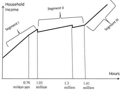
Considering above mentioned spousal deduction, the social security system and the fringe benefit, a budget constraint for the wife who is eligible for SAS can be described as
3The wife could choose EPP coverage instead. In this case the wife pays 8.65% of her annual salary as the EPP premium (this is the premium in 2002).
in Figure 1. We can roughly divide the budget constraint into 3 segments. Segment I is income between 0 and 1.03 million yen where she faces at most her husband marginal tax, and not her marginal tax and her husband’s marginal tax combined. There is a dip in the budget constraint at wife’s income equal to 1.03 million yen since the fringe benefit that the husband receives from his employer is cut off at this point. The 1.03 million yen threshold is often called ‘1.03 million yen ceiling’, since many married women attempt to contain their income below this ceiling. Segment II is the income range between 1.03 million and 1.41 million yen where she faces a combined marginal tax of her husband’s and her own. She also faces a dip in the budget constraint at income equal to 1.30 million yen due to the social security payment. Segment III is the income range above 1.41 million yen. At 1.41 million yen, the budget constraint could still be ‘dipped’. The budget constraint ‘recovers’
around the income equal to 1.44 million yen.4 In this sense, one may consider it better
to choose the budget segment starting from income equal to 1.44 million yen. However, the choice of this threshold is not particularly important since, theoretically, nobody would choose to work where the budget constraint is dipped. This segmentation is similar to Akabayashi (2006). Akabayashi replaced a dip in the budget constraint with a horizontal line in his structural estimation. The threshold of 1.41 million yen where spousal deduction is eliminated is often called ‘1.41 million yen ceiling’.
In order to fully take into account such a non-linear budget constraint, one needs to compute the likelihood that an individual chooses a particular budget segment given a pre-specified utility function. Then, one could estimate the labor supply parameters structurally by using maximum likelihood. Akabayashi (2006) estimates such a structural model. Although we do not attempt to incorporate the non-linearities in this sense, it is important to take into account the possibly different labor supply behaviors of wives
4Since she will start paying 11.3 thousand yen per month as social security payment, her annual income will not ‘recover’ until she earns more than 1,300+11.3×12≈1,435.6 thousand yen.
who choose different budget segments. One way to do so is to separately (but possibly jointly) estimate a labor supply equation for each segment. By doing so, we are assuming that wives in each segment have distinctly different behavior. This is not an unreasonable assumption. For example, it is widely believed that wives who choose Segment I have ‘income adjustment behavior’. More specifically, these wives are believed to adjust their hours of work so that their annual income is always below the 1.03 million yen ceiling. In an extreme case, the wife would supply labor so that her annual income is always constant, that is wh=constant, for which case the wage elasticity is always -1. The work disincentive effect of the 1.03 million yen ceiling has been the focus of the study of female labor supply in Japan (Oishi, 2003; Abe and Otake, 1995; Akabayashi 2006). Segment II is peculiar since it faces higher marginal tax rate plus the dips in the budget constraint. It turns out that there are only a few observations in our data set who have chosen this segment. In Segment III, there are no incentive for ‘income adjustment’.
In the past studies, labor supply is often estimated separately for part-time workers and full-time workers. None of the past studies estimated labor supply separately for dif-ferent budget segments. Thus, we are able to contribute to the literature by highlighting the differences in the labor supply behavior of women who choose different segments of the budget constraint. By separating samples into three segments, there is an additional prob-lem of the sample selection into different segments of the budget constraint. In Section 6, we estimate a model that simultaneously controls for possibly endogenous sample selection into different budget segments, in addition to the sample selection into labor force.
3.
Prior literature
Table 3 is a summary of 5 representative studies that report wage elasticities of Japanese women using a micro data (Oishi, 2003; Abe and Otake, 1995; Kuroda and Yamamoto,
2008a; Hill, 1989; Akabayashi, 2006). There are significant differences in the econometric method they utilized, the choice of explanatory variables as well as the choice of excluded instrumental variables. The estimated wage elasticity also vary among studies, ranging between -0.51 to 0.26.
Oishi (2008) uses a sample of 423 married women from Kokumin Seikatsu Kiso Chousa. Her model is a simple OLS. In addition to the usual explanatory variables such as non-wife income and the number of children, her labor supply equation contains household characteristics as well as asset variables. She finds negative and statistically significant wage elasticity of (-0.36). Since she uses OLS, it is implicitly assumed that wage is exogenous and that selection into labor force is random with respect to the error term in the hours worked equation.
Abe and Otake (1995) uses a large sample of married women from the General Survey
of Part-Time Workers (GSPT). Their model is a conventional one except that the labor
supply equation does not contain non-wife income. This is because their data contain no such variable. Their hourly wage is constructed by dividing the annual income by the annual hours worked. As Borjas (1980) notes, this could cause a downward bias in wage elasticity due to the division bias. To eliminate this bias, they use the reported hourly wage as the only instrument to estimate the model in a 2SLS procedure. Their estimates range between -0.51 and -0.24.
As noted in the previous section, spousal tax deduction causes a highly non-linear budget constraint. Akabayashi (2006) takes into account the non-linearity by structurally estimating a model, a model similar to Hausman (1980) and Moffit (1986). In order to reduce the computational burden, he includes only wage, non-wife income and wife’s age as explanatory variables. He finds positive and statistically significant uncompensated wage elasticity ranging between 0.10 and 0.24. Positive wage elasticity is consistent with the
majority of studies in the US. The data does not contain non-workers. Thus, the usual sample selection bias correction is not possible. The author uses truncated normal maximum likelihood to correct for the sample selection bias.
Kuroda and Yamamoto (2008a) estimate the inter-temporal substitution elasticity us-ing a sample from the Japanese Panel Survey of Consumers, the same data source we utilize in this study. They first estimate a wage offer equation. The predicted wage is then included in the hours worked equation to estimate the wage elasticity. The hours worked equation also includes the Heckman sample selection correction terms. Identification of wage effect is achieved by imposing exclusion restrictions. Their excluded instruments are labor market experience, industry dummies, the number of employees and prefectural average income. The wage elasticity is interpreted as the inter-temporal substitution elasticity due to the inclusion of the wife’s education, the husband’s education, year dummies and prefectural dummies in the hours worked equation, which are assumed to determine the marginal util-ity of wealth. They find that the inter-temporal wage elasticutil-ity is positive but small and
insignificant ranging between 0.05 and 0.20.5 The inter-temporal wage elasticity defines
the theoretical upper bound of the uncompensated wage elasticity (see MaCurdy 1981). MaCurdy finds that the inter-temporal substitution elasticity is very close to the uncom-pensated wage elasticity for the male sample. If this holds true for Japanese females, then the uncompensated wage elasticity could be positive, which confirms Akabayashi (2006). However, their estimate could have been driven by incorrect exclusion restrictions. They provide neither the test for over-identifying restrictions nor a qualitative justification for their choice of exclusion restrictions. Mroz (1987) in a detailed sensitivity analysis of the wage elasticity of married women in the US, shows that the wife’s labor market experi-ence is an invalid instrument. Intuitively, wife’s experiexperi-ence could be correlated with the
5Kuroda and Yamamoto (2008b) conduct a similar analysis using data aggregated by prefecture, age group and gender. They find positive wage elasticities ranging between 0.10 and 0.97.
wife’s unobserved taste for work. Thus, the use of possibly invalid instruments such as the experience could have caused a positive wage elasticity.
Hill (1989) uses the 1975 survey of women in Tokyo Metropolitan Area6 to estimate a
labor supply model for married women. She estimates labor supply separately for employees, and family workers (workers in informal sector) while controlling for trichotomous selection between non-working, working as an employee, and working as a family worker. Wage endogeneity is controlled for in the three stage least square procedure with wife’s labor market experience as the only excluded instrument. She finds that uncompensated wage elasticity is 0.26 for employees while it is 0.25 for family workers. Similar to Kuroda and Yamamoto (2008), she does not discuss the validity of the choice of instruments.
Thus, economic and statistical assumptions underlying each study vary considerably. First, the choice of explanatory variables differs considerably among these studies. Second, Oishi (2003) and Akabayashi (2006) treat wage as exogenous while Abe and Otake (1995), Kuroda and Yamamoto (2008a) and Hill (1989) treat it as endogenous. Third, sample selection into labor force is controlled for only in Kuroda and Yamamoto (2008a) and Hill (1989). Such differences raise several questions: Are the estimates of wage elasticity sensitive to a particular choice of explanatory variables? Are the estimates sensitive the the assumption of exogenous wage? Are the estimates sensitive to the assumption of non-random selection into labor force? How one might take into account all the sources of biases simultaneously? These are the questions that we answer in this paper.
4.
Data, variables, and summary statistics
Our sample is from the the Japanese Panel Survey of Consumers (JPSC) for the period between 1994 and 2003. This is a panel of randomly chosen 1500 Japanese women who were between age 23 and 34 at the initial survey which was in 1993, and an added panel of 500
women aged 24 to 27 in 1997. Most of the past studies used data sets that contain only part-time workers, omitting full-part-time workers and non-workers (GSPW for example). In contrast, JPSC contains full-time workers, part-time workers as well as non-workers, allowing us to control for sample selection biases as well as to include full-time workers. Furthermore, JPSC contains a rich set of personal and job characteristics. The disadvantage of JPSC is its small cross sectional units. The General Survey of Part-Time Workers contains 13,000 workers (1995 Survey).
The hourly wage variable is constructed as follows. Respondents report whether they are paid hourly, daily, weekly or monthly. When respondents are paid hourly, we use their reported hourly wage as the wage variable. When respondents are paid daily, we use (Reported Daily Wage)/8 as the wage variable, assuming that they work 8 hours per day. Annual hours workers is then computed as (Annual Pre-tax Income)/(Hourly Wage). This construction of the wage variable and the hours worked variable would minimize the division bias. This is because it would be easier for workers to recall their hourly wages and annual income than to recall their hours of work. Thus hourly wage and annual income would be more accurately measured, minimizing potential division bias. The construction of wage and annual hours worked variables is similar to Akabayashi (2006).
For women who are paid weekly or monthly, they report the monthly equivalent amount of salary. Unlike jobs that pay hourly or daily, jobs that pay weekly or monthly would also entail bonuses. This needs to be incorporated in the computation of hourly wage. Thus, we compute the hourly wage as (Annual Pre-tax Income)÷(Annual Hours Worked). Annual pre-tax income is reported by each respondent. Annual hours worked is constructed as (Annual Days Worked)×(Weekly Hours Worked)/5. Both annual days worked and weekly hours worked are reported in ranges in JPSC. We chose the middle point of each range for computation.
After-tax wage is computed based on the income tax schedule in Table 1, the employee deduction schedules in Table 2 as well as the spousal deduction schedule described in Section 2. The non-wife income is constructed as follows. First, from wife’s and husband’s annual income, we compute the intercept term of the budget constraint given in equation (5). This intercept can be interpreted as the wife’s virtual income. We then add income earned from assets by the wife and the husband to this virtual income. Finally, we subtract the amounts of social security payment made by the husband and the wife to construct the non-wife income. The amount of social security payments are estimated by assuming that the wife is covered by the MAA when her income exceeds 1.30 million yen, and that the husband is
covered by EPP7.
Our construction of non-wife income takes into account the income tax, but ignores other taxes such as the tax on the interest income. We could alternatively use the reported amount of tax and social security payment to construct the non-wife income. However, this variable is missing for a significant portion of the sample. Thus, in order to increase the sample size, we constructed the non-wife income in the way described in the previous paragraphs. In addition, the above construction of the non-wife income assumes that the
husband is an employee, and not a self-employed worker.8 Therefore, we restricted our
sample to the households where the husband is an employee.
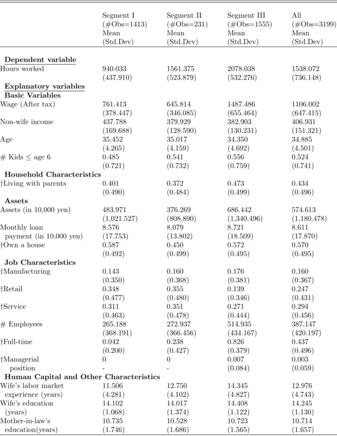
Table 4 shows the summary statistics of the variables utilized in this study separately for workers in the three budget segments described in Figure 1. There are 1413 person-year observations in the budget segment I, only 231 person-year observations in the segment II, and 1555 person-year observations in the segment III. The average hours worked is 940 hours for the segment I, 1561 hours for the segment II and 2078 hours for segment III.
7In 2002, the payment for MAA is 13.3 thousand yen per month while the payment for EPP is 8.65% of the salary.
8We assume that the wives pay the social security payment only after her income exceeds 1.30 million yen. This is not the case when the husband is a self-employed worker. When the husband is a self-employed worker, the wife pays the social security premium regardless of her income level.
Thus, hours worked is increasing with the budget segment. Average after-tax hourly wage is 761 yen for the segment I, 645 yen for the segment II and 1487 yen for the segment III. A drop in the wage in the budget segment II is due to the higher marginal tax rate for this budget segment. In fact, pre-tax wage rate is increasing with the budget segment (869 yen, 906 yen and 1721 yen for the budget segment I, II and III respectively). Average age is 35.4 for the segment I, 35.0 for the segment II and 34.2 for the segment III. Thus, women in the budget segment III are slightly younger than women in other segments, though the difference appears to be minor. Labor market experience is higher for the budget segment III (14.3 years) than for the segments II and III (12.7 years and 11.5 years respectively).
As is shown in Table 4, we utilize a number of explanatory/instrumental variables in the analysis. Wife’s age and the number of children below 6 are included virtually in any estimation of female labor supply. We include a dummy variable indicating if the wife is living with parents (her own parents and/or her husband’s parents). Wives living with parents are expected to work longer hours since parents typically provide household work, thus reducing wives’ housework. Several past studies include asset variables. (Assets) is the summation of household saving plus the value of securities. We also include the amount
of loan the family paid back during the month preceding the interview.9 In addition, we
include a dummy indicating if the household owns a house instead of living in a rented house.
We include three industry dummies (manufacturing, retail and services) to control for the possibility that industry characteristics could affect the hours worked. About 70% of all the working sample is in these three industries. We include three variables for job characteristics: full-time dummy, number of employees and a dummy variable indicating if the individual holds a managerial position. Job contents may be more intensive in a larger
firm, for full-time workers, and for managerial positions. Thus, we expect these variable to have a direct and positive impact on hours worked. Finally, we consider two human capital variables: wife’s education in years and her labor market experience in years. Kuroda and Yamamoto (2008a) used labor market experience as an excluded instrument. Our intention is to test whether or not these human capital variables are valid excluded instruments.
Figure 2-A shows the wife’s pre-tax annual income. Observations are heavily concen-trated in the income range between 0.9 million yen and 1 million yen, indicating that women are adjusting their hours of work so that their annual income is less than the 1.03 million yen ceiling. Figure 2-B shows the histogram of the wife’s after-tax wage rate. The wage rate is highly skewed to the right.
It is well known that the age-labor force participation profile for Japanese women is M-shaped. Nakamura and Ueda (1999) show that the labor force participation profile has its first peak at age between 20-24 (above 70%), drops to near 50% at age between 30-34, then attains its second peak (70%) at age between 45-49. In order to see if age-hours worked profile has a similar shape, Figure 2-C shows the average hours worked by age. The hours worked are the highest at age 24, exhibit some declining trend until age 40, then show a very slight increase afterwards. This trend could suggest that the age-hours worked profile is M-shaped, where the graph is capturing the dipping part of the profile. However, the change in hours worked after age 25 appears to be rather gradual. Thus, it is not conclusive whether or not the hours profile has an M-shape.
5.
Sensitivity analysis
In this section, we conduct a sensitivity analysis of wage elasticity to (1) the choice of explanatory variables, (2) the assumption of wage exogeneity and the choice of instruments, and (3) the statistical control for sample selection into labor force. We separately estimate
labor supply equations for the different segments of the budget constraint described in Figure 1. Since there are only 231 observations in Segment II, we decided that we are not able to obtain meaningful estimations for this budget segment. Thus, we dropped this budget segment from our analysis. By doing so, we implicitly assume that wives’ choice among budget segments is typically dichotomous, between segment I and segment III only.
5.1
Sensitivity to the choice of explanatory variables in OLS
First, we present the results for the budget segment III. Table 5 shows the results. OLS1 includes only the basic variables: wage, non-wife income, the wife’s age and the number of children below age 6. Wage elasticity is -0.34 and it is significant at the 1% level. Non-wife income has an unexpected positive sign. This could arise from the possible endogeneity of the non-wife income. If a wife with a high taste for work marries a husband with high income, the effect of non-wife income will be biased upward. A positive coefficient for the non-wife income is also found in Hill (1989).
Often, non-wife income is not included in the past literature. Does this affect the results? OLS2 excludes non-wife income from the model. The wage coefficient only slightly changes from -0.34 to -0.30. Past literature differs in the inclusion/exclusion of household characteristics such as the dummy for living with parents, and the asset variables. Oishi (2003) and Abe and Otake (1995) include these variables while Kuroda and Yamamoto (2008a), Akabayashi (2006) and Hill (1989) do not. OLS3 include these variables. Living with parents would increase hours of work by 3%. (Assets) has a positive effect on hours worked, which is consistent with the results reported by Kuroda and Yamamoto (See Table 3 of their study). The inclusion of these variables, however, has little impact on the estimated wage coefficient (-0.34).
OLS4 includes industry dummies. Only Abe and Otake (1995) include industry dum-mies. Though all the estimated coefficient for the industry dummies are statistically
sig-nificant, the estimated wage elasticity only slightly decreases from the OLS3 result of -0.34 to -0.365. In OLS5 we include the other job characteristics (the number of employees, the fulltime dummy and the managerial position dummy). The estimated wage elasticity ap-preciably changes to -0.481. This is a suggestive result. First, the number of employees and the full-time dummy have a positive effect on the hours worked, indicating that the job contents have a direct impact on hours worked. For example, job contents may be more demanding for larger firms and for a full-time position, thus requiring more hours of work. Without controlling for job characteristics, wage would pick up the positive effect of job contents on the hours worked, giving rise to an upward bias in the estimate of the wage elasticity. Since Oishi (2003), Kuroda and Yamamoto (2008a) and Akabayashi (2006) do not incorporate any job characteristics, their estimates could have been biased upward.
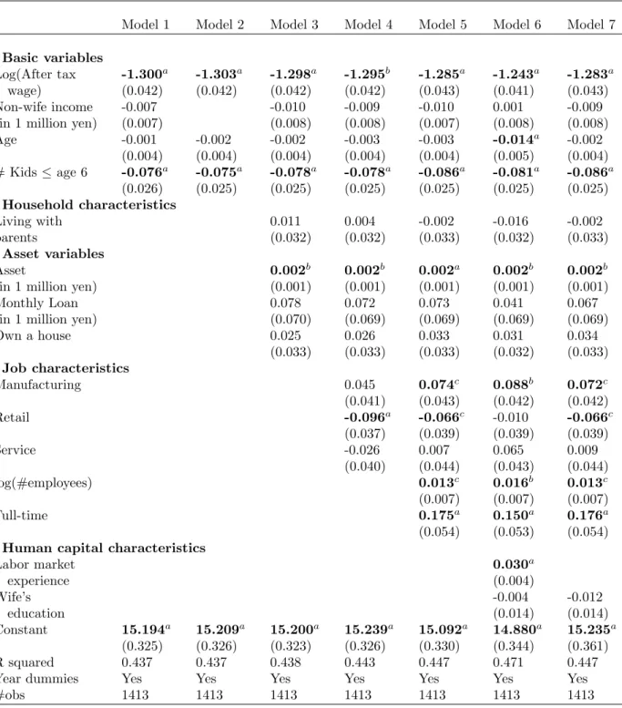
Finally, OLS6 includes the wife’s human capital characteristics (the wife’s labor market experience and the wife’s years of education). The wage coefficient decreases slightly from -0.48 to -0.50. In the past literature, the wife’s labor market experience is often used as an excluded instrument to control for wage endogeneity. In section 5.2, we will investigate if these human capital variables could be used as excluded instruments in the 2SLS procedure. Now, we replicate the same analysis for the budget segment I. Table 6 shows the results. In OLS1 to OLS4, the estimated wage elasticity stays at -1.30. The inclusion of job characteristics (the number of employees and the full-time dummy) in OLS5 does not change the wage coefficient appreciably (-1.29). The insensitivity of the wage elasticity to the inclusion of the job characteristic variables would mean that job characteristics are relatively homogeneous across different employers in the budget segment I. This is a reasonable result since most of the women in this budget segment are part-time workers, thus their tasks may be homogenous regardless of the employers (such as clerical work). The inclusion of human capital variables in OLS6 decreases the wage elasticity slightly to
-1.24. For all the models, we cannot reject the null hypothesis that wage elasticity for the budget segment I is smaller than -1. This implies a possible income adjustment behavior of these women.
5.2
Testing the wage exogeneity and the choice of instruments in
2SLS
The choice of instruments is a practical concern. A different choice of instruments could lead to significantly different estimates. Abe and Otake (1995) use the reported hourly wage as an excluded instrument to control for the division bias. Kuroda and Yamamoto (2008a) use labor market experience, average prefectural income, industry dummies and the number of employees as excluded instruments. Hill (1987) uses the wife’s labor market experience as the sole excluded instrument. None of these studies test the validity of their choice of instruments. This raises two questions: (i) are these instruments valid? and (ii) how sensitive is the estimated wage elasticity to the choice of instruments?
To answer to the first question, we use the test of orthogonality for a subset of instru-ments (Hayashi 2000:220). Consider the following model.
log(hour)it = β1log(wage)it+ βZ1it0 + ²it (6)
log(wage)it = αZ1it0 + γZ2it0 + uit (7)
where Z2it is the excluded instruments. Consistency of 2SLS requires that the set of
in-struments {Z0
1it, Z2it0 } be orthogonal to ²it. Equivalently, consistency requires that there is
no correlation between ²it and uit. Suppose that we add an additional vector of excluded
instruments Z3it. If we are confident that {Z1it0 , Z2it0 } satisfy the orthogonality conditions,
we can test wether the additional instruments Z3it satisfy the orthogonality conditions by
compute
C ≡ J − J1 →dχQ (8)
where J is the Hansen’s J statistics computed using {Z0
1it, Z2it0 , Z3it0 } as instruments. J1 is
the Hansen’s J statistics when using only {Z0
1it, Z2it0 } as instruments. Q is the number of
added instruments. If the resulting C statistic is too large, we reject the null hypothesis
that the additional instrument set Z3it is orthogonal to ²it. For this case, we reject the
model with added instruments in favor of the restricted model.
Conventional choice of instruments are wife’s background variables, such as her mother’s education and father’s education. Since the wife’s own human capital characteristics such as the labor market experience and her education are correlated with her wage, one may be tempted to use these variables as excluded instruments. In fact, Kuroda and Yamamoto (2008ab) and Hill (1987) use labor market experience as one of their excluded instruments. However, it is not a priori clear whether these variables would satisfy the orthogonality conditions. Mroz (1987) shows that the wife’s labor market experience is an invalid instru-ment. Intuitively, this is because the wife’s labor market experience is correlated with the unobserved taste for work. Thus, we first test whether the wife’ labor market experience and education can be used as excluded instruments.
Table 7 shows the results. This table shows several test statistics. The instrument relevance test is the F-test for the null hypothesis that excluded instruments are not jointly significant determinants of the wife’s wage. Hansen’s J is the test for the null hypothesis that the over-identifying restrictions are valid. C-test is already described above. The last column shows the test statistic for the null hypothesis that the log of wage is exogenous.
Let us first present the results for the budget segment III. The first row is our basic OLS model (OLS5 in Table 5). OLS wage elasticity is -0.48. The model IV1 uses only the mother’s education, its squared term, mother-in-law’s education and its squared term as the
excluded instruments. We refer to these excluded instruments as the ‘basic instruments’. We do not use father’s education since it has no explanatory power on the wife’s wage. Hansen’s J statistic does not reject the validity of the over-identifying restrictions (p-value=0.94). The wage exogeneity is rejected. The estimated wage elasticity is positive but statistically insignificant (0.079).
IV2 uses the wife’s labor market experience as an additional excluded instrument. The excluded variables are jointly significant. The C-test does not reject the orthogonality of the experience. Thus, the experience appears to be a valid excluded instrument. This result conflicts with Mroz’s (1987) finding that wife’e labor market experience is an invalid excluded instrument. In Japan, women have often been placed on a non-career track job with limited promotion prospects, which would reduce the incentive for women to stay
in the labor market to build a career.10 This could mean that the length of experience
is more likely to be determined by idiosyncratic circumstances, such as the availability of jobs nearby their houses or their financial needs rather than the wife’s unobserved taste for work. This could be a possible reason for the validity of the experience as an instrument. Wage exogeneity is rejected. The estimated wage elasticity slightly decreases to 0.067, and remains statistically insignificant.
IV3 adds the wife’s years of education as an additional excluded instrument. The p-value for the C-test is relatively low (0.068). Thus, the orthogonality of the wife’s education is rejected at the 10% level. Although not reported in the table, when we include wife’s education squared, the orthogonality of the wife’s education variables are rejected even at the 5% level. Thus, we consider that this model is misspecified. The estimated wage coefficient is significantly higher than the previous model (0.19) though it is not statistically
10Many Japanese firms provide a double track career system where a worker has a choice between the career-track job with the possibility of transfer within the company, and the non-career track job with no requirement to move. Though a worker has the choice, Debroux (2003;194) shows that women represent less than 4% of the career track positions in 2002.
significant.
The rejection of the orthogonality of the wife’s education may suggest that it should be included directly in the hours worked equation. To see if the experience can be excluded from the hours worked equation even when the wife’s education is included in the hours worked equation, we follow the same procedure. First, we estimate IV4 which includes wife’s education in the hours worked equation. We only use the basic instruments as the exclusion restrictions. Hansen’s J does not reject the validity of the over-identifying restrictions (p-value=0.90). Exogeneity of wage is rejected. The wage coefficient drops substantially to 0.009.
Now, we use the experience as an additional excluded instrument in IV5. The orthogo-nality of the experience is not rejected. Again, the experience appears to be a valid excluded instrument. Thus, our results provide statistical evidence that validates the frequent use of the wife’s labor market experience as an excluded instrument in the past studies. Wage exogeneity is strongly rejected. The wage coefficient increase to 0.096, though it is not statistically significant.
Finally, we test if job characteristics (industry dummies, the number of employees, full-time dummy and the managerial position dummy) can be used as excluded instruments. We take out these variables from the hours worked equation, then use them as additional excluded instruments. This model specification is similar to that of Kuroda and Yamamoto (2008a). IV6 shows the results. The C-statistic does not reject the orthogonality of the job characteristic variables, showing that Kuroda and Yamamoto’s (2008a) model specification is valid. The estimated wage elasticity is 0.07, though it is significant only at the 10% level. This estimate falls in the range estimated by Kuroda and Yamamoto (0.05 to 0.20). It should be noted that the p-value at which we fail to reject the orthogonality of the job characteristic variables is somehow small (p-value=0.18). Moreover, it will be shown that
the orthogonality of job characteristics is rejected for the budget segment I. Therefore, the appearance of the job characteristics as valid excluded instruments for the segment III could be due to the randomness in the data. For this reason, we consider the previous model (IV5) to be the most preferred model.
Thus, for the segment III, the 2SLS wage coefficient is much larger relative to the OLS results. The 2SLS wage coefficients mostly fall in a relatively narrow range [0.067, 0.096]. The wage coefficient is biased upward (0.19) when the wife’s education is mistakenly used as an excluded instrument.
Now we replicate the same analysis for the budget segment I. The bottom half of Table 7 shows the results. The OLS wage elasticity is -1.285. IV1 uses only the basic instruments as the exclusion restrictions. The excluded instruments are not significant determinants of the wife’s wage in the first stage regression. Nonetheless, the Hansen’s J does not reject the over-identifying restrictions.
IV2 includes the wife’s labor market experience as an additional excluded instrument. Now, the excluded instruments are significant determinants of the wage. The C-test does not reject the orthogonality of the experience. Thus, the wife’s labor market experience again appears to be a valid excluded instrument. The wage coefficient significantly drops to -3.94. IV3 includes the wife’s education as an additional excluded instrument. Similar to the case for the budget segment III, the orthogonality of the wife’s education is rejected at the 10% level. This rejection again indicates that the wife’s education should be included directly in the hours worked equation. IV4 includes the wife’s education directly in the hours worked equation, then uses the basic instruments as the only exclusion restrictions. The excluded instruments are not significant determinants of the wife’s wage, though Hansen’s J does not reject the validity of the over-identifying restrictions.
keeping the wife’s education in the hours worked equation. The excluded variables are now significant determinants of the wage. The C-test does not reject the orthogonality of the experience. Thus, the experience appears to be a valid excluded instrument. The exogeneity of wage is rejected. The estimated wage elasticity drops significantly from the OLS estimate of -1.28 to -4.01.
Finally, we test if the job characteristics can be used as excluded instruments for this budget segment. IV6 takes out the job characteristic variables from the hours worked equa-tion, then uses them as additional excluded instruments. In contract to the results for the budget segment III, the C-test strongly rejects the orthogonality of the job characteristics. This rejection shows that Kuroda and Yamamoto’s (2008a) model specification is not valid for this budget segment. Intuitively speaking, job characteristic variables are correlated with the unobserved job contents that directly affect the hours of work. Thus, IV5 appears to be the most preferred model.
For the segment I, the 2SLS wage coefficient decreases relative to the OLS results. The 2SLS coefficient falls in the range [-5.3, -4.0]. When invalid exclusion restrictions are imposed (the wife’s education and job characteristics), the wage coefficient tends to bias upward.
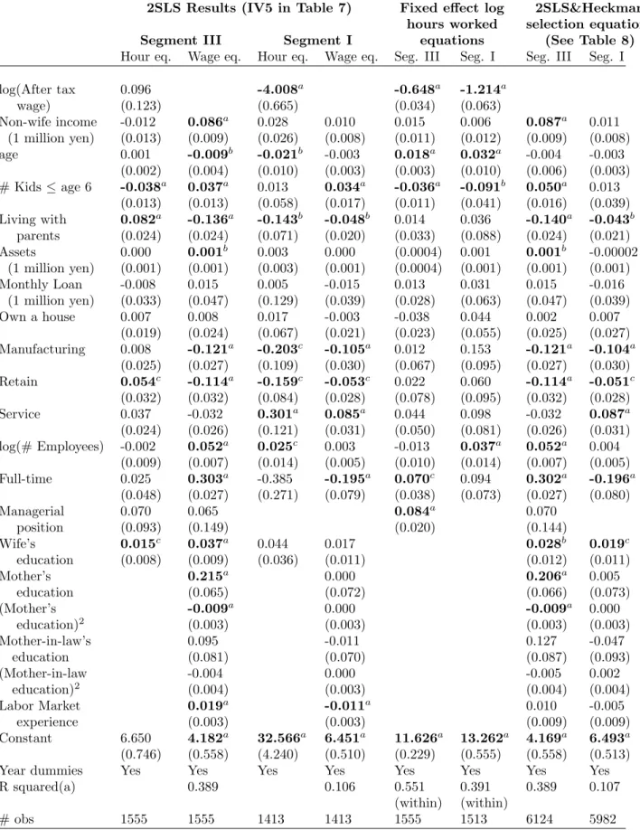
Table 10 shows the entire results for our preferred 2SLS models (IV5 for both budget segments). For the budget segment III, all the excluded instruments (except mother-in-law’s education) have statistically significant coefficients in the first stage regression. For budget segment I, among the excluded instruments, only the wife’s labor market experience has a significant coefficient in the first stage regression. The insignificant wage coefficient for the segment III and the weak instruments (especially for the segment I) indicate that we would need a more efficient method for addressing the wage endogeneity. In Section 6, we efficiently controls for wage endogeneity in a maximum likelihood framework.
5.2.1 Fixed effect estimation
Another way to control for wage endogeneity is to apply a fixed effect model. Table 10 shows the results. For the budget segment III, the wage elasticity drops substantially from the OLS result of -0.49 to -0.65. Intuitively, the fixed effect model eliminates the unobserved time-invariant effects, such as taste for work, that affect both wage and the hours worked in the same direction, thus eliminating an upward bias in the wage elasticity. For the segment I, the wage elasticity changes slightly (but not appreciably) from the OLS estimate of -1.28 to -1.24.
5.3
Selection bias
If sample selection into labor force is not random, the OLS estimate of the wage elasticity using only the sample of working women will be biased. Consider the following model:
log(hour)it = β1log(wage)it+ βZ1it0 + µit (9)
Iit∗ = Xit0γ + vit (10)
where a worker participates in the labor force if I∗ > 0. For now, assume that all the
explanatory variables are exogenous. If the error terms are jointly normal, we have
E[log(wage)it|I∗ > 0] = E[β1log(wage)it] + E[βZ1it0 ] + ρσµλ(−Xit0γ) (11) where ρ=Corr(µit, vit), σµ is the standard deviation of µit, and λ(·) is the inverse Mill’s
ratio. Thus, unless the correlation between µitand vitis equal to zero, running OLS only for
the sample of working women causes an omitted variable bias where the omitted variable is ρσµλ(−Xit0γ).
The most common method to correct for the sample selection bias is the Heckman’s two step procedure (Heckman 1979) where the first step is to estimate the participation
equation (10) by using the probit model to obtain γ. The second step is to add λ(Xb 0
in the hours worked equation (9), then estimate it by using the sample of working women only. Among the five previous studies we reviewed in Section 3, only Kuroda and Yamamoto (2008a) controlled for the sample selection bias using the non-working sample. Other studies implicitly assumed that the labor force participation is random, that is ρ=0. This raises the question of how sensitive the wage elasticity is to the assumption of no sample selection.
When we apply the Heckman two step procedure to one budget segments, we ignore the selection between the two budget segments by dropping the observations in the other budget segment. We impose the same exclusion restrictions for the participation equation (10) as the ones used in IV5 in Table 7. We also dropped from the participation equation the variables that can be defined only for the working population (industry dummies, full-time dummy, and managerial position dummy).
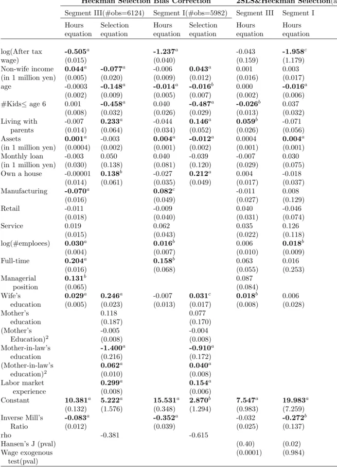
The estimation results are shown in Table 8. For the budget segment III, the estimated wage elasticity for the Heckman two step model is almost the same (-0.50) as the OLS wage elasticity of -0.49 (see OLS7 Table 5). However, the coefficient for the inverse Mill’s ratio is statistically significant at the 1% level. Thus, we could reject the null hypothesis that the selection into labor force is random. For the budget segment I, the wage coefficient only slightly increases from the OLS estimate of -1.28 to -1.24 after applying the Heckman two step procedure. However, we could reject the absence of the sample selection bias at the 1% significance level.
Now, we control for the possible wage endogeneity while controlling for the sample selection bias. This is done by including the the computed inverse Mill’s ratio in the hours worked equation, then applying the 2SLS procedure. This procedure provides a consistent estimate of the coefficients (Wooldridge 2002:567). Table 8 shows the results. For the budget segment III, Hansen’s J test does not reject the validity of the over-identifying restrictions. The wage coefficient drops from the 2SLS estimate of 0.096 (see IV5 in Table
7) to -0.04, though the coefficient is not statistically significant. For the budget segment I, the excluded instruments are not significant determinants of the wage equation when the Heckman sample selection correction term is included in the model. Thus, the model is not identified.
6.
A new estimate of labor supply using a joint
esti-mation incorporating unobserved heterogeneity
Although the 2SLS procedure with Heckman sample selection correction term could control for sample selection into labor force as well as wage endogeneity, we have not taken into account the possibly endogenous selection into different budget segments. Moreover, the large standard errors for the wage coefficients as well as the weak instruments in the 2SLS models hinders the usefulness of the results in policy analysis. Thus, we need more efficient method of estimating the wage elasticity while simultaneously controlling for all the sources of bias discussed so far. For this purpose, we estimate the following model
log(hour)(III)it = β11log(wage)it+ β12Z1it0 + (ρ|1χi{z+ ²IIIit} Error term
) (12)
log(wage)it(III) = α1Z1it0 + γ1Z2it0 + (ρ2χi+ uIIIit ) (13)
log(hour)(I)it = β21log(wage)it+ β22Z
0
1it+ (ρ3χi+ ²Iit) (14)
log(wage)it(I) = α2Z1it0 + γ2Z2it0 + (ρ4χi+ uIit) (15)
Budget segment selection : Bit∗ = α3Z1it0 + γ3Z2it0 + (ρ5χi+ vitB) (16)
Labor f orce selection : I∗
it = α4Z1it0 + γ4Z2it0 + (ρ6χi+ vitL) (17)
Equation (12) is the hours worked equation for the budget segment III, and equation (13) is its corresponding reduced form wage equation. The error terms for both equations are
decomposed into two parts (inside the parentheses). The first part is ρjχi for j=1,2. The
term χi is the unobserved heterogeneity that affects all the equations. The term ρj is the
²III
it and ²Iit, which are assumed to be uncorrelated with any of the explanatory variables.
The covariance between the two error terms is given by Cov(ρ1χi +²IIIit ,ρ2 χi+uIIIit )=ρ1ρ2.
Therefore, the assumption of wage exogeneity for the segment III is equivalent to ρ1ρ2 = 0.
Equation (14) is the hours worked equation for the budget segment I, and equation (15) is the corresponding reduced form wage equation. Similar to the case for the budget
segment III, wage is exogenous if ρ3ρ4=0. Equation (16) is the selection equation between
the two budget segments such that, if B∗
it > 0, the person chooses the budget segment III, and choose budget segment I if otherwise. The correlations of the error terms between
the budget segment selection equation and the hours worked equations are captured by χi
when ρjρ5 6= 0 for j=1,3. If ρjρ5 are not equal to zero for j=1,3, the failure to control for
this non-random selection would introduce a bias in the hours worked equations. Finally, equation (17) is the labor force participation equation where women participate in the labor force if I∗
it > 0. The effect of non-random selection into labor force is captured by χi when
ρ6ρj 6= 0 for j=1,..5.
We estimate all the equations jointly by using a maximum likelihood estimation. In
doing so, we assume that χi ∼ N(0, 1) and all the usual disturbance terms for the hours
worked equations and wage equations (²III,²I,vIII,vI) are independent and distributed
nor-mally. We assume that residual terms for the two selection equations, vB
it and vitL, are independent and follow the logistic distribution. By jointly estimating all the equations, we can control for any correlations among these equations. Thus, this model simultane-ously controls for all the sources of bias discussed so far, namely the wage endogeneity, the endogenous selection between different budget segments, and the self selection into labor force. The likelihood function is in the Appendix.
6.1
Estimation results
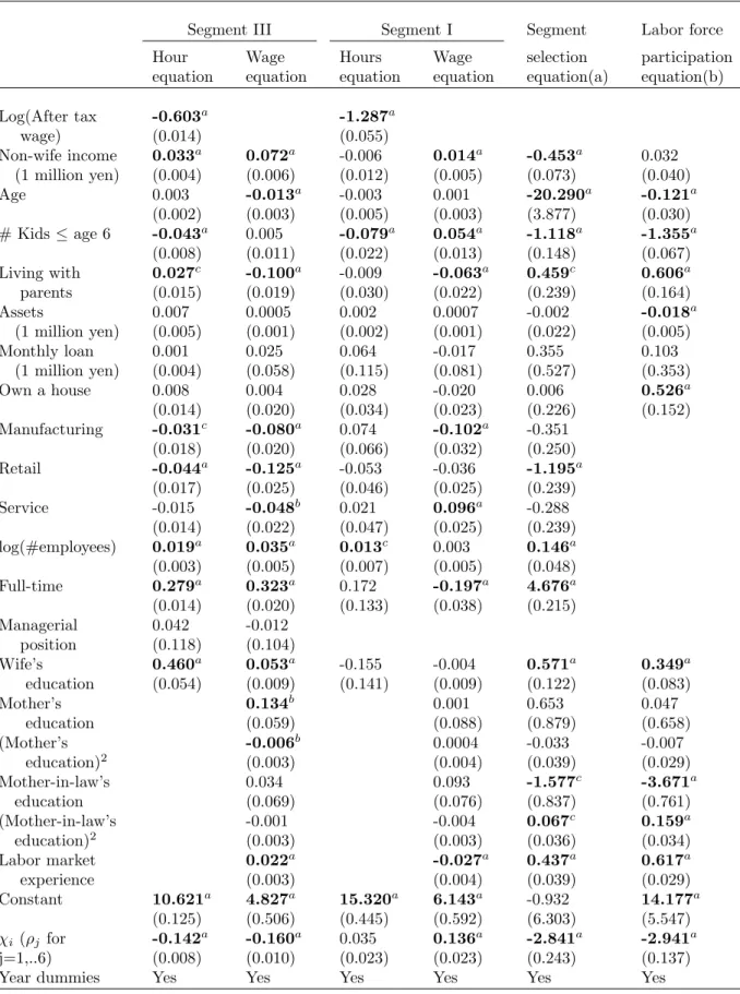
Table 9 shows the results. We impose the common exclusion restrictions for the wage and the selection equations. The exclusion restrictions are the same as the ones used in IV5 in Table 7. First, let us present the results for the budget segment III. The wage elasticity for the budget segment III drops considerably from the OLS estimate of -0.49 to -0.60. Note
that the factor loads for the hours worked equation (ρ1) and the wage equation (ρ2) are
both negative and statistically significant, indicating that the OLS estimate would be biased
upward.11 The factor loads for the budget selection and the labor force selection equations
(ρ5and ρ6) are both negative and statistically significant. The estimated correlation between
the hours worked error term and the budget segment selection error term is 0.571, while it is 0.573 between the hours worked error term and the labor force selection equation error
term.12 Thus, the correlations between the hours worked equation and the two selection
equations are relatively high, which would caused a significant selection bias in the OLS estimate.
A large drop in the wage elasticity is similar to the result for the fixed effect model. The estimated wage elasticity of -0.60 is not far from the fixed-effect estimate of -0.65. However, the wage elasticity for our joint estimation contrasts sharply with the 2SLS wage elasticity of 0.096. One possible reason for this discrepancy is that, while the 2SLS procedure could eliminate both time-invariant and time-varying unobserved heterogeneity, our current model controls only for time-invariant unobserved heterogeneity. However, this discrepancy could also arise from the inefficiency in the 2SLS estimation. Bound et al. (1995) show that when the correlation between the instrumental variables and the endogenous variable is weak, 2SLS estimate is biased in the finite sample. Although our excluded instruments
11Since ρ
1ρ2> 0.
12The correlation between hours worked equation error and the budget segment selection error is given by ρ1ρ5/( p ρ2 1+ σ²2 p ρ2 5+ σv2).
are significant determinants of the wage in the 2SLS model (F-stat=9.48), the test of weak instruments provided by Stock and Yogo (2002) cannot reject the null hypothesis that
the bias in the 2SLS wage coefficient, relative to the OLS bias, exceeds 10.%13 Thus, an
efficient maximum likelihood estimation such as ours may provide a more accurate estimate than the 2SLS. It should also be noted that the statistical control for the endogenous selection between the two budget segments as well as other sources of bias are likely to have contributed to this discrepancy as well.
For the budget segment I, the estimated wage elasticity is -1.28 which is almost the same as the OLS estimate. The factor load for the hours worked equation is small (0.015) and statistically insignificant. Thus, the effects of the unobserved heterogeneity through the wage equation and the two selection equations would have little impact on the hours worked equation, suggesting that the wage is not endogenous for the budget segment I. We cannot reject the null hypothesis that the wage elasticity is smaller than -1. This suggests a possible ‘income adjustment behavior’ of wives in this budget segment.
Other coefficients are of interest. The effect of age on the hours worked is positive for the budget segment III (0.003) while it is negative for the budget segment I (-0.003), though both of the coefficients are not statistically significant. The results for the budget segment selection equation and the labor force participation equation indicate that, as age increases, (i) the likelihood of choosing the budget segment I increases (the wife becomes dependent on the husband’ income) and (ii) the likelihood of being out of labor force increases. These results indicate that the age-hours worked profile has a hump shape, the shape similar to the well-known M-shaped age-labor force participation profile for Japanese women; At a relatively young age, women are in the budget segment III where the effect of age on the hours worked is positive. Then these women move to the budget segment I where the effect
13The test statistic (Kleibergen-Paap F statistic) is 9.49 while the the critical value for the 10% IV relative bias is 10.83
of age is negative.
Living with parents has a positive and statistically significant effect on the labor force participation, confirming Sasaki’s (2002) finding. However, at the 5% significance level, living with parents does not have significant effects on the hours worked for both of the budget segments as well as on the selection between the budget segments. The effect of the number of kids on the hours worked is twice more negative for the budget segment I (-0.08) than for the budget segment III (-0.04). This could be due to the fact that most of the women in the budget segment I hold a part-time job where working hours are considerably more flexible than a full-time position. The more negative effect of young children on the hours worked for the segment I is also consistent with Ueda’s (2007) findings that the utility losses from childcare in a life-cycle childbearing model is greater for part-time workers than for full-time workers. The greater utility losses for part-time workers could have resulted in a greater decrease in the hours worked for the segment I in our data.
In sum, labor supply behavior of women in the two budget segments are notably differ-ent. Wage elasticity is twice more negative for the women in the budget segment I (-1.28) than for women in the budget segment III (-0.60). We cannot reject the null hypothesis that the wage elasticity is smaller than -1 for those in the budget segment I, suggesting a possible ‘income adjustment behavior’ for the women in this budget segment. The sign of the effect of age on the hour of work is opposite for the budget segment III and I.
7.
Conclusion
We first examined the sensitivity of the wage elasticity of Japanese married women to various economic and statistical assumptions by using a sample from the Japanese Panel
Survey of Consumers. We then provided a new estimate of the female labor supply that
endogenous selection between different segments of the non-linear and often discontinuous budget constraint. We found that the OLS estimate of the wage elasticity substantially drops when job related characteristics are included in the model. The assumption of wage exogeneity is rejected. We found that the wife’s labor market experience is a valid excluded instrument while the wife’s education should be directly included in the hours worked equation in the 2SLS procedure. This finding validates most of the model specifications in the previous studies in Japan that utilize instrumental variable methods. The assumption of no-sample selection bias is rejected, though the correction of the bias in the Heckman two step procedure has little impact on the estimated wage elasticity.
Our new estimate of labor supply shows that there are notable differences in the labor supply behavior of women who choose different segments of the budget constraint. In particular, the wage elasticity of women who choose the budget segment I (annual income less than 1.03 million yen ceiling) is twice more negative (-1.28) than the women who choose the budget segment III (annual income greater than 1.41 million yen ceiling) (-0.60). In the case of the budget segment I, we cannot reject the null hypothesis that the wage elasticity is smaller than -1, suggesting that these women may be adjusting their hours of work so that their income does not exceeds the 1.03 million yen ceiling. The effect of the number of kids on the hours worked is also twice more negative for the budget segment I (-0.08) than for the budget segment III (-0.04). The effect of age on the hours worked is positive for the women in the budget segment III while it is negative for the women in the budget segment I. Younger women are more likely to choose the budget segment III while older women tend to choose the budget segment I. These results indicate that age-hours worked profile for Japanese married women has a hump-shape, a shape similar to the well-known M-shaped age-labor force participation profile for Japanese women. Our maximum likelihood estimation improved upon the previous literature in that it simultaneously controlled for
various sources of bias discussed in the literature, and that it provided a much more efficient estimate of the wage elasticity than the 2SLS procedure.
References
Abe, Yukiko, 2009. The Effects of the 1.03 Million Yen Ceiling in a Dynamic Labor Supply Model. Contemporary Economic Policy, April, Vol. 27, Issue 2, p147-163,
Abe, Yukiko and Fumio Otake. (1995). “Zeisei Shakai Hosho Seido to Part-Time Roudou-sha no Roudou Kyoukyuu Koudou (Tax and Social Security System and Part-time Workers’ Labor Supply Behavior), Kikan Shakai Hosho Kenkyu, Autumn, Vol. 31, No. 2, pp. 120-134 (in Japanese).
Akabayashi, Hideo, 2006. The Labor Supply of Married Women and Spousal Tax Deduc-tions in Japan. Review of Economics of the Household, Issue 4, pp. 349-378.
Bound, John; David A. Jaeger; and Regina Baker, 1995. Problems with instrumental variables estimation when the correlation between the instruments and the endogenous explanatory variable is weak. Journal of American Statistical Association, 90, pp. 443-450
Borjas, George J, 1980. The Relationship between Wages and Weekly Hours of Work: The Role of Division Bias. The Journal of Human Resources, Vol. 15, No. 3, Summer, pp. 409-423.
Debroux, Philippe, 2003. Human Resource Management in Japan: Changes and
Uncer-tainties, Gower Publishing Co.
Hansen, Lars P, 1982. Large Sample Properties of the Generalized Method of Moments Estimators. Econometrica, 50, 1029-1054.
Hausman, Jerry A, 1980. The Effects of Wages, Taxes, and Fixed Costs on Women’s Labor Force Participation. Journal of Public Economics, 14, pp. 161-194.
Hayashi, Fumio, 2000. Econometrics. Princeton: Princeton University Press.
Heckman, Jamese, 1979. Sample Selection Bias as a Specification Error. Econometrica, 47, pp. 153-161.
Hill, Anne, 1989. Female Labor Supply in Japan: Implications of the Informal Sector for Labor Force Participation and Hours of Work. The Journal of Human Resources, Vol. 24, No. 1, Winter, pp. 143-161.
Ihori, Toshihiro, Ryuta Ray Kato, Masumi Kawade, and Shun-ichiro Bessho, 2006. Public Debt and Economic Growth in an Aging Japan. K. Kaizuka and A. O. Krueger eds
Tackling Japan’s Fiscal Challenges, Palgrave.
Kato, Ryuta Ray, (2002) Government deficit, public investment, and public capital in the transition to an aging Japan. Journal of the Japanese and International Economies, Vol. 16, pp. 462-491.
Kuroda, Shoko and kaoru Yamamoto, 2008a. Ijitenkan no Roudou Kyoukyuu Dansei-chi (Frisch dansei-chi) no Keisoku. (The Estimation of the Intertemporal Labor Supply Elasticity (Frish-elasticity)). Mita Shougaku Kenkyuu, June, Vol. 51, No. 2, pp. 77-92 (in Japanese).
Kuroda, Shoko and kaoru Yamamoto, 2008b. Estimating Frish Labor Supply Elasticity in Japan. Journal of Japanese and International Economies, Vol. 22, pp. 566-585. MaCurdy, Thomas E, 1981. An Empirical Model of Labor Supply in a Life-Cycle Setting.
The Journal of Political Economy, Vol. 89, No. 6, December, pp. 1059-1085
Moffit, Robert, 1986. The Economics of Piecewise-linear Budget Constraints. The Journal
of Business and Economics Statistics, 4(3), pp. 317-328.
Mroz, Tomas A, 1987. The Sensitivity of an Empirical Model of Married Women’s Hours of Work to Economic and Statistical Assumptions. Econometrica, Vol. 55, No. 4, July, pp. 765-799.
National Institute of Population and Social Security Research, 2008. Population Projections for Japan: 2006 - 2055 December 2006. National Institute of Population and Social
Security Research.
Nakamura, Jiro and Atsuko Ueda, 1999. On the Determinants of Career Interruption by Childbirth among Married Women in Japan. Journal of the Japanese and
Interna-tional Economics, 13, pp. 74-89.
Oishi, Akiko, 2003. Yuu Haiguu Sha Josei no Roudou Kyoukyuu to Zeisei Shakai Hoshou Seido (Married women’s labor supply and the Tax-Social Security System). Kikan
Shakai Hoshou Kenkyuu, Vol. 39, No. 3, Winter, pp. 286-305 (in Japanese).
Sasaki, Masaru, 2002. The Causal Effect of Family Structure on Labor Force Participation among Japanese Married Women. The Journal of Human Resources, Vol. 37, No. 2., Spring, pp. 429-440.
Stock, James H, and Morihiro Yogo, 2002. Testing for Weak Instruments in Linear IV Re-gression. National Bureau of Economic Research Technical Working Paper 284, Oc-tober. Downloadable at http://www.nber.org/papers/t0284 (Accessed July 30 2009). Ueda, Atsuko, 2007. A Dynamic Decision Model of Marriage, Childbearing, and Labour Force Participation of Women in Japan. Japanese Economic Review, Vol. 58, Issue 4, December, pp. 443-465.
Wooldridge, Jefferey M, 2002. Econometric Analysis of Cross Section and Panel Data. The MIT Press Cambridge, Massachusetts
Table 1: National Income Tax Brackets in 2002
Taxable Income Range Marginal tax rate (%) in 1000 yen (y)
1 ≤ y < 3,300 10% 3,300 ≤ y < 9,000 20% 9,000 ≤ y < 18,000 30%
18,000 and more 37%
Tax schedule has been changed in 1995 and 1998. We took into account these changes when we computed the after tax wage rate.
Table 2: The Employee Tax Deduction Schedule in 2002
Gross Income Range Total Deduction
in 1000 yen (y) (Basic + Employer deduction)
1 ≤ y < 1,625 1,030 1,625 ≤ y < 1,800 0.4y+380 1,800 ≤ y < 3,600 0.3y+560 3,600 ≤ y < 6,600 0.2y+920 6,600 ≤ y < 10,000 0.1y+1,580 10,000 and more 0.5y+2,080
Tax deduction schedule was changed in 1995 and 2003. We took into account these changes when we computed the after tax wage rate.