An Approach for the Optimal Production Rate of a Single Product System with Dynamic Demands

(1)

Society of Japan

Vol. 29, No. 3, September 1986

AN APPROACH FOR THE OPTIMAL PRODUCTION RATE

OF A SINGLE PRODUCT SYSTEM

WITH DYNAMIC DEMANDS

Chang Sup Sung M. H. Park

Korea Advanced Institute of Science & Technology (KAIST)

(Received October 11, 1983: Final February 3,1986)

Abstract The optimal production rate (production capadty) for a single product system with some deterministic dynamic demands is considered. Under a linear-additivity assumption on the associated cost information, the existence of the optimal solution for production capacity is verified. For the model, two solving techniques (point-wise computation and L.P. approaches) are developed for both uniilled-demand handling cases of lost-sales and backlOgging, with which example problems are tested to show the superiority of the point-wise computation ap-proach to L.P. apap-proach.

1. Introduction

Given a finite time horizon

[O,T]

partitioned into several time-periods (time-intervals) during which the period--wise demands are variant accordingly, the optimal capacity determination of a production system is practically of great importance in investment view. Furthermore, when the operation of the system at a fixed production rate, say A" through the time horizon is con-sidered, the associated inventory systems should be accounted for to derive the optimal investment decision giving rise to an optimal value A*

Florian and Klein [2] and Lambrecht et al. [5] have studied the problems of production scheduling with the allowance of the period-wise different pro-duction quantity, given the known demands. Their works were based on a given system with bounded capacities, so that some of its production schedules may include certain idle periods.

By the way, from the standpoint of the system utilization and cost caused from production changes, the operation of a system at a fixed production rate

(2)

178

c.

S. Sung & M. H. Park

production system for a commodity. Then, the system operation schedules would be studied with respect to its full utilization. This problem can be inter-preted as the problem of finding a schedule for the ssytem to be operated at a constant (fixed) production rate and without any idle period.

For this study, both cases of backlogging and lost-sales are to be treated for the optimal production rate A* at which the total profit through the time horizon is maximized.

In the following section, a production rate decision model for both cases of lost-sales and backlogging is developed. In fact, a more general problem including this problem as a special case can be formulated as a linear pro-gramming problem and hence can be solved efficiently. Therefore, for the model, the optimal solution algorithms are proposed in L.P. and point-wise computation approaches. It is then shown that for the special case the point-wise computation algorithm is more efficient than L.P. algorithm.

2. Total Profit Model

The model dealt with in this section is of determining the optimal capa-city of a production system corresponding to a sequence of the deterministic future demands. For its analysis, a total profit through the time horizon is defined as follows;

Total Profit

(TR)

(quantity sold) x (unit price) + (salvage value) - (inventory holding cost) - (shortage cost) - (initial investment) - (manufacturing cost).

Let N be the total number of periods over the time horizon and fit be the

manufacturing cost for a product in period t. Then, the first term of TR is

N

represented as

I

UtS_t, where St is the quantity sold during period t and Ut t=l

is the unit price of a product. Salvage value is composed of two elements, one for the initial investment and the other for the products salvaged. The latter is denoted by kI

N+, where k is the salvage value of a product (k -< fi ) t and IN+ is the positive inventory. The former is represented by rCA estimated at the end of period N, where r (JrJ < 1) is the salvage value conversion rate and CA is the initial investment for the system which is assumed to be linearly proportional to A.

Let h

t be holding cost per unit held from period t to t+1 and TIt be

shortage cost. Under the assumption that inventory holding costs are linearly proportional to the net inventory at the end of priod t (denoted by It)' TR is

(3)

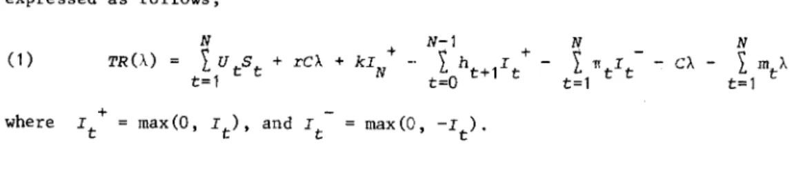
expressed as follows; N N-1 N N (1) TR(A)

tu

_{tSt + reA +} + tI Oh t +1I t +

I

TItI t - CA -

I

lntA = _kIN

-t=l t=l t=l

where _It+ max(O, _It)'and _It max (0, -It)'

3. Optimal Solution Search: Lost-Sales Case

In this section, a model will be analyzed for which the unsatisfied demand for a period assumes lost. Then, St and 1t can be expressed as follows:

denoting by d

t the demand during period t,

(2) _min(d +

t, A + max(It_1, 0»

=

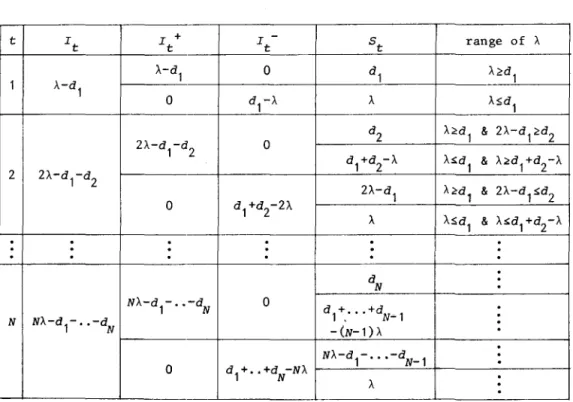
min(dt, A + It-1 )

Eqs.(2) and (3) depend piece-wisely upon A. Such dependency is summarized in Table 1.

Table 1. It and St Piece-Wisely Depending upon A.

+

-of A t _It _It _It _St _range --r--- -A-d 1 0 d1 A2d1 1 A-d 1 --0 d 1-A _- A A~d1 2A-d 1-d2 0 d2 A2d1 & 2:\:<!d1+d2 ZA-d 1-d2 --0 d

1+d2-2\ 2A-d1 A2: d1 & 2A~d1+d2 2

A-d

2 0 d2 A~d1 & A2d2

A-d 2

0 d

2-A A A~d1 & A~d2

·

_·

·

· ·

·

_·

-- -

·

--NA-d 1-· .-dN 0 dN NA-d 1-· .-dN -0 d₁+·· .dN--NA NA-d 1-· .-dN-1

--·

·

N

·

.-A-d N 0 dN A-d N 0 dN-A A

(4)

-180

c.

S. Sung & M. H. Park

Now, it will be shown that TR is a piece-wise affine function of A.

Theorem

1. The function TR is a piece-wise affine function of A and its slope changes occur at the points, d₁, d₂,···, dN' (d₁+d₂)/Z, ... , (d_N_₁+d_N)/2,

(d₁+d₂+d₃)/3, ... , (dN_2+dN_l+dN)/3, ... , (d₁+· .+dN)/N.

Proof:

From Table 1, it is seen that It , I t and St for t=1,2, ..• ,N + are piece-wise linear functions, respectively, depending upon the ranges of

N-l N N

A. This implies that

I

h_t+₁I_t+,

I

TItI_t- and

r

UtS_t are piece-wise linear

t=O t=l t=l

functions. Meanwhile, the rest part of the function TR is also a linear func-tion of A. Therefore, TR is a piece-wise linear function of A whose slope changes occur at the boundary points given above.

For example, consider the case of "N

=

1". Then, the two possible dis-tinct ranges (intervals) of A are in the set {O~A~dl' dl~A}. Over each range in the set, TR(A) is defined as follows:

(a) For the range dl~A;

TRa(A)

=

(rc-c-m₁+k)A + (U₁d₁-kd 1), (b) For the range O~A~dl;

TRb(A) = (rc-c-m₁+u₁+TI₁)A - TI₁d₁,

where TR.(A) denotes the objective function defined over the range i (i=a,b). ~

These two functions, TRa(A) and TRb(A) , show that each of them is a linear function defined over its associated range (interval), and further that they are equal at the point A

=

d

1•

Also, consider the case of "N

=

Z". Then, all the demands, d

1 and d2, can be ranked as d(1)~d(2) in their nondecreasing order, where d(i) denotes the ith smallest value. Thereupon, the associated range set can be defined as

{O~A~d(l)' d(1)~A$(d(1)+d(2»/2, (d(1)+d(2»/2~A}. Now, assume without loss of generality that dl~d2' Then over each element in the range set {O~A$dl'

dl~A~(dl+d2)/2, (dl+d2)/2~A}, TR(A) is defined as follows:

(a) For the range O!>A!>d 1;

TRa(A)

=

(rc-C-ml-m2+ul+u2+TI1+TI2)A - _{(TI 1d1+TI 2d2),} (b) For the range dl~A~(dl+d2)/2;

TRb(A) = (rC-C-ml-m2+2U2-h2+2TIz)A + (uldl-u2dl+h2dl-1T2dl-TI2d2)'

(c) For the range (dl+d2)J2~A;

(5)

This also shows that each of the three functions is a linear function, and further that TRa(A) and TRb(A) are equal at

A

=

d

"

and TRb(A) and TRc(A) are equal at _{(d , +d2) /2. These imply that 'l'R is a piece-wise affine function} de-fined over the whole domain of A, O~A.

Likewise, in general, N demands d

1,dZ"'" and dN can be ranked as

d(1)$d(2)$ ... $d(N) in their nondecreasing order. It follows that the whole domain of A (O~A) can be decomposed into the distinct intervals of whose boundary points are in the set {O,d" ... ,dN,(d,+d2)/2, ... ,(dN_,+dN)/2, ... ,

(d,+d2+d3)/3, ..• ,(d,+dZ+ •.• +dN)/N}. Then, it can be seen that over each of these intervals, TR is defined as a flinear function of A, and further defined over the whole domain of A as a piece-wise affine function. This completes the proof.

The results of Theorem 1 lead to Theorem 2 which shows the existence of the optimal solution.

Theorem 2.

The function TR has the maximum value at either 0 or one of the boundary points resulted from Theorem 1.

Proof:

From the piece-wise affinity, TR(A) may have local maximums at the boundary points. Therefore, it is sufficient to check the values of A in the ranges outside the smallest and the greatest boundary points.

If A is in the range beyond the greatest boundary points, St=d t,

fi

N-1 I/=tA-d , - ... -dt , It-=O for t=1,2, ... ,N. Thence, TR(A)= A(rC-C-

L

m

t-

It

ht+1 t-1 t=1

fi

N-1

+ NK) + constant, which decreases as

A

increases, because (rC-C-

L

m -

I

t h

t=1 t t=O t+1

+ NK) < O. So, the local maximum of TR(A) over the range is attained at the greatest boundary point.

Meanwhile, if

A

is in the range below the smallest boundary point, St=A, It+=O and It =dt-A for t=1,2, ... ,N. Thence,

N N N

TR(A)

( I

Ut + rC - C - ~ m + ~ TIc)A + constant.

t=l t=l t t=l 1:

This implies that, as A decreases, TR(A) decreases or increases depending upon the coefficient of

A.

Hence, the local maximum over the range is attained at either the smallest point or O.

Thus, the proof is completed.

A solution algorithm, PWA1(abbreviation of point-wise computation ap-proach 1), is then suggested based on Theorems 1 and 2.

(6)

182

c.

S. Sung & M. H. Park Algorithm PWA1

Step Compute values of (d

1+d2)/2, ... , (dN_1+dN)/2, ... , (d1+d2+d3)/3, ... , (dN_2+dN_1+dN)/3, ... , (d₁+ .•. +d_N)/N (Let them be Pi (i=l, 2, ... ,N(N+1)/2+1) including d

1, ... ,dN and 0) Step 2 Compute TR(P_i) for each Pi' where

Step 3

I =I+ + P. - d t t-1 ~ t St=min(dt , Pi +I:- 1)

Compare the values of TR(P.) and find the optimal value

A*

~

maximizing TR such as A*={P_k; TR(Pk)~TR(Pi)' ¥i}

Now, consider the computational complexity of Algorithm PWA1. When the order of computation rather than the detail number of computations is taken into account as the measure of complexity, the algorithm is of order N 3 , which is proved in Lemma 1.

Lemma 1.

Point-wise approach is 0(N3₎ _{for the lost-sales case.}

Proof:

The number of points to be computed is the number of boundary points for the intervals of A and zero point, and so N+(N-1)+ ..• +1+1=N(N+1)/2+1.

+

-Given a boundary point of A, values of It (It) and St are obtained from iterative computation at each partitioning point of time horizon [0,

T],

and so the number of iterations is N.

Thus, the number of computations for optimal

A*

is [N(N+1)/2+1]N=N2(N+1)/ 2+N. This completes the proof.

The algorithm is now illustrated with a numerical example with N=4. Example 1

Assume that the required informatoin is given as follows; d₁=3, d₂=1, d₃=4, d₄=2, N=4, TIt=O.S, h_t=0.2, ID t=2, Ut=3.3 for t=1, ... ,4, c=4, r=O.l, k=2.S. Then, P 1=3,P2=1, P3=4, P4=2, PS=2, P6=2.S, P7=3, PS=S/3, Pg=7/3, P10=2.S, P11=0. So, TR(P 1 ) TR(P7) = 2.6 TR(P2) -1.4 TR(P 3) -0.2 TR(P4) TR(PS) 2.0 TR(P 6) TR(P10) 3.0S TR(PS) 2.9 TR(P_{g )} 2.7 TR(P 11) = -S

A*

2.S

(7)

Our problem can also be handled in linear programming (LP) approach. From Eqs. (1), (2) and (3), the problem can be formulated in LP as follows:

maximize A + s. t.

-

_Il ₊_Il d 1 2S 1

-

A + + Il + Il d 1 A + _{I t -} ₁+

-

It + + It d t 2S t - A + +

-

_{I t - 1} + It + It d t + St 2 0, It ~ 0, _It: ~ 0, ¥t A ~ 0.

Observe that the vector of constraint coefficients for I

t+ is linearly dependent with that of I

t- This meanE that I t + and I t cannot both be in a basic solution, and hence that the conE,traint It + 'I

t- = 0, implied by the

definition of on-hand inventory and backorders, is automatically satisfied and does not have to be represented explicitly in the model.

4. Optimal Solution Search: Backlogging Case

Another model shall be analyzed for which unsatisfied demands can bE! satisfied later. In this case, St and It are expressed as follows:

(4) min [max(I

t_1, 0) + A, dt-min(It_1, 0)]

min (5)

Eqs.(4) and (5) also depend piece-wisely upon

A.

Such dependency is summarized in Table 2.

The function TR, even i f it is nevdy defined with St and It given in Eqs.(4) and (5), can be proved to have similar solution properties to those in the lost-sales case. The properties are stated in Theorems 3 and 4.

(8)

184 C. S. Sung & M H. POTk

Table 2. I t and St Piece-Wisely Depending upon A

t _It I + t It

-

St range of A A-d 1 0 d1 A~d1 1 A-d 1 0 d 1-A A ASd1 d

2 A~d1 & 2A-d1~d2

2A-d

l-d2 0 _d

l+d2-A A,;:d1 & A~dl+d2-A 2 ZA-d

1-d2

ZA-d

1 A~dl & 2A-d1~d2

0 d 1+d2-ZA A ASd l & A,;:dl+d2-A

·

_·

d N

·

NA-d l-· .-dN 0 _{d 1+:·}_{.+dN- 1}

·

N NA-d l-· .-dN -(N-l)A

·

NA-d_l-·· _{.-dN- l}

·

0 d_l+· .+dN-NA

·

A

·

· Theorem 3.

The function TR is a piece-wise affine function of A whose

slope changes occur at the points d

l, (dl+d2)/2, (dl+d2+d3)/3, ... , (d₁+·· .+dN)/N.

Proof:

The proof is straightforward when the proof steps of Theorem 1

are followed by use of Table 2.

Theorem

4.

The function TR has the maximum value at either 0 or one of

the boundary points resulted from Theorem 3.

Proof:

It is easily proved by use of the results of Theorem 3 when the

proof steps of Theorem 2 are followed.

Based on the results of Theorems 3 and 4, a solution algorithm, PWA2 (point-wise computation approach 2), for the backlogging case is then devel-oped.

Algorithm PWA2.

Step 1 Compute the values of d

l, (dl+d2)/2, (dl+d2+d3)/3, •.. , (d

(9)

respectively, with P =0)

N+l

Step 2 Compute TR(P

i) for each Pi' where It

=

_{I t - 1}+ Pi - d_t

St = min(I:__f+ Pi' d_t +

I~_l)

Step 3 Same as step 3 of PWA1.

As done for Algorithm PWA1, when the order of computation is considered as the measure of computational complexlty, Lemma 2 shows that Algorithm PWA2 is of order N2, which can be proved in the same way as for Lemma 1.

Lemma 2.

For the backlogging case, point-wise approach is 0(N2) .

Example 2 is presented for illustrating Algorithm pWA2. Example 2

The required data are the same as those of Example 1 except 1T

t=0.3 for t=l, 2, 3, 4.

Then, P

1=3, P2=2, P3=8/3, P4=2.S, PS=O and so, TR(P1) = 2.6, TR(P2) -3.3,

T~(P3) = 3.36, TR(P

S

)

= 3.S, TR(P

S

)

= -7.S, 1-* = 2.S

From Eqs. (1), (4) and (5), the baeklogging problem is also formulated into LP as follows: I- + s.t. _I1 + _Il d 1 2S 1 I-+ d 1 + _I1 + _I1 I- + I + + t_1 It I t - 1 + It dt + + 2S t I- It_1 + It It_1 + It dt t=2, ... ,N 0, + :2 0, 0, ¥t. l- D St :! It -[t :! :!

5. Comments on Computational Complexity (Point-wise Computation vs. LP)

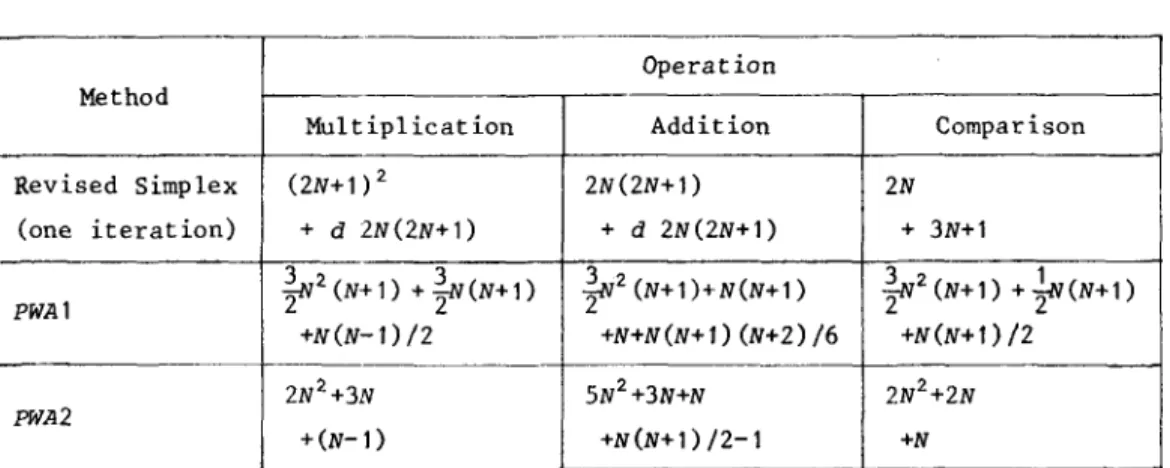
Bazaraa [1] illustrated the number of operations required during an iteration in solving LP problem by the revised simplex method. Bazaraa's result with the number of operations required for the point-wise computation approach is listed in Table 3, where LP is based on one iteration but

(10)

point-186

c.

S. Sung & M. H. Park

wise approach is based on the whole computation, and d is the density of non-zero elements in the constant matrix.

Table 3. LP vs. Point-Wise Computation Approach (N periods)

Operation Method

Multiplication Addition Comparison

Revised Simplex (ZN+1)

2

_ZN(ZN+1) _ZN (one iteration) + d 2N(ZN+1) + d ZN(ZN+1) + 3N+1 PWA1

}2

(N+ 1) + }(N+1)

}2

(N+1 )+N(N+1)

}2

(N+1) + ¥(N+1) +N(N-1)/Z +N+N(N+l) (N+Z)/6 +N(N+1) /Z ZN2+3N SN2+3N+N 2N2+ZN PWAZ +(N-l ) +N(N+ 1) /Z-1 +N

Garey and Johnson [3] have stated that with reference to Klee and Minty [4], the simplex algorithm for LP has exponential time complexity. However, in practice, the simplex method has an impressive record of running quickly. Meanwhile, there is no general conclusion for the number of iterations required

for finding the optimal solution in the simplex method. Therefore, it is difficult to conclude which approach is the more efficient one, in general, of two.

Several numerical examples are solved on Cyber 174 to make a computational efficiency comparison in CPU time between PWA's and LP approaches, with the variations of cost coefficients of

A

and of the planning horizon N, the results of which are listed in Table 4 and 5. In Table 5, CA represents the function

N

of C d~fined as C

= C -

rC + ~ m. Table 4 shows CPU time requirements for

A t=l t

finding optimal solutions to each of the problems generated by varying the +

information of Ut' TIt ' TIt '

k=1.5 and mt=Z.O. And Table

h

t and N, for the fixed data of C=4.0, r=O.l,

5 shows such CPU time requirements for the

prob-+

lems generated for the fixed data of U

t=3.3, TIt =0.3, TIt =0.5, ht=O.Z, k=I.S and mt=Z.O.

(11)

Table 4_ Computation Time Comparison in CPU on Cyber 174 between

PWA's and LP with c=4.0, r=0.1, k=1.5 and m

t=2.0. Data Ut '!Tt ht 3.3 0.5 0.2 (0.3) 0.8 0.2 (0.6) 0.4 1.1 0.4 (0.9) 3.3 1.1 0.6 (0.9) 3.0 0.5 0.2 (0.3) 0.8 0.2 (0.6) 0.4 1.1 0.4 (0.9) 0.6 periods 4 12 24 4 12 24 4 12 24 4 12 24 4 12 24 4 12 24 4 12 24 4 12 24 4 12 24 4 12 24 1 ost-sales case (sec. ) F 'WA1 0 0

o

0

o

0

o

0

o

-0

o

0 0 0

o

-o

o

-o

o

.058 .089 .215 .056 .086 .220 .058 .088 .221 .058 .084 .216 .058 .083 .221 .056 .083 .208 .058 .085 .213 .055 .085 .213 .057 .086 .214 .057 .082 .220 LP --0.929 1.156 1.518 0.902 1.164 1.509 0.903 1.146 1.509 I 0.905 _1.128 1.523 0.910 1.142 1.533 0.916 1.144 1.512 0.920 1.131 1.549 0.931 1.120 1.529 0.913 1.128 1.539 0.898 1 .121 1.572 ' -+

(Note: Values in parentheses indicate IT

t values). backlogging case (sec.) PWA2 LP 0.056 0.933 0.082 1.268 0.204 1.710 0.055 0.917 0.083 1.263 0.205 1.713 0.056 0.911 0.085 1.261 0.205 1.710 0.058 0.907 0.083 1.244 0.207 1.743 0.056 0.912 0.083 1.254 0.213 1. 712 0.055 0.917 0.086 1.293 0.212 1.699 0.057 0.913 0.084 1.271 0.210 1.717 0.056 0.911 0.083 1.274 0.202 1.706 0.056 0.911 0.089 1.248 0.213 1.711 0.056 0.907 0.082 1.274 0.208 1.715

(12)

188

c.

S. Sung & M. H. Park

Table 5. Computation Time Comparison in CPU on Cyber 174 between PWA's and LP with U

t=3.3, TIt+=0.3, nt-=0.5, r=O.l, h

t=0.2, k=1.5 and IDt=2.0.

Data lost-sales case back logging case

(sec. ) (sec.)

C CA periods PWA1 LP PWA2 LP

4.0 11.6 4 0.058 0.929 0.056 0.933 27.6 12 0.089 1.156 0.082 1.268 51.6 24 0.215 1.518 0.204 1. 710 100.0 98.0 4 0.052 0.942 0.051 1.013 114.0 12 0.080 1.555 0.080 1.641 138.0 24 0.211 2.529 0.204 2.611 200.0 188.0 4 0.051 0.948 0.052 1.051 204.0 12 0.080 1.558 0.077 1.644 228.0 24 0.216 2.726 0.206 2.749

Tables 4 and 5 show that given three N values 4, 12 and 24, in our PWA approaches CPU time does not vary with the cost coefficients of A, while it greatly depends on the variations of planning horizon N. However, LP approach spent ten times the CPU time in searching each associated optimal solution, even if it is less sensitive to the variations of N values than PWA approaches. Furthermore, Table 5 shows that as C increases, the CPU time requirement in LP approach also increases.

In conclusion, for problems with N not large, our PWA approach is effi-cient more than ten times in comparison with LP approach. In particular, when C is greater than 200 and N is less than 12, the superiority of PWA to LP approach in computational efficiency becomes more conspicuous. We further claim that PWA approach could be practically appreciated in its application to fairly large planning problems such as monthly production planning over five years, weekly production planning over season, etc. In fact, under a variety of uncertain industrial environments, forecasted demands will be meaningful in product management only over a certain limited time interval, so that the problem size parameter, the number of time-periods N, of our problem won't be large. Therewith, it can be argued that with reference to the computational complexity comparisons shown in Tables 3, 4 and 5 the point-wise computation approach is superior from the practical application view, because the study objective of determining the optimal product rate A* is based on the forecasted future demands.

(13)

Remarks:

It is noted that the above piece-wise computation approach can also be directly applied for searching the optimal solution of A to the piece-wise total profit function which consists of convex functions defined over each interval of

A.

This occurs when each cost function with respect to inventory holding and shortage and initial investiment is assumed concave in I

t+, It

and A, respectively. In fact, the maximum value of a convex function for an interval is attained at one of the boundary points of the interval.

As shown in Algorithms 1 and 2, for the specific problem the computational complexities in PWA's depend on the number of horizon periods rather than the coefficient of A. If we consider a situation in which the conditions k!:mt for all t are removed and rather a production capacity restriction is placed as an upper bound of A, then a maximum valw~ of TR would also be guaranteed, since the capacity bound should be included as a boundary point.

6. Conclusion

As shown through this work, two searching approaches are suggested for finding the optimal production rate for a system, the total profit function of which is a piece-wise affine (linear or convex) function, given a sequence of deterministic demands.

The importance of this study is placed on the case in which the produc-tion management is highly dependent upon the optimal utilizaproduc-tion of facilities. It may also be of practical interest to some production systems, of which the change of production rate is too costly.

From the efficiency comparison between the two approaches, the point-wise computation approach seems to be advantageous in its applying to real problems.

Certain production systems with stochastic demand processes are currently under investigation as an extension of this work.

Acknowledgment

The authors are grateful to Mr. W.S. Lee for his help with computer calcu-lations and also wish to thank the referees for their numerous valuable sugges-tions and comments contributed to the improvement of the paper.

(14)

190

_c.

S. Sung & M. /I. Park

References

[1] Bazaraa, M. S., and Jarvis, J. J.: I,inear Programming and Network Flows, Wiley, New York, 1977.

[2] Florian, M., and Klein, M.: Deterministic Production Planning with Concave Costs and Capacity Constraints. Management Science, Vol.18 (1971), 12-20. [3] Garey, M. R., and Johnson, D. S.: Computers and Interactibility - A Guide to the Theory of NP-Completeness, W. H. Feeman and Company, San Francisco, 1979.

[4] Klee, V., and Minty, G. J.: How good is the simplex algorithm in Inequali-ties III, edited by O. Shisha, Academic Press, New York, 1972.

[5] Lambrecht, M., and Vander Eecken, J.: A Capacity Constrained Single

Facility Dynamic Lot-Size Model, European Journal of Operational Research, Vol.2 (1978), 132-136.

C. S. SUNG: Department of Industrial Engineering, Korea Advanced Institute of Science & Technology, P.O.Box 150, Cheongryang, Seoul, Korea.