On the Computational Efficiency of Branch -and- Bound Algorithms

Society of Japan

Vol. 20, No. I, March, 1977

ON THE COMPUTATIONAL EFFICIENCY

OF BRANCH-AND-BOUND ALGORITHMS

TOSHIHIDE IBARAKI, Kyoto University

(Received June 4, 1976; Revised September 16, 1976)

Abstract. The behavior of the number of partial problems T(A) which are decomposed in a branch-and-bound algorithm A (T(A) may be taken as a measure for the computational efficiency of A) is investigated in a fairly general setting. The first result is that the mean number f(n) of T(A) when A is applied to problems of size n grows at least as fast as exponentially with n, under relatively mild conditions, if A uses only the lower bound test as most of the conventional branch-and-bound algorithms do. Then it is pointed out that a possible way to avoid this exponential growth is to use the dominance test together with the lower bound test. The dominance test is also interesting from the view point of unifying a wide variety of algorithms as branch-and-bound.

These points are exemplified by the well known Dijkstra algorithm for the shortest path problem and the Johnson algorithm for the two-machine flow-shop scheduling problem, for which f(n)

:s:

n-1 holds by virtue of the dominance test.

1.

Introduction

Branch-and-bound is a computational principle used to solve various com-binatorial optimization problems, in particular those which are not so nicely structured as to permit very efficient algorithms. For many "difficult" problems, such as the integer programming problem, the traveling salesman problem and various scheduling problems, branch-and-bound is reportedly the only practical approach.

As is well known, e.g. [1, 10, 11, 21, 23, 25, 27}, the underlying idea of branch-and-bound is to decompose a given minimization problem

Po

into more than one partial problem of smaller size. The decomposition is repeatedly applied to the generated partial problems until each undecomposed one is either solved or proved not to yield an optimal solution of PO' For

theo-Branch-and-Bound Algorithms 17 retical simplicity, the computational efficiency of a branch-and-bound algo-rithm A is commonly measured by the numbe-r T(A) of partial problems which are decomposed in the entire computation (e.g., [14,21,27,28]). This measure is also adopted in this paper. The actual time required to carry out the entire computation of A is roughly given by T(A)·t, where t is the average time required to solve a partial problem. Thus, though smaller T(A) does not always imply shorter computation time (since

t

may increase when we make TeA) small), T(A) conveys essential information on the total computation time. For example, if T(A) grows exponentially with the size n of given problems, the total computation time also increases at J_east exponentially as a function of n (under a quite reasonable assumption that

t

is a nondecreasing function of n) .

In order to make T(A) small, i t is crucial how to test given partial problems and, if possible, to conclude the impossibility of yielding an opti-mal solution of PO' Two types of tests, the lower bound test (e.g., [1, 23,

25, 27]) and the dominance test (e.g., [21,15]), are known. The first one is most common and is done by calculating a lower bound g(P_i) of the optimal value

f(P

_i

)

of a partial problem

Pi;

if q (P.) > 2, where 2 is the value of the

'0

1--best feasible solution of

Po

obtained so far, we conclude that

Pi

does not provide an optimal solution of

Po

and

Pi

is terminated (excluded from con-sideration). The second one is based on a binary relation

D,

called a domi-nance relation, such that

P.DP.

implies

f(P.) <f(P.);

thus

P

J' is terminated

1-- J 1-- J

if some p. satisfying

P.DP.

has already been generated. Most of the current

1-- 1-- J

branch-and-bound algorithms are using only the lower bound test, but there is a tendency of the increasing use of the dominance test (e.g.,[IS, 16, 22, 29]).

[15] contains additional references discussing practical uses of dominance relations.

In spite of the considerable success of branch-and-bound algorithms, it is empirically known that T(A) usually increases exponentially with the size of the given problem. In some cases, this is mathematically proved (e.g.,[l7l, Section 3.11 of [27]). The first purpose of this paper is to show the expo-nential growth of T(A), when only the lower bound test is used, in a rather general mathematical setting if certain assumptions are satisfied. It says that T(n), the expected value of T(A) when A is applied to a set of problems with size

n,

grows at least as fast as exponentially with

n.

To obtain this result, only a mild assumption is made on branch-and-bound algorithm

A

and problems to be solved. The assumption states, loosely speaking, that a branch-and-bound algorithm with the lower bound test only cannot avoid its

,

exponential growth of

T(A)

unless either given problems are so simple as to generate the number of partial problems less than exponential even if all possible decompositions are performed, or an exceptionally accurate lower bounding function g is available such that g(P_i ) is very close to f(P_i ) for all partial problems

Pi

but for a small number of exceptions. In some cases, the exponential growth of

T(n)

can actually be proved from the above result. Section 4 contains such examples.

Note here that the branch-and-bound principle is general enough to accept the problems which are known to be NP-complete or more difficult. (According to Cook [4] and Karp [19], the NP-completeness is considered as strong evi-dence for the nonexistence of a polynomial time algorithm.) Therefore it is unreasonable to expect that

T(A)

of any branch-and-bound algorithm can be made to grow less than exponentially by means of a lower bounding function g which is easily calculated (say, in time bounded by a polynomial of size n). The above result, however, is stronger in that

T(A)

grows exponentially even for those problems much easier than NP-complete, and in that the expected value of

T(A)

grows exponentially with n as opposed to the worst case result considered

in the discussion of NP-eompleteness. This may suggest that branch-and-bound with only the lower bound test is not powerful enough to exploit all aspects of the problem structure useful to improve the computational efficiency.

It is then shown in the latter half of this paper that a possible way to overcome this difficulty is to use an appropriate dominance test. Under cer-tain assumptions, a dominance relation D can restrict the set of partial prob-lems, which are possibly decomposed, from J) (the set of all possible partial problems) to J)D always satisfying J) D c;D, where Jl D is determined independ-ently of lower bounding function

g.

Thus D has an effect of reducing the size of the set of partial problems which undergo the lower bound test. In particular, i f the size of ,p D grows less than exponentially, so does the

T(A)

of the resulting algorithm.

As such examples, the well known Dijkstra algorithm [5] for the shortest path problem and the Johnson algorithm l18] for the two-machine flow-shop scheduling problem are analyzed and shown that T(n)~n-l, while

T(A)

grows exponentially without the dominance test (under certain assumptions). It may also be interesting to see the fact itself that the Dijkstra algorithm and the Johnson algorithm can be viewed as braneh-and-bound algorithms. This may exhibit another aspect of the power of the dominance test; it helps US unify a wide variety of algorithms under the name of branch-and-bound. Thus it is the second purpose of this paper to show theoretically (and at the same time

Branch·and·Bound Algorithms 19

tutorially) that the dominance test is a quite natural and powerful tool which improves the computational efficiency for most of the existing branch-and-bound algorithms.

2. Branch-and-Bound Algorithm

This section gives a formal description of a branch-and-bound algorithm to solve a minimization problem PO' The TIlotivation for various concepts in-troduced in this section and the validity of the resulting algorithm may be found in papers such as [1, 10, 11, 14, 15, 21, 23, 25, 27].

The way in which the original problem Po and generated partial problems are decomposed into smaller partial problE,ms is represented by a finite root-ed tree J') =( Jl, e;), where Jl is a set of nodes and e; is a set of arcs. The root of J') is denoted by Po and corresponds to the given problem PO' (P., P.)

'Z- J

Ee;, Le., P. is a son of P., if P. is generated from P,; by decomposition.

J 'Z- J ~

The set of bottom (leaf) nodes J represents the partial problems which can be

trivially solved. The depth of a node Pi is the length of the path from Po to P .•

'/, The height of J') is the maximum depth of nodes in p , and is identified with the size of problem PO'

Let O(P

i ) and f(Pi) be the set of optimal solutions of Pi and the opti.mal value, respectively. 0 and

f

satisfy

f(P.) =min{f(P. )

l.j=l,

2, ... , k} '/, '/,. J (2.1) O(P.)=u{O(P.) If(P.)=f(P.), j=l, _{'/, '/,. 'Z- '/,.} 2, ... , k}, J J

if P. has sons p. , P. , ..• , P" (2.1) implies f(P.)$f(P.) for a son P. of

'/, -"I '/,2 '/,k '/, J J

Pi' (J'), 0, f) is called the branching st'l'ucture of PO' Our objective is to obtain O(P 0) and f(P 0)' without really generating all PiE Jl .

Note that f(P

i ) is usually not known but a lower bound g(Pi ) of f(Pi ) is actually calculated for each generated node Pi; g satisfies the following con-ditions. (a) g(Pi)$f(P i ) for PiE Jl , (b) g(Pi)=f(P i ) for PiE J , (c) g(Pi)$iJ(P j) if Pj is a son of Pi'

9

denotes the set of nodes Pi for which j'(P

i ) is obtained or O(Pi)nO(PO)=~ is concluded in the computing process of

g.

Then it satisfies

(A)t g(P·)=f(P.) for P.E

C;,

1.- 1.-

1.-(B)

C;

:J J ,

(C) PiE c; implies P.E

c;,

if P. is a

J J

At each stage of computation, a node in son of

p is

P ..

1.-called active if it has already been generated but neither decomposed nor terminated (i.e., solved or concluded not to yield an optimal solution of PO) by test. Given a set of active nodes A , a search function s selects a node s (A) from A. S is a

breadth-first search funetion i f s CA) has the minimum depth among the nodes in

A. I t is a depth-first search function if s (A) has the maximum depth. s is called a heuristic search function based on h: f l ~E (reals) and is denoted by

sh' if sh(A) is the node in A with the smallest h value (e.g., [11,14,27, 28]). To preclude the case of tie, it is assumed that

(2.2) h(P .)"ih(P.) for P ."iP.E P .

1.- J 1.- J

I f h is set equal to g, a is called a best-bound search function.

g

Now we present a formal description of a branch-and-bound algorithm A,

which uses only the lower bound test; algorithm using the dominance test will be discussed in Section 5. It obtains all optimal solutions, i.e., O(P

o) ,

upon termination. When only a single optimal solution is sought, it can be slightly modified to improve the computational efficiency (e.g., [14J). All the results in this paper, however, can be extended with minor modification.

Branch-and-Bound Algorithm

A=«...a,

0, f), (C;, g), s).

Remark. 0 denotes the set of the best feasible solutions of

Po

current-ly available, and is called the incumbent. z denotes its value. It is as-sumed that O(P

i ) is obtained as a by-product of computation of g(Pi ) if PiE~.

t

AI (Initialize)tt A -<-{PO}' Z+<x>, 0 -<-<I>(empty).

A2 (Search): I f A =<1>, go to A7; otherwise let P .-<-8 (A) and go to A3.

1.-A3 (Test): I f P.E .9 go to AS; otherwise go to A6 if g(P.»z, and go to

1.-

1.-When P. E .(; holds because 0 (P.) nO (PO) =<1> is concluded, g (P.) =f(P.) may not

" . 1.- • 1.-

1.-be satisfied or g(P

i ) may not be computed. Even in this case, we assume

for simplicity that condition (A) holds, since the value g(P

i ) is not

relevant to the computation process.

Branch-and-Bound Algorithms 21

A4 (Decompose): Generate sons

P. , E'. , ••• ,

p. of p". Return to A2 1-1 1-2 1-k v

after letting A -<-AU{P. ,P. , ••• , P- }-{P.}.

1-1 ~2 1-k

1-A5 (Improve): Go to A6 after letting

o

i f z<f(P

i

)

(=g(P

i

))

o

uO(P

i

)

if z=f(P

i

)

O(P

i

)

if z>f(P

i

)

z -<- min[z, f(P

i

)].

A6 (Terminate P.): Return to A2 after letting A-<-A-{P.}.

1-

1-A7 (Halt): Halt. O(P

O)= 0 and f(PO)=z; Po is infeasible (and O(PO)=~)

if z=oo.

Note that only a small portion of ~ is actually generated in most branch-and-bound algorithms. As was noted in Section 1, the computational efficiency of

A

is closely related to the number of nodes actually generated, which is measured by

T(A): the total number of nodes which are decomposed in A4 until the computation halts in A7.

3.

A Lower Bound for T(A)

The next theorem gives a lower bound of T(A) which is valid for any branch-and-bound algorithm A.

Theorem 3.1.

Let A=( (A,

0,

f), (C;, g), s) be a branch-and-bound algo-rithm. Then T(A)~I:7

-C:I,

where :7={P.E ~

I

g(P.)Oof(PO)} and

1·1

denotes

1-

1.-the cardina1ity of 1.-the set 1.-therein.

Proof:

Whenever a node P. E :7 - C; is tested in A3, it goes to A4 and P.

1.-

1.-is decomposed since P ./.(" and g (P.) 'Sf(PO) OoZ always holds. Furthermore each

1.-

1.-ancestor P

k of Pi satisfies Pk/. C,." (by condition (C) of 9') and g(Pk)Oog(Pi )

(by condition (c) of g)'Sz, and P

k is also decomposed. Thus Pi is eventually

generated and tested; it is then decomposed in A4.

0

4.

Exponential Growth of T(A)

In this section, we ana1yze a probabi1istic behavior of a branch-and-bound algorithm and show evidence for the exponential growth of T(A) with the size of given problem PO'

Consider a class of problems which contains a number of (possibly infi-nite) problems with size

n

for each positive integer

n.

It is assumed that all problems with size

n

has the same tree ~

en)

representing their decompo-sition processes. (If nE~cessary, preclude the problems with different ~ (n).) For example, the size of an integer programming problems with n 0-1 variables is n, and an infinite number of problems with size n can be generated by spec-ifying coefficients in the objective function and constraints. ~

en)

in this case is a {2, n)-tree, i.e., each node in depths 0, 1, 2, ... ,

n-l

has two sons and all nodes in depth n are bottom nodes. (This assumes a common decompo-sition schemet such that a partial problem is decomposed into two by fixing one variable to 0 and 1.)

It is also assumed that each ~

en)

has an independent set tt of nodes

{Pi

I

iEI{n)}c,~- .7 , where

r(n)=II(n)

I

satisfies

r{n»clk

_l

n

for some

cl,kl>O.

This condition is satisfied in most cases encountered in practical application. In the above (2, n)-tree of the integer programmi~ problem, r{n)=(~)2n holds for the set of all nodes in depth

n-l,

and r{n)=2

laJ

holds for the set of all nodes in depth L~J, where a>O is a constant.

For simplicity, we use the convention

f.=f{P.)

and

g.=g{P.)

for

iEI{n).

~ ~ ~ ~

By definition of

f

and

g,

(4.l)

t

tt

Generally speaking, partial problems which are generated from different integer programming problems

Po

but correspond to the same node in the branching structure

J>{n)

may fix different variables to 0 and 1. Thus the partial problems corresponding to the same node are not the same in the sense that sets of fixed variables are different for different integer programming pr.oblems

PO'

Even in this case, however, we can say that all problems

Po

with

n

variables have the same branching structure J}

en)

which is the {2, n)-tree, and the following discussion can include this general decomposition scheme as will be easily confirmed. For some branching structures such as those discussed in Examples 4.1 and 4.2, this consider-ation is unnecessary since all partial problems corresponding to the same node have exactly the same set of fixed variables.

Pi' Pj'c

fl are

independent

if neither is a proper descendant of the other.

Branch-and-Bound A igori thms 23

hold_ No restriction is however a priori assumed on the relative values of

fi

and

fj

(or

gi

and

gj)

for

i,jEI(n),

since

Pi

and

_Pj

are independent (cf. (Z.l)

and condition (c) of g).

When we want to investigate the behavior of a branch-and-bound algorithm for a class of problems, as a whole, it would be natural to regard

fi

and

gi

as random variables satisfying condition' (4.1)/ and having a probability densi-ty function

_{p(fa, fl'}

f

_{Z' · · · '}

fp(n)'

gl' :1₂\, ... ,

gp(n»

which is specific to the given class of problems. To keep the ~odel as general as possible, we accept any probability density function provided that the marginal density functiont

(4.Z)

exists for each

iEI(n) ,

and furthermore

(4.3)

holds for some constant

£>a

(independent of

n)

and for all

iEI'(n),

where

I'(n)cI(n)

and p'

(n)=II'(n)

I satisfies

(4.4)

T"(n»ck

-- Z Z

n

for some cZ'

kZ>a.

Assumption (4.3) would need a justification. It says that

gi

has a posi-tive probability £ of being not greater than

fa(=f(P

a

»

when all problems

with size

n

are taken into account, for

1:

in a nontrivial subset

I' (n)

of

I(n).

In other words, the magnitude of underestimation by lower bounding function

g,

i.e.,

fi-g

_i

,

can be greater than the deviation of

fi

from

fa'

i.e.,

fi-f

_a

,

with a positive probability £. This may be quite natural since the class of problems under consideration would include those problems for which a partial problem

Po, iEI'(n),

is difficult and the underestimation by

g

becomes

rela-

1.-tively large. (See also the discussion in Examples 4.1 and 4.Z.)

Now let

T(n)

denote the mean of

T(A)

when a branch-and-bound algorithm

A

is applied to all problems with size n in the given class. By the above as-sumptions,

T(n)

satisfies

t

fi' gi

are assumed continuous. If

fi'

gi

are discrete, the following

~

I-

_'l-E. I'( _n )E=r'(n)E

proving the next theorem.

(by Theorem 3.1)

(by (4.3))

(by (4.4))

Theorem 4.1.

The mean number T(n) of partial problems which are decom-posed in a branch-and-bound algorithm A applied to a class of problems B, where

A

and

B

satisfy all the assumptions mentioned above, grows at least as fast as exponentially with the problem size n.

This theorem says that the exponential growth of T(n) is inevitable un-less either the class of problems under consideration has a very narrow ~ (n) such that all independent sets of nodes have the cardinality less than ex-ponential, or an exceptionally good lower bounding function g is available for which (4.3) and (4.4) do not hold. Thus we should anticipate the exponential growth of T(n) for almost all branch-and-bound algorithms using the lower bound test only, as far as a class of problems having a nontrivial complexity is concerned.

At this point, it should be noted that the implication of Theorem 4.1 is primarily theoretical since P(gi) of (4.2) is usually not known for a given particular class of problems. In some cases, however, the assumptions in Theorem 4.1 can be actually checked, as in the following examples.

Finally, we should be careful enough not to conclude from the above dis-cussion that branch-and-bound algorithms are always useless. Even if T(n) grows exponentially, it may be possible to slow down its growth rate to a de-gree with which problems of meaningful sizes may be solved in practical com-putation time. Some examples of such practical branch-and-bound algorithms may be those currently used for the integer programming problem (e.g., [8, 9]) and the traveling salesman problem (e.g., [2, 13]), which are known to be NP-complete and hence believed to require exponential computation time by any algorithm whatever.

Example 4.1.

Let N be a complete graph with n nodes 1, 2, ... , n and dis-tance matrix [c .. ], where c . • >0 (possibly (0) is the length of arc (i, j), for

'l-J 'l-J

lsi, jsn. The shortest path problem asks to find all paths from node 1 to node n having the minimum length.

Now let E={l, 2, ... , n} be the set of decisions, where i is the decision to make node i the next node to visit. Thus a sequence of dicisions (called

Branch-and-Bound A 19ori thms 25

a

policy) x=i

1

i

2- __

i

k represents path

1->-i

1

-+i

2

-+ ... -+i

k• E* denotes the set of policies generated by L. In particular EEL* denotes the null policy. For each XEL'o" let

P(x)

be the partial problem to find the set of shortest paths

O(P(x))

to node n with its initial portion restricted to be

x;

notes their length.

P(E)(=P

O

)

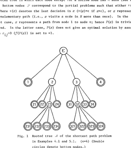
stands for the original problem.

be decomposed into n partial problems P(;rl),

P(x2), ... ,

P(xn).

f(P(x))

de-Each

P(x)

may Thus J3 (n) is a rooted tree in which each node except for a bottom node has n sons (see Fig. 1). Bottom nodes J correspond to the partial problems such that either 1T

(x)=

n,

where 1T(X) denotes the last decision in

x

(1T(X)=E if X=E), or

x

represents a nonelementary path (Le., x visits a node in N more than once). In the first case,

x

represents a path from node 1 to node n; hence

P(x)

is trivially solved. In the latter case,

P(x)

does not give an optimal solution by assump-tion c _ _ >0

(f(P(x))

is set to 00).

1-J

Fig. 1 Rooted tree J3 of the shortest path problem in Examples 4_1 and 5.1.

(n=4)

(Double circles denote bottom nodes.)

For this branching structure (J3 (n), 0, 1), (5: , g) may be defined as follows.

(4.5)

g(P(x) )=

100

if P(X)E Jand x represents a nonelementary path,

l cl' +C. .

+ ...

+c. . for x=ili? ... i

_{k ,}

otherwise.

~l ~1~2 ~k-l~k

-It is not difficult to see that these::; ,

g

satisfy all the conditions given in Section 2. Thus these give rise to a branch-and-bound algorithm A=«~(n),

0,

n,

(9,

g), s) for the shortest path problem.

To analyze the behavior of A, consider a special graph structure: N is the n'-stage graph with the start node in stage 0, m nodes in each of the stages 1, 2, ... , n'-l, and the terminal node in stage n~ N has n=mn~m+2 nodes. An arc exists from each node in stage i to any node in stage i+l, for i=O, 1,

... , n'-l. The length of each arc is determined as a random number taken

in-dependently from the same probability density function

q(x)

defined over [1,00).

q(x)

can be arbitrary as far as the useal assumptions to guarantee the central

limit theorem are satisfied. In particular, its mean exists and is denoted a

(~l). Since each arc has length not smaller than 1, the length of the

short-est path in this graph is at least

n'.

It is now easy to see that each partial problem, which is not a bottom node, has exactly m sons with finite g-values (of course, only nodes with

fi-n

'J

nite g-values can lead to a shortest path). Thus exactly

mla

partial prob-. n'

lems with finite g-values exist in depth L

a

~ of the branching structure. Let

I(n)=I'(n) denote the set of their indices. Then g(P_i ) of Pi' iEI(n), is the length of a path consisting of

~'

arcs (i.e., the sum of lengths of

l~'J

arcs). By the central limit theorem, therefore,

_,

g(P.) is normally

distrib-~

uted around its mean al~

1

(sn') if n' is sufficiently large. Thus the

proba-La

bility that g(P_i ) is not greater than the length of the shortest path (?n') is at least E=1/2 (>0).

Consequently the above model satisfies all the assumptions of Theorem 4.1 and hence T(n) grows at least as fast as exponentially with n' (i.e., n). Thus a branch-and-bound approach with lower bounding function (4.5) only is not competitive with other existing algorithms (e.g., [6]) which can obtain the shortest paths in polynomial time. By incorporating a dominance relation, however, the above branch-and-bound algorithm can be improved to a polynimial time algorithm, as shown in the subsequent sections.

Example 4.2.

Consider the flow-shop scheduling problem with n jobs and m machines [3]. Each job j (lsjsn) is processed on machines 1, 2, ... , m in this order. The processing time of job j on machine i is Pji (?O). \fuen only

per-Branch-and-Bound Algorithms 27

mutation schedules are permitted (i.e., all machines process jobs in the same order), find an optimal schedule (Le., an order of n jobs on machines) which minimizes the maximum completion time (makespan) on machine

m.

An obvious branching scheme for this problem is to decompose a partial problem in depth

k

(~n), given a subschedule for initial

k

jobs, into

(n-k)

partial problems by fixing the (k+l)st jab from the remaining

(n-k)

jobs. In this scheme, a partial problem in depth

k

is decomposed into

n-k

sons. The resulting branching structure is similar to Fig. I (except that no job appears more than once in a subschedule defining a partial problem). All partial problems in depth

n-l

belong to J" since the n-th job is then automatically determined. Fc;>r partial problem

P,

let

J(P)

denote the set of fixed jobs,

and

t .(P)

denote the completion time of job j

(EJ(P»

on machine

m

when jobs

J

in

J(P)

are processed in the order specified by

P.

It is then obvious that

(4.6)

satisfies all the conditions of a lower bounding function given in Section 2. The resulting branch-and-bound algorithnl

A,

however, satisfies all the assump-tions of Theorem 4.1 in certain cases as given below, and its T(~) must have an exponential growth.

Now assume that processing times

Poi

are independently determined from a

u

probability density function

q(x)

which is defined over [0, 00) and has mean

a

(~O). The minimum of the maximum completion time on machine m,

t

m, obviously satisfies

By the central limit theorem, again, t is normally distributed around its mean

a(n-IJ(P)

I)

if

n

is sufficiently large. Next, for partial problems

P

with

n

depth

m+l

(its index set is denoted

I(n)=I'(n»,

it is obvious that m

U(P)~

L L

p--(=t')

i=l jEJ(P)

J1.-n holds, and

t'

is also normally distributed around its mean

maIJ(P) I=ma

by

m+l

the central limit theorem. Since (1)

mean(t)=a(n-IJ(P) I)=a(n-

n

)~amn ~ma ~ =mean(t')

"1+1

m+l

m+l

holds for

IJ(p)

1= m~l

'

and (2)

t

and

t'

are independent random variables, the probability of g(P)S~ is at least E=1/2. Consequently, in this case, all the assumptions of Theorem 4.1 are satisfied.

func-tion (4.6) would not be efficient enough to solve large problems. When m is restricted to 2, however, a powerful method is known to improve its efficiency. It will be discussed as Example 6.2.

5.

Dominance Test

As mentioned in Section 1, the dominance test, which may be regarded as a generalization of the lower bound test, is sometimes incorporated in A3 (Test) of a branch-and-bound algorithm. It is based on a

dominance relation

t

D

which is a

partial ordering

on ~D satisfying

(i)

PjDP

_k

AP_j

f P

_k

imply

_f(Pj

> <

f(P

k

) ,

(ii)

PjDP

k

APj fPk

imply that for each descendant

P

k

,

of

P

k

,

there

ex-ists a descendant

P.,

of

P.

such that

P.,DP

k,.

J J J

By condition (i), we conclude that P

k does not provide an optimal solution of

Po

if

_Pj

satisfying

PjDP

_k

has already been generated. As a result, A3 may be modified as follows.

Modified A3

(Test)tt: Go to AS if

P

i

E9,

and go to A6 if

g(Pi»z

holds

or P

.DP.

holds for some P.

(fp.)

E JV. Otherwise go to A4. (JV denotes the set

J '& ~ J

of nodes currently generated, i.e., those which are active, terminated or de-composed.)

A branch-and-bound algorithm with this modified A3 is denoted A=«~,

0,

f),

(9,

g), D, s).

A primal motivation of introducing a dominance relation is to improve the computational efficiency by terminating a larger number of partial problems. This point will be further discussed in the next section. It is also inter-esting, however, to see that almost all algorithms of combinatorial optimiza-tion problems based on dynamic programming can be viewed as branch-and-bound using a dominance relation. (This point was first noticed by Kohler [20] and

t This definition is for the case in which all optimal solutions of

Po

is sought. For the case of seeking a single optimal solution, it should be slightly modified [15] but the following argument also holds true without any essential change.

tt

P.

is said

terminated

in A3 i f one of the conditions

P.E

9,

g(P.)

>z and

'& '& '&

P.DP.

holds.

Branch-and-Bound Algorithms 29

the dynamic programming approach to the traveling salesman problem [12] was formulated as a branch-and-bound algorithm using a dominance relation. Morin and Marsten [26], on the other hand, attempt to improve the dynamic programm-ing computation by usprogramm-ing a method based on the lower bound test of branch-and-bound algorithms.) A dominance relation thus adds another dimension of flex-ibility both in designing efficient braneh-and-bound algorithms and in unify-ing a wide variety of algorithms under the name of branch-and-bound.

As such. an example, we consider here the well known Dijkstra algorithm for the shortest path problem which apparently has never been considered as branch-and-bound. (For the description of the Dijkstra algorithm, see [5,6].)

Example 5!1.

Consider the branch-and-bound algorithm

A

discussed in Example 4.1 to obtain the shortest paths in a given complete graph with posi-tive arc lengths. In addition to the 10IVer bounding function g of (4.5), introduce a dominance relation

D

defined by

(5.1)

P (x) DP (y)

~

[

71

(x)

=71

(y)

and

g (P (x) ) <g (P (y) ) ] .

*

This

D

satisfies condition (i) since

g (P(x)) <g (P(x))

~ (\i' WE l: )

(g (P(m)) <g (P

(yw))) '9f(x)<f(y).

Condition (ii) is also satisfied since

P(x)DP(y)

~(\i'WE

*

l:

)(p(m)DP(yw)),

as is easily proved.

From these, we can now construct a branch-and-bound algorithm A=«~(n),

0, f),

Cc;:· ,

g), D, Sg)'

where

Sg

is the best-bound search function mentioned

in Section 2. A begins with decomposing

peEl

into

P(l), P(2), ... , Pen).

Dur-ing computation, only a partial problem

P(x)

satisfying

(5.2)

g(P(x))'Sg(P(y))

for a11

P(Y)E

JJ satisfying

7I(y)=7I(x)

can be decomposed, and the sequence of the decomposed partial problems P(;c l),

P(x

₂

),···, P(x

r

)

satisfies

by virtue of D and best-bound search. As a characteristic of best-bound search, the first partial problem

P(x)

tested in A3 satisfying

P(x)e

~ and

7I(x)=n

gives an optimal solution, and

z

is immediately set to

f(P(x))

(=the

length of the shortest path) from ro After then, no partial problem is

de-composed in A4 (since

z'Sg(P(x'))

for all the remaining partial problems

P(x')),

and A7 (Halt) is eventually reached_

It is now easy to see that A is essentially the same as the Dijkstra algorithm. (Although the Dijkstra algor:lthm is usually given in the form of obtaining a single optimal solution, the above algorithm obtai'ls all optimal

solutions. It can be easily modified to an algorithm for obtaining a single optimal solution.)

6. Upper Bound for T(A)

An upper bound for T(A) derivable from a dominance relation D is given in this section. This bound is sometimes useful to find a class of problems for which a branch-and-bound is particularly efficient, e.g., the shortest path problem of Example 5.1.

Let A=«....a, 0, f), (~;', g), D, sh) be a branch-and-bound algorithm with a heuristic search function (see Section 2). Heuristic search is adopted here since it includes most of the known search strategies, such as breadth-first search, depth-first search and best-bound search, as special cases [14). D is said consistent with h if P.DP. implies h(Pk)<h(P.) for any proper ancestor P_k

1- J J

of

P..

By definition of heuristic search, this implies that no proper ances-

1-tor of Pi is active when F'j is selected (Le., Pi has already been generated or a proper ancestor of Pi has been terminated). Next, D is consistent with g

i f P.DP. implies g(P.)<g(P.). (This notion was first introduced in [21).)

1- J 1- J

The above two types of consistency assumptions are in fact satisfied by many dominance relations proposed in the literature. For example, the domi-nance relation used in [16, 22) for the two-machine flow-shop scheduling prob-lem to minimize mean flow time (instead of makespan), and the one used in [29] for the one-machine scheduling problem with deadlines are consistent with g

and

h,

where heuristic search function sh in these algorithms represents breadth-first search.

Lemma 6.1.

D is consistent with a heuristic function h in each of the following cases.

(a)t h(Pk)<h(Pn ) i f Pn is a son of Pk,and P.DP.I\P.I-P. implies h(P.)<h(P.).

iC iC 1 - J 1 - J 1- J

(b) h=g (i.e., best-bound search) and

D

is consistent with g.

(c) sh is a breadth-first search function, and D satisfies that P.DP. 1- J

can hold only if P. and p. are in the same depth.

1- J

Now recall that D is a partial ordering on p P.E J> is minimal with J

respect to D if no P.I-P.E ~D satisfies P.DP.. The set of minimal nodes is

de-1-J 1-,7

noted byp D'

Branch-and-Boumi Algorithms 31

Lemma 6.2. For a branch-and-bound a.lgorithm A= «...E, 0, f),

(9.

g), D,

sh)'

assume that

D

is consistent with both

g

and

h.

Then any

PjE

JD decomposed

in

A

is minimal with respect to

D.

Proof: Assume that

P.DP.

and

P.jP..

Since

D

is consistent with

h, 1).

'l.-J 'l.-J

'I.-has already been generated (Le.,

PiE

JI') or ancestor

P

k

of

Pi

has been

termi-nated when

P

_j is selected. In the first case,

P

_j is terminated in A3 by the dominance test. Thus consider the second case; three cases are possible.

(a)

_Pk

has been terminated in A3 by

PkE

9.

Then

_{z(Pj )$z(Pk )$f(Pk )5f(Pi )}

since

P.

is selected after

P

_k

'

where

z(P,.)

is the incumbent value when

P.

is

J d J

selected. Furthermore note that

f(Pi)=g(P

_i

)

(since

PiE

9

by condition CC) of

9)<g(Pj )

(sinse

D

is consistent with

g)

holds. Thus

P

_j

is terminated in A3

by

_{g(Pj»z(Pj ).}

(b)

P

_k

has been terminated in A3 by

g(Pk»z(P

_k

).

Then

g(P

_k

)5g(P

_i

)

(by condition (c) of

g)<g(P.)

(since

D

is consistent with

g),

and z(Pk)~z(P.)

J J

since

P.

is selected after

P

_k• Thus

g(P .)'>z(P.)

and

P.

is also terminated.

J ~. J J

(c)

_Pk

has been terminated in A3 by

PaDP

_k

for some

PaE

JI'. Then some descendant

Pa'

of

P

_a

satisfies

Pa,DP

_i

by condition (ii) of a dominance rela-tion, and

P ,TJP.AP.DP.

implies

P ,DP.

since

D

is a partial ordering (hence

a ' l . - ' l . - J a J

transitive). Now assume that

P ,

is eventually generated in

A.

It is then a

generated before

P

_j by the consistency assumption with respect to

h.

Thus

P

_j

is also terminated in A3. Finally consider the case in which a proper ances-tor

P

b

of

P ,

a has been terminated (and

F ,

a was not generated). We may then

apply the same argument as above to

P

_b

instead of

Pa'.

This process, however, cannot continue indefinitely since ~~ is finite. Consequently, it is proved that P. is also terminated.

0

J

Theorem 6.3. Let A=«...E, 0, f), (:;:, g), D, Sh) be a branch-and-bound

algorithm with D consistent with both g and h. Then T(A) 51p - :;:

I.

D

Proof: Immediate from Lemma 6.2.

0

The lower bound of T(A) obtained in Theorem 3.1 for a branch-and-bound algorithm without using the dominance test can also be generalized to the case using it.

Theorem 6.4. Let A=«...E, 0, f), U;, g), D, s) be a branch-and-bound

algorithm (s may be any search function and D may be any dominance relation). Then T(A)~I(J - C; )npDI.

Proof: It was shown in the proof oE Theorem 3.1 that no

PiE

J - c,,' can

be terminated in A3 by

PiE

S. or

g(P

_i

) >zU)i).

In addition, no

PiEJ) D

can be terminated by

P .DP.

for some P.E cif since

Po.

is minimal with respect to

D.

0

Example 6.1.

Consider the shortest path problem of Examples 4.1 and 5.1. By definition of D (see (5.1», i t is obvious that D is consistent with g. D

is also consistent with h by Lemma 6.1 (b), since the algorithm of Example 5.1 uses best-bound search. From (4.5) and (5.1), it is also obvious that P(x) is minimal with respec t to D i f and only i f g (P (x» <:g (P (y» for any y wi th TT (y)

=

TT(X). Therefore, under assumption (2.2) (i.e., no two partial paths have the

same length), there is exactly one minimal partial problem for each node i in the given network N. Thus 1'))D1=n, and the P(x) in P

D with TT (x)=n satisfies P(X)EC;. This shows that I fl

D- C, I=n-l and T(A)~n-l by Theorem 6.3. (If some

partial paths have the same length, this number increases correspondingly, since all shortest paths are to be sought.)

Example 6.2.

Consider the flow-shop scheduling problem introduced in Example 4.2. For this problem, no powerful dominance relation is known at present. Moreover, it is known that the flow-shop scheduling problem with m?3

is NP-complete [7, 24], thereby suggesting that there exists no dominance re-lation D such that it can be tested in polynomial time whether P.DP. holds for

& J

a given pair p. and P., and T(A) of the resulting branch-and-bound algorithm A

1. ,7

is bounded by a polynomial (since otherwise A is an algorithm to solve an NP-complete problem in polynomial time, that is most unlikely).

For the flow-shop scheduling problem with m=2, however, there is a clas-sical polynomial time algorithm due to Johnson [18] (see also [3]). We do not give a detailed description of the Johnson algorithm, but point out that it can be viewed as a branch-and-bound algorithm with the following dominance re-lation

D.

(6.1) PkDP£ = ( a ) IJ(P_k) 1=IJ(P£)i (Le., P_k and P£ are in the same depth), (b) there exists exactly on et pair of jobs j l and j2 such that j l is forced to be processed before j2

in PI< but j2 is forced to be processed before j l in P£,

and (c) min[P

J" ₁ I' PJ' ₂ 2]<min[P. _{J 2} I' p. _{J l} 2]'

Note that j l is forced to be processed before j2 in P if either (1) j l ' j2E

J(P) and j l is fixed to be processed before j2' or (2) jlEJ(P) and j2'J(P).

The proof that D of (6.1) is in fact a dominance relation is omitted since i t is essentially the same as Johnson's proof [18].

Now i t is not difficult to show that exactly one partial problem in each

Hranch·and·Bound A 19ori thm.~ 33

depth of the branching structure belongs to J)D i f min [P. l' P. 2 J=min [P. l'

J_l J₂ J₂

To apply Theorem 6.3, consider a P. 21 does not hold for any pair

J

l and

J

2. J l

branch-and-bound algorithm with breadth-first search function (then Lemma 6.1 (c) holds). The resulting algorithm satisfies T(n)<;IJ!D- C;1=n-L Finally i t

is straightforward to show that this braneh-and-bound algorithm is equivalent to Johnson's original algorithm in the sense that the same sequence of partial problems are tested in both algorithms.

Acknowledgements

The author wishes to thank Professors H. Mine and T. Hasegawa of Kyoto University for their support and comments. He is also indebted to Miss T. Kanazawa for her excellent typing.

References

L Agin, N.: Optimum Seeking with Branch and Bound. Managenent Science, Vol. 13 (1966), pp. B176-B185.

2. Bellmore, B. and Nemhauser, G.L.: The Traveling Salesman Problem: A Survey. Operations ReseaY'ch, VoL 16 (1968), pp. 538-558.

3. Conway, R.W.: Maxwell, W.L., and Miller, L.W.: Theory of Scheduling, Addison-Wesley, Reading Mass., 1967.

4. Cook, S.A.: The Complexity of Theorem Proving Procedures. Proc. 3Y'd ACM Conference on Theory of Computing, (191'0), pp. l5l-lSH.

5. Dijkstra, E.W.: A Note on two Problems in Connexion with Graphs. Numerische Mathematik, vol. 1 (1959), pp. 269-271.

6. Dreyfus, S.E.: An Appraisal of Some Shortest Path Algorithms. Operations ReseaY'ch, vol. 17 (1969), pp. 394-411.

7. Garey, M.R., Johnson D.S., and Sethi, R.: The Complexity of Flowshop and Jobshop Scheduling. Technical Report No. 168, The Pennsylvania State Uni-versity, Computer Science Department, 1975.

8. Geoffrion. A.H .• and Harsten, R.E.: Integer Programming Algorithms:

A Framework and State-of-the-Art Survey. Managpment SC1:ence, voL 18 (1972). pp. 469-49L

9. Girfinkel, R.S., and Nemhauser, G.L.: Tntegep Programming, John Wiley and sons, New York, (1972).

10. Golomb, S.W., and Baumert, L.D.: Backtrack Programming. JouY'rIal of the A CM, vol. 12 (1965), pp. 516-524.

11. Hart, P.E., Nilsson, N.J., and Raphael, B.: A Formal Basis for the heuris-tic Determination of Minimal Cost Paths. IEEE TY'ansact1:ons on System sci-ence and CybeY'netics_, Vol. SSC-4 (1968), pp. 100-107.

12. Held, M., and Karp, R.M.: A Dynamic Programming Approach to Sequencing Problems. JouY'nal of SIAM, vol. 10 (1962), pp. 196-210.

13. Held, M., and Karp, R.M.: The Traveling Salesman Problem and Minimum Span-ning Trees: Part 2. Mathematieal PY'ogY'amming, vol. 1 (1971), pp. 6-25. 14. Ibaraki, T.: Theoretical Comparisons of Search Strategies in Branch-and-Bound Algorithms. Inter>national Jour>nal of ComputeY' and Infor>mation sci-ences, Vol. 5 (1976), pp. 315-344.

15. Ibaraki, T.: The Power of Dominance Relations in Branch-and-Bound Algo-rithms. Working Paper, Dept. of Applied Mathematics and Physics, Kyoto University, 1975; to appear in JOUY'nal of the ACM.

16. Ignall, E., and Schrage, L.E.: Application of the Branch and Bound Tech-nique to Some Flow-Shop Sequencing Problems. OpeY'ations ReseaY'ch, Vol. 13

(1965), pp. 400-412.

17. Jeroslow, R.G.: Trivial Integer Programs Unsolvable by Branch-and-Bound. Mathematical PY'ogY'amming, Vol. 6 (1974), pp. 105-109.

18. Johnson, S.M.: Optimal Two- and Three-stage Production Schedules with Setup Times Included. Naval ReseaY'ch Logistics QuaY'teY'ly, Vol. 1 (1954). 19. Karp, R.M.: Reducibility among Combinatorial Problems. In Complexity of

ComputeY' Computation."!, Miller, R.E., and Thatcher, J.W. (eds.), Plenum Press, New York, 1972, pp. 85-103.

20. Kohler, W.H.: Exact and Approximate Algorithms for Permutation Problems. Ph. D. Disseration, Princeton University, 1972.

21. Kohler, W.H., and Steiglitz, K.: Characterization and Theoretical Compari-son of Branch-and-Bound Algorithms for Permutation Problems. Jour>nal of the ACM, Vol. 21 (1974), 140-156.

22. Kohler, W.H., and Steiglitz, K.: Exact, Approximate, and Guaranteed Accu-racy Algorithms for the Flow-Shop Problem n/2/F/F. JouY'nal of the ACM, Vol. 22 (1975), pp. 106-114.

23. Lawler, E.L., and Wood, D.E.: Branch-and-Bound Method: A Survey. 0pcY'-ations ReseaY'ch, Vol. 14 (1966), pp. 699-719.

24. Lenstra, J.K., Rinooy Kan, A.H.G., and Brucker, P.: Complexity of Machine Scheduling Problems. Ann. DiscY'ete Mathematics, Vol. 1, to appear.

Branch·and·Bound A igorithms 35

25. Mitten, L.G.: Branch-and-Bound Method: General Formulation and Properties. Operations Research, Vol. 18 (1970), pp. 24-34.

26. Morin, T.L., and Marsten, R.E.: Branch-and-bound Strategies for Dynamie Programming. Operations Research~ Vo1 .. 24 (1976), pp. 611-627.

27. Ni1sson, N.J.: Problem-Solving Methods in Artificial Intelligence, McGraw-Hill, New York, 1971.

28. Poh1, I.: First Results on the Effect of Error in Heuristic Search. In Machine Intelligence 5, Me1tzer, B., and Michie, D. (eds.), Edinburgh University Press, 1969.

29. Sahni, S.K.: Algorithms for Scheduling Independent Tasks. Journal of the A CM, Vol. 23 (1976), pp. 116-127.

Toshihide IBARAKl: Department of Applied Mathematics and Physics, Faculty of Engineering, Kyoto University, Kyoto 606, Japan.