Time Dependence Structures of Hedge Fund Index Returns: Regime Switching Volatility and Crisis State 利用統計を見る

Time Dependence Structures of Hedge Fund Index

Returns: Regime Switching Volatility and

Crisis State

著者

Midori Munechika

journal or

publication title

The Economic Review of Toyo University

volume

46

number

2

page range

121-145

year

2021-03-10

Time Dependence Structures of Hedge Fund Index Returns:

Regime Switching Volatility and Crisis State

Midori Munechika

Abstract

This study considers the time series of four primary strategies of hedge fund index returns over the period of April 1, 2003 to March 16, 2017. In particular, we examine the specific characteristics of each strategy in left tail events by using the Markov regime switching model and allowing for possible regime shifts that affect both the means and variances. This study adopts the two-step estimation procedure. First, we identify time dependence structures of the four hedge fund index returns by the autoregressive moving average-generalized autoregressive conditional heteroscedasticity (ARMA-GARCH) modeling to detect the conditional heavy tails of standardized residual distributions. Second, we employ the Markov regime switching methodology to model the volatility of the left-tail events in each strategy. The results suggest that volatility persistence of hedge fund returns stems from not only long memory, but also structural breaks. In particular, we observe that structural breaks had a strong impact on their volatility persistence during the financial crisis of 2007-2009. Key words: ARMA-GARCH, regime switching volatility, long memory, structural shift

Contents 1. Introduction

2. Hedge Fund Index Returns  2.1. Stylized Facts

 2.2. Data Descriptions

3. Identifying Time Dependence Structures  3.1. Absence of Autocorrelations  3.2. ARMA-GARCH Modeling

 3.3. ARMA-GARCH Estimates 4. Markov Regime Switching Model  4.1. Mixtures of Normal Distributions

 _{4.2. Regime Switching Model allowing Switching Mean and Volatility}  4.3. Selection of the Number of Regimes

 4.4. Three State Model and Crisis State 5. Concluding Remarks

1. Introduction

We know that the risk-return characteristics of hedge fund strategies differ significantly from traditional investment strategies as well as among individual hedge fund strategies. Prior studies such as Brooks and Kat [2002], and Edwards and Gaon [2003], have examined the unique statistical properties of hedge fund index returns since the early 2000s. The objective of analyzing the data-generating process of hedge fund index returns is to understand the underlying phenomena that gave rise to the origination of this data consisting of various dynamics of the strategies, such as leverage, short selling, and derivatives, and switching investment positions with the evolving market conditions.

Detection of time dependency in financial time series is a crucial issue for financial modeling since time dependency in asset returns may occur at several levels. Jondeau, Poon and Rockinger [2007] point out two important aspects. First, statistical tests using unconditional statistics and the inferences derived thereof could be misleading in the case of time dependent return distribution. Second, the full exploitation of time dependency will help to produce better forecasts, thereby contributing toward risk management and asset allocation.

It is paramount importance to construct a parsimonious model that adequately explains the data-generating process for examining the risk-return profile of hedge funds and revealing the underlying phenomena. This is because contradictory results arise from differences in methodologies, time periods, and data frequencies. The purpose of constructing the statistical models discussed in this study is to gain a better understanding of hedge fund return volatility, especially for left-tail events. The ultimate aim of volatility analysis is to identify the cause of volatility.

This study proceeds as follows. Section 2 presents the data descriptions and stylized facts of asset returns as the cornerstone of the argument for revealing unique characteristics of hedge fund index returns. Section 3 identifies time dependence structures of four hedge fund index returns by using the ARMA-GARCH specifications and the remaining issues on adequatly modeling return volatility. Section 4 introduces the Markov regime switching model to capture the volatility behavior of hedge fund index returns during left-tail events. We

find that three states provide the optimal number of regimes and that describes the volatility behavior during the financial crisis of 2007-2009. Section 5 provides summary and concluding remarks on the study.

2. Hedge Fund Index Returns

2.1. Stylized Facts

Many empirical studies report a set of common statistical properties across a wide range of asset returns known as stylized facts. Theoretical models such as the mean-variance analysis rest on the basis of the standard assumption of normality for asset return distributions. The statistical properties identified as stylized facts invalidate many of the conventional models used to study financial time series.

It is important to consider the statistical features of hedge fund indices based on stylized facts as an intermediate step between the description of data-generating process and the modeling of hedge fund indices. Cont [2001] conducted a thorough survey on stylized facts, such as distributional properties, tail properties, and extreme fluctuations, and examined the statistical problems encountered in financial modeling. The main stylized facts closely related to this study are as follows.

1. Heavy tails: The unconditional distribution of asset returns has a heavier tail than a normal distribution. 2. Asymmetry: The unconditional distribution of asset returns exhibits skewness that depicts the asymmetry

of the distribution.

3. Aggregational Gaussianity (normality): As the time span of the returns increases, the return distribution becomes closer to the normal distribution. In particular, the shape of the distribution is not the same at different time scale.

4. Absence of autocorrelations: Asset returns generally do not exhibit significant autocorrelations except for very small intraday time scales.

5. Volatility clustering: The amplitude of asset returns varies over time. Volatility of returns is positively autocorrelated suggesting that the magnitude of the change is sometimes large and sometimes small, which tend to cluster with time. Volatility clustering can be captured by the positive autocorrelation coefficients of squared returns.

6. Volatility asymmetry: Most of the measures of volatility of an asset are negatively correlated with the returns of that asset, resulting in a leverage effect.

7. Conditional heavy tails: Even after correcting for volatility clustered returns by applying GARCH-type models, the residual time series still exhibit heavy-tails that are less heavy than in the unconditional distribution of asset returns.

stylized facts from 4 to 6 are related to time dependency in returns and volatility. 2.2. Data Descriptions

In this study, we analyze four principal hedge fund indices obtained from the HFRX Single Strategy Indices of the Hedge Fund Research, Inc. database. The data were collected daily from March 31, 2003 to March 16, 2017. The HFRX Single Strategy Indices correspond to the HFRX Equity Hedge Index, the HFRX Event Driven Index, the HFRX Macro/CTA Index, and the HFRX Relative Value Arbitrage Index. These four single strategy indices constitute the HFRX Global Hedge Fund Index which is designed to be representative of the overall composition of the hedge fund universe.1）

First, Equity Hedge is a directional and equity-based strategy maintaining long and short positions primarily in equity and equity derivative securities. The aim is not to be market neutral. Its investment decision includes both quantitative and fundamental techniques, broadly diversified strategies or narrowly focused on specific sectors, and frequently employed leverage. Second, Event Driven strategy focuses specifically on corporations involved in special situations or significant restructuring events such as mergers, liquidations and insolvencies. The aim of this strategy is to take advantage of price anomalies triggered by special events. Securities vary according to their order of repayment in the capital structure from senior to junior or subordinated securities that frequently involve additional derivative securities. Event Driven strategy is categorized as a non-directional and mispricing strategy. Third, Macro/CTA is a directional strategy, based on the prediction to future macroeconomic movements, whose managers employ a variety of techniques. Fourth, Relative Value Arbitrage is an arbitrage strategy that takes advantage of temporary mispricing valuations in the relationship between multiple securities. It involves a broad range across equity, fixed income, derivative, or other types of security and is a non-directional strategy.

Different sampling frequencies of time series data may display different properties even though they originate from the same data-generating process. In particular, the shape of the distribution is not the same at different time scales. For example, the statistical distributions of hedge fund indices are different from changes in daily returns to changes in monthly returns. Therefore, we report both monthly and daily returns of the four hedge fund indices, whose summary statistics are shown in Table 1. Returns are computed as the first difference of the logarithm of the hedge fund index values. Let Pt be the hedge fund index value at time t,

such that the hedge fund index return rt is defined as:

   rt=ln(Pt / Pt-1)＊

100

=(pt −pt-1)＊

100

(

1

)   

where pt=ln(Pt) is the logarithm of the hedge fund index value measured in percentage over the period of t-

1

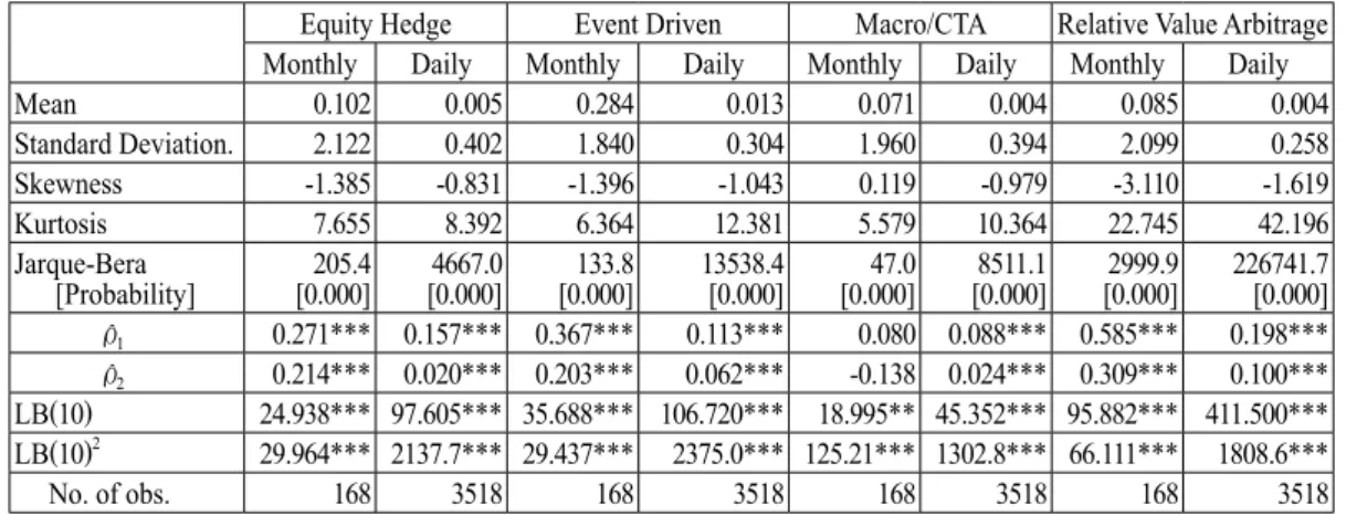
to t.2）

The summary statistics suggest the following. First, there are considerable differences in the risk and return characteristics among the four hedge fund investment strategies. For monthly and daily returns, Event Driven and Macro/CTA have the highest and lowest means, respectively. Standard deviation is a commonly used metric for volatility. While Equity Hedge has the highest standard deviation for monthly and daily returns, Event Driven and Relative Value Arbitrage have the lowest standard deviation for monthly and daily returns, respectively.

Second, skewness depicts asymmetry of the distribution (stylized fact 2). Four index return distributions indicate negative skewness, except for the monthly return distribution of Macro/CTA. When skewness is negative, large negative returns are more likely to appear than large positive returns. Such a distribution indicates that the negative tail, that is the tail on the left-hand side, is longer than the positive tail. The left-tail is particularly extreme.

Third, kurtosis captures the thickness of the distribution s tail relative to a normal distribution (stylized fact 1). Positive kurtosis exceeding that of a normal distribution, which has a kurtosis of three, is said to be leptokurtic. This property is the sign of a heavy-tailed distribution with the highest peak. All indices exhibit leptokurtic distributions. In particular, the distributions of daily returns are more heavy-tailed that of monthly returns since kurtosis increases from monthly returns to daily returns. A heavy-tailed distribution is more prone to extreme values, which are known as outliers. In this case, we observe occasional extreme changes in returns. Clark [1973] documents that the return is leptokurtic as its interval reduces and the number of observations increases. It can be

2）  Log return rt is also known as the continuous compounded return. A key advantage of using the log return is its

ag-gregation property, that is, multiple period return is simply the sum of single period log returns. Table 1：Summary Statistics of Hedge Fund Index Returns

Equity Hedge Event Driven Macro/CTA Relative Value Arbitrage Monthly Daily Monthly Daily Monthly Daily Monthly Daily

Mean 0.102 0.005 0.284 0.013 0.071 0.004 0.085 0.004 Standard Deviation. 2.122 0.402 1.840 0.304 1.960 0.394 2.099 0.258 Skewness -1.385 -0.831 -1.396 -1.043 0.119 -0.979 -3.110 -1.619 Kurtosis 7.655 8.392 6.364 12.381 5.579 10.364 22.745 42.196 Jarque-Bera   [Probability] [0.000]205.4 [0.000]4667.0 [0.000]133.8 13538.4[0.000] [0.000]47.0 [0.000]8511.1 [0.000]2999.9 226741.7[0.000]    ρ₁ 0.271*** 0.157*** 0.367*** 0.113*** 0.080 0.088*** 0.585*** 0.198***    ρ₂ 0.214*** 0.020*** 0.203*** 0.062*** -0.138 0.024*** 0.309*** 0.100*** LB(10) 24.938*** 97.605*** 35.688*** 106.720*** 18.995** 45.352*** 95.882*** 411.500*** LB(10)2 _{29.964*** 2137.7*** 29.437*** 2375.0*** 125.21*** 1302.8*** 66.111*** 1808.6***} No. of obs. 168 3518 168 3518 168 3518 168 3518

Note: The sample period varies from April 2003 to March 2017 for monthly returns and from April 1, 2003 to March 16, 2017 for daily returns.

seem from the comparison between the monthly and daily returns that due to Aggregational Gaussianity (stylized fact 3), the return distribution approaches the normal distribution as the time span of the returns increases. Thus, the daily return distributions tend to generate more outliers than monthly return distributions.

Fourth, the normality test based on the Jarque-Bera statistic suggests that unconditional return distributions of hedge fund indices are highly non-normal. This non-normality strongly focuses attention on two statistical phenomena. First, extreme events occur more often than predicted by a normal distribution, corresponding to excess kurtosis. Leptokurtosis implies high occurrence of outliers, that have a powerful effect on the variance, that is, volatility. Volatility clustering exhibits these events to be clustered. Second, crises occur more often than booms, which are reflected in negative skewness. Therefore, if we use the standard normal assumption to apply financial modeling, we will fail to evaluate the number and magnitude of crises and booms. The negatively skewed and heavy-tailed distributions relate hedge fund index returns to outlier-prone probability distributions. Therefore, outliers should be examined closely because extreme events are quite different from those occurring under normal market conditions and may have new information about tail risk events.

Fifth, for time dependency in returns, the estimated first and second order autocorrelation coefficients and the Ljung-Box Q statistic (LB) up to the tenth order in levels and squares of returns confirm sufficient evidence on the existence of serial correlation. The first order autocorrelations ρ1 for monthly returns are high for Relative

Value Arbitrage (0.585) and Event Driven (0.367), while that of Equity Hedge (0.271) and Macro/CTA (0.080) are moderate, and low, respectively. Billio, Getmansky, Lo and Pelizzon [2010] state that hedge fund indices are divided into liquid and illiquid strategies corresponding to indices with first-order autocorrelations (ρ1) for return

less than and equal to or greater than 0.30, respectively. According to this indicator, Equity hedge and Macro/ CTA are characterized as liquid strategies, while Event Driven and Relative Value Arbitrage are categorized as illiquid strategies. Our results are consistent with Getmansky, Lo, and Makarov [2004] who argue that serial correlation primarily occurs due to illiquidity exposure and smoothed returns. Event Driven and Relative Value Arbitrage involving illiquid assets tend to have higher values of autocorrelated coefficients, while Equity Hedge and Macro/CTA involving liquid assets tend to have lower values. The estimated daily autocorrelations are much lower than the monthly strategy indices. Moreover, the LB joint test statistic up to the tenth order in levels of returns (LB(10)) rejects the null hypothesis of no autocorrelation for lags 1 to 10 in the hedge fund index returns at the 1% level of statistical significance for all the cases except for the monthly return of Macro/CTA where the null hypothesis is rejected at the 5% level of significance. The results suggest that the absence of autocorrelations (stylized fact 4) is rejected. Significant positive autocorrelation means performance persistence.

Sixth, time dependency in volatility can be examined in the same approach as the test for returns. A common measure of volatility clustering is the autocorrelation function to the squared returns.

Non-zero autocorrelation in squared returns is evidence of volatility time dependence. In Table 1, LB(10)2

shows the Ljung-Box statistic up to the tenth order in squares of returns. The results indicate that squared returns strongly exhibit positive autocorrelations reflecting the phenomenon of volatility clustering, that is, persistence of volatility. Volatility behavior is often referred to as heteroscedasticity. Time varying volatility is also referred to as stochastic volatility. This implies that there is a memory effect in financial time series data. Volatility clustering (stylize fact 5) is strongly confirmed by the hedge fund index returns.

3. Identifying Time Dependence Structures

3.1. Absence of Autocorrelations

The term random walk (RW) originates from the fact that all future price changes represent random departure from the past prices, and thus, cannot be predicted. The RW model is a benchmark in financial modeling, especially for speculative prices that are expressed in their logarithmic forms. It is often associated with the idea of the efficient market hypothesis (EMH). According to the EMH, equity market is extremely efficient in reflecting all information about stocks. It is well known that price movements in liquid markets such as equity markets do not exhibit any significant autocorrelation (stylized fact 4). The simple RW model can be stated as:

   pt = pt−1+εt (2)   

where pt = ln(Pt) and εt is the white noise, εt ~i.i.d. N(

0

,σ2). We express return as the difference of the series,

   rt=pt−pt-1=εt (3)   

where εt is not serially uncorrelated. Consequently, according to the RW model, equation (3) states that the

returns exhibit the absence of autocorrelation, which is the theoretical bases of stylized fact 4.

In order to test whether the time series is a RW process or not, we consider the first-order autoregressive (AR) model:

   pt=Øpt-1+εt (4)   

We want to test Ø=1 since random walks are AR(1) processes with unit roots. The ordinary least squares (OLS) estimates Ø＾ is often very close to 1. However, we have to know whether Ø=0.99 implies that the price is predictable such that market timing is possible, whereas Ø=1 (i.e. random walk) implies it is not. The basic objective of the unit root test in time series is to examine the null hypothesis, H0: Ø=1 in equation (4) against

the one-sided alternative hypothesis, H1: Ø<1. Therefore, the hypotheses of interest are H0: the series contains

a unit root against H1. When the null hypothesis is rejected the series is stationary.

 We conducted the Phillips-Perron (PP) test for unit root on the hedge fund index returns, which is similar to the augumented Dickey-Fuller (ADF) test, but allow for autocorrelated residuals. In addition to the PP test, we conducted confirmatory data analysis with the joint use of stationarity test, that is, the

Kwiatkowski-Phillips-Schmidt-Shin (KPSS) test.3） _{Unit root tests confirm that the time series of four hedge fund index}

values in logarithmic forms are not rejected to the null hypothesis, that is, the RW process. However, the return series (the first difference of the index values in logarithmic forms) are rejected, that is, the stationary time series.4）

Time dependency in asset returns may occur at several levels: serial correlation in returns, volatility and volatility asymmetry. We know that hedge fund returns exhibit a strong positive serial correlation. Table 1 suggests that the absence of autocorrelations in returns (stylized fact 4) is denied for all hedge fund indices based on the Ljung-Box Q statistic. Significant positive autocorrelation means performance persistence. However, volatility clustering (stylized fact 5) is strongly confirmed by the hedge fund index returns.

3.2. ARMA-GARCH Modeling

Statistical properties of the hedge fund index returns examined in Section 2.2 exhibit autocorrelated and volatility clustered returns. Time series with autocorrelation behavior in returns and volatility are often modeled by autoregressive moving average (ARMA) process and autoregressive conditional heteroskedasticity (ARCH) process, respectively. This section briefly introduces the recent study, Munechika [2015] to fit the ARMA-GARCH model in our historical return data.

The ARMA model is a popular method for modeling stationary time series. The idea behind autoregressive (AR) process is to feed past return into the current return since a time series variable often relates to its past values in many cases. The AR(p) model is formulated as

   rt= Ø1rt-1 +Ø2rt-2+…+Øprt-p+εt=∑pi=1 Øi rt-p +εt, t=1,..., n (5)   

Here, Ø1, ..., Øp are the values of the parameters that measure the impact of the previous return and lie

between -1 to +1.

In general, the return on any asset rt can be divided into two parts: the expected part of the return E[rt] and

the unexpected part of the return εt.

   rt = E [rt] +εt (6)   

   r t =μ+εt (7)   

where μ denotes the mean (i.e., the expected value of the return). One problem with AR models is that they often require a large value of p to fit the data. A solution to this problem is to add a moving average (MA) component to an AR(p) process. The process rt is a MA process if it can be expressed as a weighted average

3） For more details, see Brooks [2014], p.365.

(moving average) of the past values of the white noise (εt). The MA process formulates the structure of the

error term. The MA(q) process can be written as

   r t = μ+εt+θ1εt-1 +θ2εt-2+…+θqεt-q=μ+∑qj=1θjεt-q (8)   

where θ1, …, θq scales the influence of the white noise process. The general ARMA (p, q)model is obtained

by combining the AR(p) and MA(q) processes.

   rt =μ+∑pi=1 Øi r t-p +εt +∑qj=1 θjεt-q (9)   

In many cases, an ARMA process provides a parsimonious parameterization.

Engle [1982] initially modeled volatility clustering, measured by serially correlated squared returns, with the ARCH model. The ARCH(p) model assumes that the conditional variance is a linear function (i.e., a moving average) of the past p squared innovations:

   ht =σt2 =ω+α1ε2t-1+…+αpε2t-p =ω+ ∑pi=1 αiε2t-1 (10)   

where σt2 is a conditional variance, ω is a constant term, and αp is a reaction coefficient.

The ARCH(p) model can be regarded as an AR(p) model for the squared innovation εt2, that cares for the time

dependency in volatilities. The ARCH model often requires a large p to fit the data-generating process because of the large persistence in volatility. Bollerslev [1986] proposed more parsimonious GARCH model that captures long-lagged effects with fewer parameters. The conditional variance of a GARCH(p, q) model is defined as:    ht =σt2=ω+∑pi=1αiε2_t-11+∑qj=1βjσ2t-j (11)   

where βq is a persistent coefficient. The parameters must satisfy the constraints: ω> 0, αp≥ 0 and βq ≥ 0. The

condition αp+βq<1 ensures stationarity. The GARCH model is formed by augmenting the AR components

in the ARCH model with components that are similar to the MA model. The ARCH and GARCH models are useful in describing time-varying conditional variance, which partially explains the heavy-tailed phenomenon present in returns. Bollerslev and Wooldridge [1992] state that in most applications p = q is sufficient due to the increase in log-likelihood of the GARCH(1,1) model over the class of GARCH(p, q) models.

Although the GARCH models can capture volatility clustering as well as some degree of heavy-tailedness, they cannot take account of an asymmetric effect on the conditional variance. The GJR model (Glosten, Jagnnathan, and Runkle [1993]) are often applied to examine an asymmetric impact of volatility to shocks (stylized fact 6).5）

We estimated three types of GARCH models consisting of two equations: the equations for conditional mean and conditional variance. The equation for conditional mean is specified by the ARMA process, as

5） The exponential GARCH (EGARCH) model (Nelson [1991]) also captures the leverage effect. We estimated both models and found that the GJR model was preferred as the fitted model by the selection criteria (Schwarz information criterion and Akaike information criterion, and the Log-likelihood), as shown in Table 2.

shown in equation (9).

First, the conditional variance equation of GARCH(1,1) model is described as

   σ_t2=ω+α1ε2t-1 +β1σ2t-1 (12)   

where σt2 is the conditional variance, ω is the constant term, α1 is a reaction coefficient and β1 is a persistent

coefficient. The parameters must satisfy the constraints: ω> 0, α1 ≥ 0 and β1 ≥ 0.

 Second, the conditional variance equation of GJR(1,1) model is

   ht =σt2=ω+α1ε2t-1 +γdt-1ε2t-1 +β1 ht-1 (13)        dt= 1 εt< 0 (bad news)      0 εt≥ 0 (good news) (14)     where γ is known as the asymmetry or leverage term. When γ=0, the GJR model converges to the standard GARCH form. However, when the shock is positive (i.e., good news) the effect on volatility is α1 but when

the shock is negative (i.e., bad news) the effect on volatility is α1+γ. Threfore, as long as γ is significant

and positive, negative shocks have a larger effect on volatility than positive shocks. 3.3. ARMA-GARCH Estimates

Here, the ARMA-GARCH specifications are conducted by using the daily return data from April 1, 2003 to March 16, 2017. The ARMA-GARCH models are estimated in a two-step procedure. In the first step, the parameters of the ARMA models for rt are estimated based on the Box-Jenkins approach, which takes three

steps: identification, estimation, and diagnostic checking. The selected ARMA process for the conditional mean equations based on the Schwarz information (SIC) criterion are AR(1) process for Equity Hedge and Macro/CTA and ARMA(2,1) process for Event Driven and Relative Value Arbitrage.

In the second step, let the residuals of the ARMA models be denoted by εt . The parameters of the GARCH

(1,1) models are estimated.

   ε_t =σt vt (15)   

To allow for the possibility of nonnormality in the conditional distribution of returns, we assume that the vt

is independently identically distributed (i.i.d.) from the Student t distributed errors for the GARCH and GJR models and the generalized error distribution (GED) for the exponential GARCH (EGARCH) model.6）

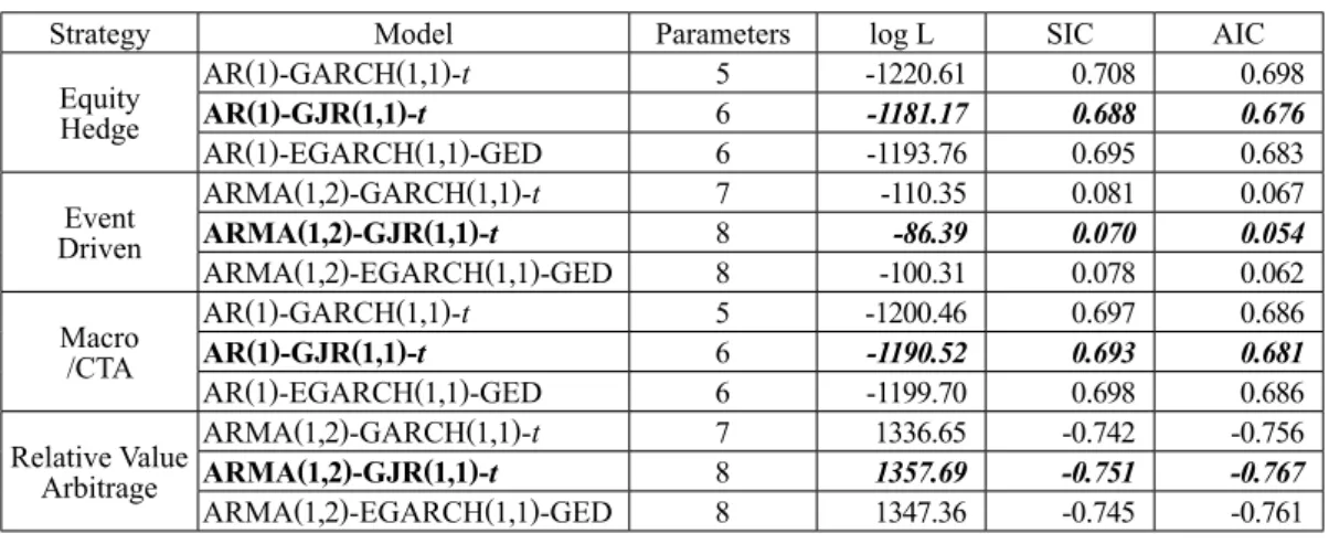
Table 2 reports the model selection statistics. Our investigation finds that based on the values of information criteria, such as the SIC and Akaike information criterion (AIC), and the log-likelihood,

ARMA-6） The use of Student t distribution instead of a normal one is popular in the GARCH literature. See Bollerslev, Chou and Kroner [1992].

GJR(1,1) modeling with Student t distributed error is the best model. Therefore, we present the estimated results of the ARMA-GARCH(1,1) and the ARMA-GJR(1,1) models here.

The estimation results of the ARMA-GARCH specifications are summarized in Table 3. First, for the conditional mean equations, the estimated ARMA process for Event Driven and Relative Value Arbitrage exhibit statistically significant and large positive values of coefficients for the AR(1) terms and large negative values of coefficients for the MA(1) terms. These estimates indicate that the return to the nondirectional strategies (Event Driven and Relative Value Arbitrage) have high serial correlation. The most likely explanation is that the indices to these hedge fund strategies involve less liquid assets. On the contrary, the directional strategies such as Equity Hedge and Macro/CTA exhibit relatively low serial correlation.

Second, for the conditional variance equations, the results indicate that the volatility of hedge fund index returns is quite persistent since the sum of α＾₁ and β＾₁ is close to unity. The half-life period (HLP) of volatility (in Table 3) takes 19.01 days for Equity Hedge, 37.95 days for Event Driven, 38.16 days for Macro/CTA, and 53.80 days for Relative Value Arbitrage, respectively.7） _{Therefore, the volatility of all hedge fund index}

returns demonstrates long memories.

Third, volatility asymmetry is examined through the estimation of the ARMA-GJR models. The coefficient α

＾₁ implies an impact of good news, while the sum of α＾_1＋γ＾ implies an impact of bad news. The estimated values of the coefficient γ＾ are positive for Equity Hedge, Event Driven, and Relative Value Arbitrage, which confirm the leverage effect for three index returns. However, only Macro/CTA indicates that the coefficient γ＾

7） The half-life period (HLP) is the length until half of the volatility, which is computed as HLP=log(0.5)/log(α＾1＋β＾1）.

See Füss, Kaiser and Adames [2006].

Table 2：Comparison of Selection Information for the ARMA-GARCH models

Strategy Model Parameters log L SIC AIC

Equity Hedge AR(1)-GARCH(1,1)-t 5 -1220.61 0.708 0.698 AR(1)-GJR(1,1)-t 6 -1181.17 0.688 0.676 AR(1)-EGARCH(1,1)-GED 6 -1193.76 0.695 0.683 Event Driven ARMA(1,2)-GARCH(1,1)-t 7 -110.35 0.081 0.067 ARMA(1,2)-GJR(1,1)-t 8 -86.39 0.070 0.054 ARMA(1,2)-EGARCH(1,1)-GED 8 -100.31 0.078 0.062 Macro /CTA AR(1)-GARCH(1,1)-t 5 -1200.46 0.697 0.686 AR(1)-GJR(1,1)-t 6 -1190.52 0.693 0.681 AR(1)-EGARCH(1,1)-GED 6 -1199.70 0.698 0.686 Relative Value Arbitrage ARMA(1,2)-GARCH(1,1)-t 7 1336.65 -0.742 -0.756 ARMA(1,2)-GJR(1,1)-t 8 1357.69 -0.751 -0.767 ARMA(1,2)-EGARCH(1,1)-GED 8 1347.36 -0.745 -0.761

is negative, which implies an inverse leverage (negative asymmetric) effect.

Finally, the standardized residuals of these models still exhibit the heavy-tailed distributions, whose tails are lighter than that in the unconditional distributions of hedge fund index return shown in Table 1. This is because the series of returns contains some isolated outliers that cannot be effectively modeled by the GJR model.

If the selected model is the true model, the standardized residuals are i.i.d. N (0.1). One way of testing Table 3 : ARMA-GARCH and GJR Modeling

ARMA-GARCH(1,1) modeling ARMA-GJR(1,1) modeling Equity

Hedge DrivenEvent Macro/CTA

Relative Value Arbitrage

Equity

Hedge DrivenEvent Macro/CTA

Relative Value Arbitrage AR(1) ARMA(1,2) AR(1) ARMA(1,2) AR(1) ARMA(1,2) AR(1) ARMA(1,2) Conditional Mean equation

μ＾ 0.0353*** _0.0386*** _{-0.0077 0.0206}*** _0.0243*** _0.0308*** _{0.0108 0.0162}** (0.0061) (0.0065) (0.0053) (0.0043) (0.0061) (0.0073) (0.0053) (0.0052) Ø ＾₁ 0.1596*** _0.9646*** _0.0443*** _0.9552*** _0.1626*** _0.9676*** _{0.0397 0.9657}*** (0.0181) (0.149) (0.0172) (0.0141) (0.0177) (0.0117) (0.0167) (0.0090) θ＾₁ ― -0.8623*** _{― -0.8614}*** _{― -0.8664}*** _-0.8707*** (0.0238) (0.0224) (0.0214) (0.0193) θ＾₂ ― -0.0766*** _{― -0.0525}*** _{― -0.0708}*** _-0.0512*** (0.0184) (0.0177) (0.0179) (0.0172)

Conditional Variance equation

ω＾ _0.0055*** _0.0016*** _0.0029*** _0.0007*** _0.0075*** _0.0019*** _0.0018*** _0.0007*** (0.0011) (0.0004) (0.0007) (0.0001) (0.0011) (0.0003) (0.0005) (0.0001) α＾1 0.1253*** 0.0984*** 0.0873*** 0.0939*** 0.0067 0.0141 0.1011*** 0.0371*** (0.0147) (0.0120) (0.0112) (0.0112) (0.0133) (0.0125) (0.0149) (0.0101) γ＾ ― ― ― ― 0.1953*** _0.1185*** _-0.0634*** _0.1129*** (0.0247) (0.0176) (0.0148) (0.0180) α＾1＋γ＾ ― ― ― ― 0.2020 0.1326 0.0377 0.1500 β＾₁ 0.8389*** _0.8835*** _0.8947*** _0.8932*** _0.8331*** _0.8964*** _0.9222*** _0.8909*** (0.0176) (0.0132) (0.0125) (0.0108) (0.0167) (0.0119) (0.0104) (0.0106) α＾₁＋β＾₁ 0.9642 0.9819 0.9820 0.9872 HLP 19.01 37.95 38.16 53.80 SIC 0.7080 0.0813 0.6966 -0.7415 0.6879 0.0700 0.6933 -0.7512 LogL -1220.61 -110.35 -1200.46 1336.65 -1181.17 -86.395 -1190.52 1357.688 Standardized Residuals: z＾t=ε＾t /σ＾t Mean -0.0649 -0.0537 -0.0078 -0.0317 -0.0379 -0.0342 -0.0180 -0.0146 Standard Deviation 0.9999 0.9996 1.0030 0.9863 1.0042 1.0025 1.0024 0.9923 Skewness -0.5187 -0.4702 -0.5032 -0.1343 -0. 5149 -0.5087 -0.4678 0.0582 Kurtosis 5.0037 5.0747 6.3747 6.0297 5.3912 5.117 5.8820 6. 7105 Jarque-Bera 746.10*** _760.364***_1817.307***_1355.673*** _993.264*** _934.806***_1345.462***_2019.503***

Notes: Based on daily continuously compounded returns for 3517 observations from April 1, 2003 to March 16, 2017; standard errors are presented in parenthesis; ***, **, * denote the statistical significance at 99%, 95%, and 90% confidence levels, respectively.

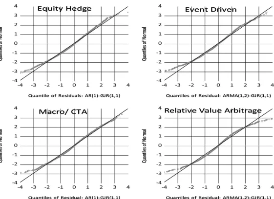
the distribution of the residuals is with the help of quantiles. Figure 1 displays the quantile-quantile (QQ) plots of the standard residuals of the ARMA-GJR modeling against a normal distribution for the four index returns. The data is plotted with quantile residuals on the horizontal axis and theoretical quantiles on the vertical axis. All the QQ-plots are convex-concave curves, implying that they possess heavier tails than the normal distribution. These plots indicate that these models cannot capture large negative shocks that deviate from normality, since GARCH-type models assume that the tails of this distribution reflect the same dynamic behavior in the rest of the distribution. These observations have motivated us to model the left-tail of the distribution of hedge fund index returns.

4. Markov Regime Switching Model

Markov regime switching models can provide a systematic method for modeling structural breaks and regime shifts in the hedge fund index return data-generating process. Long memory has been defined in terms of decay rates of long-lag autocorrelations resulting from time dependency. ARMA and GARCH models corresponding to the level of returns and variance, respectively, specify long memory. However, volatility

Figure 1：Standardized Residuals of the ARMA-GJR (1,1) Estimates Against QQ Plot of the Normal Distribution

-4 -3 -2 -1 0 1 2 3 4 -4 -3 -2 -1 0 1 2 3 4

Quantile of Residuals: AR(1)-GJR(1,1)

Qu an tiles of No rm al Equity Hedge

Quantile of Residuals: AR(1)-GJR(1,1)

Qu an tiles of No rm al Equity Hedge -4 -3 -2 -1 0 1 2 3 4 -4 -3 -2 -1 0 1 2 3 4

Quantiles of Residual: ARMA(1,2)-GJR(1,1)

Qu an tiles of No rm al Event Driven

Quantiles of Residual: ARMA(1,2)-GJR(1,1)

Qu an tiles of No rm al Event Driven -4 -3 -2 -1 0 1 2 3 4 -4 -3 -2 -1 0 1 2 3 4

Quantiles of Residual: AR(1)-GJR(1,1)

Qu an tiles of No rm al Macro/ CTA

Quantiles of Residual: AR(1)-GJR(1,1)

Qu an tiles of No rm al Macro/ CTA -4 -3 -2 -1 0 1 2 3 4 -4 -3 -2 -1 0 1 2 3 4

Quantiles of Residual: ARMA(1,2)-GJR(1,1)

Qu an tiles of No rm al

Relative Value Arbitrage

Quantiles of Residual: ARMA(1,2)-GJR(1,1)

Qu an tiles of Nor ma l

persistence may originate from structural changes in the variance process in addition to long memory. For instance, if there are the periods during which variance is high but constant for some time and low but constant in other times, persistence of such high and low volatility periods results in volatility persistence. GARCH models cannot capture persistence of such periods.

4.1. Mixtures of Normal Distributions

The Markov regime switching models are latent variable time series models and represent a special class of dependent mixtures of several processes, in which an unobservable m-state Markov process determines the state or regime and a state-dependent process of observations. The Markov process can be described as an i.i.d. mixture distributions. When the process is in regime 1, the observed return rt is presumed to have been drawn

from a given normal distribution, denoted by N(μ1, σ21). If the process in regime 2, then rt is drawn from a

N (μ2, σ22) distribution, and so on. The parameter μ is a location parameter and σ is a scale parameter. A

mixture of two normal distributions with equal means and different variances is called a scale mixture, and a mixture distribution with different means and equal variances is called a location mixture. A location mixture yields a negatively skewed distribution and a scale mixture results in heavier tails. Hence, mixtures of normal distributions can produce a skewed and heavy-tailed distribution (stylized facts 1 and 2).8）

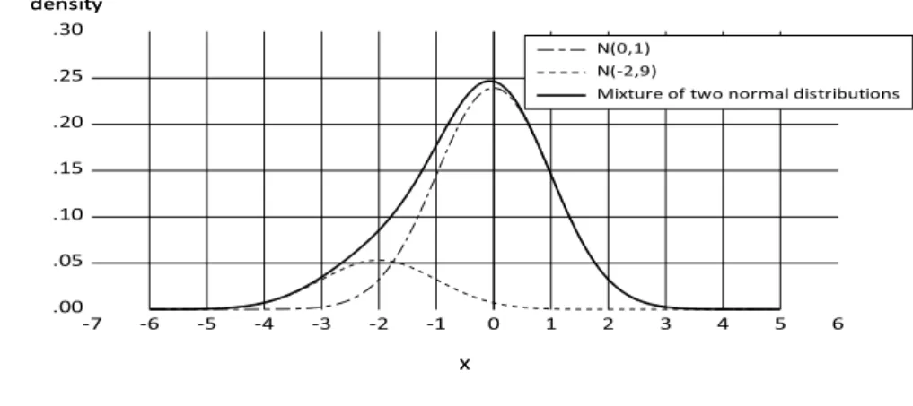
Consider two location mixtures of two normal distributions, with rt |st=1~N(0, 1) and rt |st=2~N(-2, 9), where

the probability of obtaining state 1 is P{st=1}=0.6 and state 2 is P{st=2}=0.4. Figure 2 shows the mixture

distribution comprising two regimes. The idea behind the regime switching approach is based on the unconditional probability distribution for the observed variable rt that can be produced by a mixture of two Gaussian variables,

8） See Hamilton [1994] and Gentle [2020] in more detail about mixtures of distributions. Figure 2：Mixture of Normal Distributions

.00 .05 .10 .15 .20 .25 .30 -7 -6 -5 -4 -3 -2 -1 0 1 2 3 4 5 6 X N(0,1) N(-2,9)

Mixture of two normal distributions

density

X

allowing the skew or kurtosis to be different from that of a single Gaussian variable. The mixture distribution shown in Figure 2 is negatively skewed and heavy-tailed. Ruppert [2004] states that normal mixture distribution is more prone to outliers than a normal distribution with the same mean and standard deviation. Thus, large negative returns should be much more concerned about if the return distribution is similar to a normal mixture distribution rather than a normal distribution. In the context of hedge fund return volatility, a Markov process can be used to govern the switches between regimes with different variances.

4.2. Regime Switching Model allowing Switching Mean and Volatility With a regime switching approach, equation (7) can be written as:

   rt =μt (st ) +εt (st), (16)   

where μt (st ) is a switching mean, εt (st) is a switching variance, and both functions of st {j=1,2,…, N}

indicate the regime at time t. Equation (16) can be written as:

   rt =μt (st ) +σt (st) zt , (17)   

where zt is i.i.d.~N (0.1) from standard normal distributed errors. At time t, the actual process generating

the data is determined by the realization of the unobservable discrete variable st, which is known as a state

variable or regime. This model allows for a change from the presence of discontinuous shifts in mean and volatility of returns in response to occasional short-lived events. The change in regime is itself an unobservable random variable. Therefore, the model includes a description of the probability law governing the change from state to state.

A Markov chain can be used to govern the switches between regimes where the unobserved variable st

is characterized by state dynamics following a first-order Markov process. It assumes the probability that st

being equal to some particular value j depends on the past through the most recent value st-1 :

   Pr{st=j | st-1=i, st-2=k, ... }=Pr{st=j | st-1=i}=pij. (18)   

The dynamics behind the switching process is driven by a transition matrix that collects the transition probabilities in an (N×N） matrix P :

      p11 … p1N

   P =

[

⋮    ⋮

]

(19)   

      pN1 … pNN

The transition probabilities of the Markov chain link each state in the chain to the next. The transition matrix P denotes the probabilities of moving regimes. For example, the element p21 (in row 2, column 1) gives the

probability of state transition from state 2 to state 1 in the next period. Note that

   pi1 + pi2 + … + piN = 1. (20)   

central points of the structure of a Markov regime switching model. 4.3. Selection of the Number of Regimes

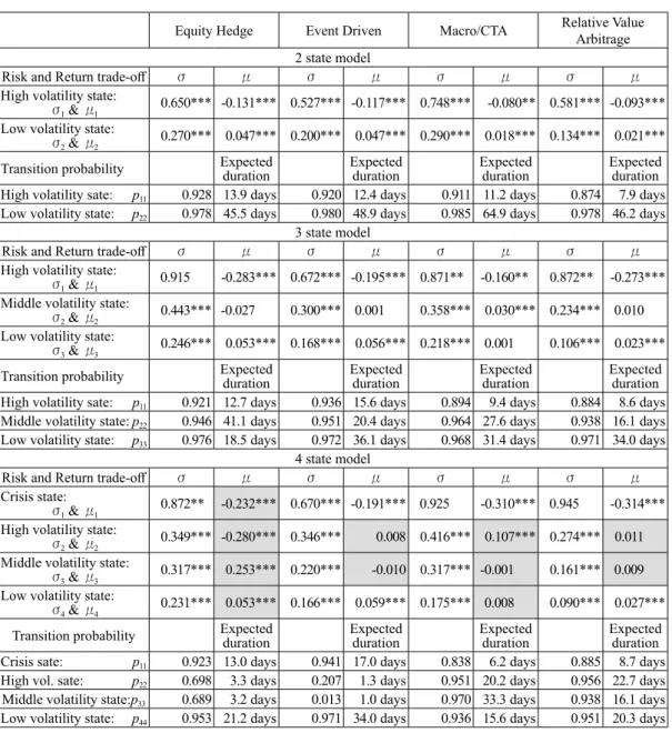
To determine the number of regimes used in the estimation, we estimate and examine the Markov regime switching model with up to four regimes. Table 4 reports the maximum-likelihood estimates of the mean and standard deviations, as well as the transition probabilities of staying in the same state with each expected duration. We primarily discuss the choice of the optimal number of regimes based on the results obtained to capture the left-tail risk behavior of the hedge fund returns.

We focus on the volatility of the model and label the states as, high and low with respect to the value of the volatility for the two-state specification. A low volatility state with high mean and high volatility state with low mean are referred to as the conventional taxonomy of bull and bear markets. The three-state specification corresponds to high, middle and low volatility states, while the four-state specification corresponds to crisis, high, middle and low volatility states, respectively.

Several authors such as Wang and Theobald [2008] stressed that the selection of the regime switching process is difficult because the identification cannot be observed through the simple use of statistical tests such as likelihood ratio, Lagrange multiplier, or Wald tests. Moreover, in practical applications, it is not easy to distinguish persistent level shift from a single outlier, especially for daily data set.

Table 5 reports the model selection statistics based on the information criteria and log-likelihood estimates following Hamilton and Susmel [1994]. The optimal model is selected following the minimum information criteria (AIC, SIC, and Hannan-Quinn) and maximum log-likelihood statistics. All statistics select the four-regime specification. However, there are some difficulties in its practical application.

First, the most serious problem lies in the two-step procedures of estimation. The estimation procedures of the four state model contain an additional step that uses the restricted matrix on transition probabilities after the estimation based on the unrestricted matrix. The two and three state specifications are conducted by using the unrestricted matrix on transition probabilities only. Following Hamilton and Susmel [1994], we initially conduct the maximum likelihood estimates with no constraints on any of the transition probabilities

pij under the conditions 0≤ pij≤1 and ∑4i=1 pij＝1. In the four state specification, a number of unrestricted

estimates in the transition probability matrix fell on the boundary pij＝0. Consequently, they did not converge

for the calculation of standard errors, which is a possible explanation for the difficulty in model specification. Therefore, to re-estimate the model, we impose the restriction pij＝0 on transitions to calculate the standard

errors, such that these parameters are treated as known constants.

from the two and three state specifications (Table 4). The mean value is approximately the same and tends to zero in the daily return data set. In the four state specification, our results show that the mean is approximately the same in the crisis and high volatility states for Equity Hedge, high and middle volatility states for Event Driven and Relative Value Arbitrage, and middle and low volatility states for Macro/CTA. Consequently, the four state specifications for all hedge fund indices exhibit an inverse relationship of risk-return trade-off

Table 4：Estimation Results of Regime Switching Model

Equity Hedge Event Driven Macro/CTA Relative Value _Arbitrage

2 state model

Risk and Return trade-off σ μ σ μ σ μ σ μ

High volatility state:

σ1 & μ1 0.650*** -0.131*** 0.527*** -0.117*** 0.748*** -0.080** 0.581*** -0.093*** Low volatility state:

σ_{2 & μ2} 0.270*** 0.047*** 0.200*** 0.047*** 0.290*** 0.018*** 0.134*** 0.021***

Transition probability Expected _duration Expected _duration Expected _duration Expected _duration

High volatility sate: p11 0.928 13.9 days 0.920 12.4 days 0.911 11.2 days 0.874 7.9 days

Low volatility state: p22 0.978 45.5 days 0.980 48.9 days 0.985 64.9 days 0.978 46.2 days

3 state model

Risk and Return trade-off σ μ σ μ σ μ σ μ

High volatility state:

σ1 & μ1 0.915 -0.283*** 0.672*** -0.195*** 0.871** -0.160** 0.872** -0.273*** Middle volatility state:

σ2 & μ2 0.443*** -0.027 0.300*** 0.001 0.358*** 0.030*** 0.234*** 0.010 Low volatility state:

σ_{3 & μ3} 0.246*** 0.053*** 0.168*** 0.056*** 0.218*** 0.001 0.106*** 0.023***

Transition probability Expected _duration Expected _duration Expected _duration Expected _duration

High volatility sate: p11 0.921 12.7 days 0.936 15.6 days 0.894 9.4 days 0.884 8.6 days

Middle volatility state: p22 0.946 41.1 days 0.951 20.4 days 0.964 27.6 days 0.938 16.1 days

Low volatility state: p33 0.976 18.5 days 0.972 36.1 days 0.968 31.4 days 0.971 34.0 days

4 state model

Risk and Return trade-off σ μ σ μ σ μ σ μ

Crisis state:

σ1 & μ1 0.872** -0.232*** 0.670*** -0.191*** 0.925 -0.310*** 0.945 -0.314*** High volatility state:

σ2 & μ2 0.349*** -0.280*** 0.346*** 0.008 0.416*** 0.107*** 0.274*** 0.011 Middle volatility state:

σ_{3 & μ3} 0.317*** 0.253*** 0.220*** -0.010 0.317*** -0.001 0.161*** 0.009 Low volatility state:

σ4 & μ4 0.231*** 0.053*** 0.166*** 0.059*** 0.175*** 0.008 0.090*** 0.027***

Transition probability Expected _duration Expected _duration Expected _duration Expected _duration

Crisis sate: p11 0.923 13.0 days 0.941 17.0 days 0.838 6.2 days 0.885 8.7 days

High vol. sate: p22 0.698 3.3 days 0.207 1.3 days 0.951 20.2 days 0.956 22.7 days

Middle volatility state:p33 0.689 3.2 days 0.013 1.0 days 0.970 33.3 days 0.938 16.1 days

Low volatility state: p44 0.953 21.2 days 0.971 34.0 days 0.936 15.6 days 0.951 20.3 days

Table 5：Summary Statistics for Model Selection

Index _RegimeNo. of _parametersNo. of AIC SIC Hannan-_{Quinn likelihood}

Log-Equity Hedge 2 6 0.754 0.764 0.757 -1319.5 3 9 0.720 0.741 0.728 -1255.2 4 12 0.697 0.721 0.706 -1211.6 Event Driven 2 6 0.137 0.148 0.141 -235.5 3 9 0.092 0.113 0.100 -150.3 4 12 0.088 0.113 0.097 -141.4 Macro/CTA 2 6 0.739 0.750 0.743 -1294.4 3 9 0.705 0.726 0.713 -1228.4 4 12 0.689 0.716 0.699 -1197.4 Relative Value Arbitrage 2₃ 6₉ -0.594_-0.699 -0.583_-0.678 -0.590_-0.691 1050.4_1241.1 4 12 -0.723 -0.699 -0.715 1286.3

Figure 3：Distribution of States

Low 79.7% Low 51.7% 49.5%Low High 20.3% Middle 40.0% Middle _18.8% High 8.3% High 23.4% Crisis 8.3% 0% 20% 40% 60% 80% 100% 2 R E G I M E 3 R E G I M E

E

Eqquuiittyy H

4 R E G I M E

Heeddggee

Low 76.4% Low 59.3% Low 55.0% High 23.6% Middle 34.6% _{Middle 18.4%} High 6.1% High 18.9% Crisis 7.6% 0% 20% 40% 60% 80% 100% 2 R E G I M E 3 R E G I M E 4 R E G I M E Low 85.2% Low 35.4% Low 19.2% High 14.8% Middle 56.1% Middle 55.0% High 8.4% _High 19.8% Crisis 6.0% 0% 20% 40% 60% 80% 100% 2 R E G I M E 3 R E G I M E 4 R E G I M E Low 85.3% Low 58.6% _Low 36.9% High 14.7% Middle 36.7% Middle 37.7% High 4.7% High 21.7% Crisis 3.7% 0% 20% 40% 60% 80% 100% 2 R E G I M E 3 R E G I M E 4 R E G I M E

R

Reellaattiivvee V

Vaalluuee A

Arrbbiittrraaggee

E

Eqquuiittyy H

Heeddggee

E

Evveenntt D

Drriivveenn

M

across states, which should be considered as a misspecification.

Third, according to distribution of states in each regime (Figure 3), the state probabilities of the high volatility of the three state and crisis states of the four state specifications, are not changing and are approximately the same in individual strategies. The distribution of states in the middle volatility state of the three state model is essentially divided into the high and middle volatility states of the four state model.

The principle of parsimony indicates that for more complex models (i.e., the use of more parameters) to hold, the fit of the models should be significant. As per the problems discussed above, the three state model with regime dependent volatility and mean is the most parsimonious model that captures the tails of the distribution. In this study, we found a significant improvement in fit for the hedge fund index returns after adding the third regime to the second regime. However, there was no significant improvement in fit after the inclusion of the fourth regime. The use of three regimes is optimal for our analysis

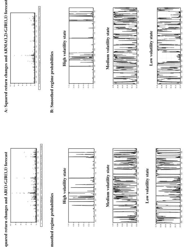
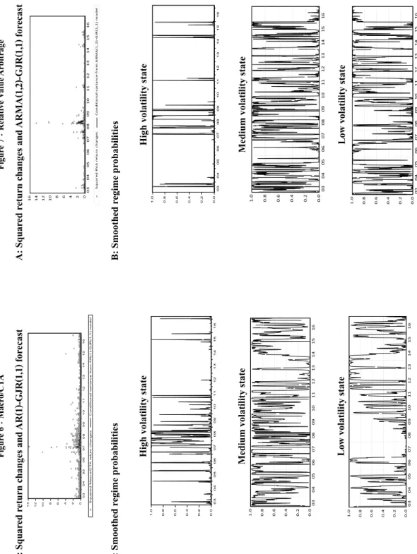
4.4. Three State Model and Crisis State

Figures 4-7 provide an additional insight into the three state regime switching model. Panel A of Figure 4, 5, 6 and 7 gives an indication of the volatility clustering (i.e., squared return changes) and the estimated forecasts of conditional variance based on the individual preferred ARMA-GJR models of four hedge fund index returns. All four plots show substantial volatility clustering. This is confirmed by the reported Ljung-Box statistic for squared returns, as these are significant at the 1 % level (Table 1). The plots also demonstrate that the ARMA-GJR specifications cannot fully capture the persistence of shocks in volatile periods. This is confirmed by the reported standardized residuals of the ARMA-GJR (1,1) estimates against the QQ plot of the normal distribution (Figure 1). A shock can be followed by a volatile period not only because of ARCH effects, but also because of the switch to a high volatility regime.

Panel B of Figure 4, 5, 6 and 7 plots the estimated smoothed regime probabilities of the three states.9） _The

smoothed probabilities provide insights into the timing of each volatility state. With regard to the evolution of the high volatility state, Macro/CTA has experienced a more frequent regime shifts than other strategies. Sudden shifts in the variance are more important for the interpretation of Macro/CTA than for other strategies. Although there is a certain degree of variability in the evolution of the high volatility state among the four strategies, the high volatility states in Panel B are in synchronization with the time period that exhibits a

9） The smoothed regime probability is constructed by using the entire sample of observations. Klaassen [2001] discussed the two types of regime probabilities, ex ante and smoothed regime probabilities, and concluded that the smoothed re-gime probability provides the most informative answer to indicate the rere-gime in which the process was likely in at time t.

marked difference between squared return changes and the ARMA-GJR specifications in Panel A. It reveals that volatility persistence may originate from structural changes in the variance process, that is, such high volatility periods may persist. It is to be noted that the high volatility state increased during the years of 2007 and 2008 for all strategies. This period coincides with global financial crisis of 2007-2009.

Figur e 4 ： Equity Hedge A: Squar ed r

eturn changes and

AR (1 )-GJR (1,1 ) for ecast 0 2 4 6 8 10 03 04 05 06 07 08 09 10 11 12 13 14 15 16 Sq ua re dE Hr et ur nc ha n ges Co nd it io na lv ar ia nc ef ro mA R(1 )-G JR (1 ,1 )m ode l B: Smoothed r egime pr obabilit ies

High volatility state

0. 0 0. 2 0. 4 0. 6 0. 8 1. 0 03 04 05 06 07 08 09 10 11 12 13 14 15 16 Medium volatilit y state 0. 0 0. 2 0. 4 0. 6 0. 8 1. 0 03 04 05 06 07 08 09 10 11 12 13 14 15 16 Low volatilit y state 0. 0 0. 2 0. 4 0. 6 0. 8 1. 0 03 04 05 06 07 08 09 10 11 12 13 14 15 16 Figur e 5 ： Event Driven A: Squar ed r

eturn changes and

ARMA (1,2 )-GJR (1,1 ) for ecast 0 2 4 6 8 10 12 03 04 05 06 07 08 09 10 11 12 13 14 15 16 Sq ua re dE Dr et ur nc ha ng es Co nd it io na lv ar ia nc ef ro mA RM A( 1, 2 )-G JR (1 ,1 )m odel B: Smoothed r egime pr obabilit ies

High volatility state

0. 0 0. 2 0. 4 0. 6 0. 8 1. 0 03 04 05 06 07 08 09 10 11 12 13 14 15 16 Medium volatilit y state 0. 0 0. 2 0. 4 0. 6 0. 8 1. 0 03 04 05 06 07 08 09 10 11 12 13 14 15 16 Low volatilit y state 0. 0 0. 2 0. 4 0. 6 0. 8 1. 0 03 04 05 06 07 08 09 10 11 12 13 14 15 16

Figur e 7 ： Relative Value Arbitrage A: Squar ed r

eturn changes and

ARMA (1,2 )-GJR (1,1 ) for ecast 0 2 4 6 8 10 12 14 16 03 04 05 06 07 08 09 10 11 12 13 14 15 16 Sq ua re dR VA re tu rn change s Cond itio na lv ar ia nc ef ro mA RM A( 1,2) -G JR (1,1 )m od el B: Smoothed r egime pr obabilit ies High volatilit y state 0. 0 0. 2 0. 4 0. 6 0. 8 1. 0 03 04 05 06 07 08 09 10 11 12 13 14 15 16 Medium volatilit y state 0. 0 0. 2 0. 4 0. 6 0. 8 1. 0 03 04 05 06 07 08 09 10 11 12 13 14 15 16 Low volatilit y state 0. 0 0. 2 0. 4 0. 6 0. 8 1. 0 03 04 05 06 07 08 09 10 11 12 13 14 15 16 Figur e 6 ： Macr o/CT A A: Squar ed r

eturn changes and

AR (1 )-GJR (1,1 ) for ecast 0 2 4 6 8 10 12 14 03 04 05 06 07 08 09 10 11 12 13 14 15 16 S qu ar ed Ma cr o/ CT Ar et ur nc ha n ges Co nd it io na lv ar ia nc ef ro mA R(1 )-G JR (1 ,1 )m odel B: Smoothed r egime pr obabilit ies

High volatility state

0. 0 0. 2 0. 4 0. 6 0. 8 1. 0 03 04 05 06 07 08 09 10 11 12 13 14 15 16 Medium volatilit y state 0. 0 0. 2 0. 4 0. 6 0. 8 1. 0 03 04 05 06 07 08 09 10 11 12 13 14 15 16 Low volatilit y state 0. 0 0. 2 0. 4 0. 6 0. 8 1. 0 03 04 05 06 07 08 09 10 11 12 13 14 15 16

5. Concluding Remarks

This study investigates the volatility behavior of four primary hedge fund index returns, especially focusing on their tail behavior. First, the study uses the ARMA-GARCH-type model to examine time dependence structures of the four hedge fund index returns, that is, Equity Hedge, Event Driven, Macro/CTA, and Relative Value Arbitrage. The estimated results exhibit that volatility of returns in response to shock is highly persistent for all strategies, confirming volatility asymmetry, and leverage effect (except for Macro/ CTA). Leverage effect implies that a decrease in the value of hedge fund index may lead to a greater increase in volatility than in the case of an increase in the value of an index of the same magnitude. Only Macro/ CTA demonstrates an inverse asymmetric effect. Moreover, empirical estimates reveal that the fundamental innovations are much better described as coming from a Student t distribution than by a normal distribution.

Second, this study uses the Markov regime switching model, allowing three regimes to affect both mean and variance. The choice of a Markov regime switching model stems from the failure of the ARMA-GARCH model to detect the left-tail of the distribution of returns. The ARMA-GARCH-type model cannot particularly capture large negative shocks that are deviating from normality. The estimates suggest a strong evidence of switching behavior in hedge fund index returns. This was observed during the financial crisis of 2007-2009 when high volatility state captured extreme return behavior. Hence, the persistence of high volatility state yields an extra source of volatility persistence that explains substantial volatility clustering in the period of financial crisis. Marco/CTA has experienced more frequent regime shifts than other strategies. Moreover, sudden structural shifts in the variance are more important for the interpretation of Macro/CTA than other strategies.

【References】

Alexander, C. and Dimitriu, A. [2005], Detecting Switching Strategies in Equity Hedge Funds, ISMA Centre Discussion

Papers in Finance, DP2005-07.

Bauwens, L., Hafner, C. and Laurent, S. (eds.), [2012], Handbook of Volatility Models and Their Applications, John Wiley & Sons, Inc.

Billio, M., Getmansky, M. and Pelizzon, L. [2008], Crises and Hedge Fund Risk, Working Paper, No.10, 2008, Department of Eonomics Ca Foscari University of Venice.

Billio, M., Getmansky, M., Lo, A. W. and Pelizzon, L. [2010], Measuring Systemic Risk in the Finance and Insurance Sectors, MIT Sloan School Working Paper, 4774-10.

Blazsek, S. and Downarowicz, A. [2011], Forecasting Hedge Fund Volatility: A Markov Regime-Switching Approach,

Working Paper, available at SSRN:http://ssrn.com/abstract = 1768864.

Bollerslev, T. [1986], Generalized Autoregressive Conditional Heteroskedasticity , Journal of Econometrics, Vol. 31, pp. 307-327. Bollerslev, T., Chou, R. Y. and Kroner, K. F. [1992], ARCH Modeling in Finance: A Review of the Theory and Empirical

Evidence , Journal of Econometrics, Vol. 52, pp. 5-59.

Bollerslev, T. and Wooldridge, J. M. [1992], Quasi-maximum Likelihood Estimation and Inference in Dynamic Models with Time-Varying Covariances , Econometric Reviews, Vol. 11, No. 2, pp. 143-172.

Brooks, C. and Kat, H. M. [2002], The Statistical Properties of Hedge Fund Index Returns and Their Implications for Investors , The Journal of Alternative Investments, Vol. 5, No. 2, Fall, pp. 26-44.

Brooks, C. [2014], Introductory Econometrics for Finance, 3rd_{. ed., Cambridge University Press.}

Chan, N., Getmansky, M., Hass, S. M. and Lo, A. W. [2005], Systemic Risk and Hedge Funds, MIT Sloan Research Paper, No. 4535-05.

Chan, N., Getmansky, M., Hass, S. M. and Lo, A. W. [2006], Do Hedge Funds Increase Systemic Risk? Economic Review, Federal Reserve Bank of Atlanta, Fourth Quarter, pp. 49-80.

Christoffersen, P. F. [2012], Elements of Financial Risk Management, 2nd _{ed., Academic Press, Elsevier.}

Clark, P. K. [1973], A Subordinated Stochastic Process Model with Finite Variance for Speculative Prices , Econometrica, Vol. 41, No. 1, pp. 135-155.

Cont, R. [2001], Empirical Properties of Asset Returns: Stylized Facts and Statistical Issues , Quantitative Finance, Vol. 1, No. 2, pp. 223-236.

Del Brio, E. B., Mora-Valencia A. and Perote, J. [2014], Semi-Nonparametric VaR Forecasts for Hedge Funds During the Recent Crisis , Physica A, Vol. 401, pp. 330-343.

Diebold, F. X. and Inoue, A. [2001], Long Memory and Regime Switching, Journal of Econometrics, Vol. 105, No. 1, pp. 131-159.

Edwards, F. R. and Gaon, S. [2003], Hedge Funds: What Do We Know? , Journal of Applied Corporate Finance, Vol. 15, No. 4, pp. 58-71.

Engle, R. F. [1982], Autoregressive Conditional Heteroscedasticity with Estimates of the Variance of United Kingdom Inflation , Econometrica, Vol. 50, No. 4, pp. 987-1007.

Engle, R. F. and Patton, A. J. [2001], What Good Is a Volatility Model? , Quantitative Finance, Vol. 1, No. 2, pp. 237-245. Fϋss, R., Kaiser, D. G. and Adams, Z. [2007], Value at Risk, GARCH Modelling and the Forecasting of Hedge Fund Return

Gentle, J. E. [2020], Statistical Analysis of Financial Data with Examples in R, CRC Press.

Getmansky, M., Lo, A.W. and Makarov, I. [2004], An Econometric Model of Serial Correlation and Illiquidity in Hedge Fund Returns , Journal of Financial Economics, Vol. 74, No. 3, pp. 529-609.

Glosten, L. R., Jagannathan, R. and Runkle, D. E. [1993], On the Relation Between the Expected Value and the Volatility of the Nominal Excess Return on Stocks , The Journal of Finance, Vol. 48, No. 5, pp. 1779-1801.

Guidolin, M. and Timmermann, A. [2006], Asset Allocation Uunder Multivariate Regime Switching , Federal Reserve

Bank of St. Louis Working Paper, 2005-002C.

Hamilton, J. D. [1989], A New Approach to the Economic Analysis of Nonstationary Time Series and the Business Cycle ,

Econometrica, Vo. 57, No. 2, pp. 357-384.

Hamilton, J. D. [1994], Time Series Analysis, Princeton University Press.

Hamilton, J. D. and Susmel, R. [1994], Autoregressive Conditional Heteroskedasticity and Changes in Regime, Journal of

Econometrics, Vol. 64, No. 1-2, pp. 307-333.

Hardy, M. R. [2001], A Regime-Switching Model of Long-Term Stock Returns , North American Actuarial Journal, Vol. 5, No. 2, pp. 41-53.

Hedge Fund Research [2020], HFRX Hedge Fund Indices: Defined Formulaic Methodology <www.hedgefundresearch. com>. Jondeau, E., Poon, S.-H. and Rockinger, M. [2007], Financial Modeling Under Non-Gaussian Distributions,

Springer-Verlag London Limited.

Kim, C. J. and Nelson, C. R. [1999], State-Space Models with Regime Switching: Classical and Gibbs-Sampling Approaches

with Applications, The MIT Press.

Klaassen, F. [2002] Improving GARCH Volatility Forecasts with Regime-Switching GARCH, Empirical Economics, Vol. 27, No. 2, pp. 363-394.

Li, Y. and Kazemi, H. [2007], Conditional Properties of Hedge Funds: Evidence from Daily Returns, European Financial

Management, Vol. 13, No. 2, pp. 211-238.

Munechika, M. [2015], Persistence and Volatility of Hedge Fund Returns: ARMA-GARCH Modeling , The Economic Re-view of Toyo University, Vol. 40, No. 2, pp. 201-225.

Nelson, D. B. [1991], Conditional Heteroskedasticity in Asset Returns: A New Approach , Econometrica, Vol. 59, No. 2, pp. 347-370.

Pagan, A. R. [1996], The Econometrics of Financial Markets , Journal of Empirical Finance, Vol. 3, No. 1, pp. 15-102. Pagan, A. R. and Schwert, G. W. [1990], Alternative Models for Conditional Stock Volatility , Journal of Econometrics,

Vol. 45, No. 1-2, pp. 267-290.

Ruppert, D. [2004], Statistics and Finance: An Introduction, Springer-Verlag New York, LLC.

Teulon, F., Guesmi, K. and Jebri, S. [2014], Risk Analysis of Hedge Funds: A Markov Switching Model Analysis, Journal

of Applied Business Research, Vol. 30, No. 1, pp. 243-253.

Velu, R., Hardy, M. and Nehren, D. [2020], Algorithmic Trading and Quantitative Strategies, CRC Press.

Wang, P. and Theobald, M. [2008], Regime-Switching Volatility of Six East Asian Emerging Markets , Research in