A SINGLE FACILITY MINISUM LOCATION PROBLEM UNDER THE A-DISTANCE

Journal of the Operations Research Society of J a p a n

Vol. 40, No. l , March 1997

A SINGLE FACILITY MINISUM LOCATION PROBLEM UNDER THE A-DISTANCE

Masamichi Kon Shigeru Kushimoto I{anazawa Unzverszty

(Received December 2, 1994; Revised April 18, 1996)

Abstract Given demand points on a plane, we consider where a new facility should be located. In this article, we consider a single facility minisum location problem under the A-distance, and study properties of optimal solutions for the problem, and propose ''The Edge Tracing Algorithm" to find a11 optimal solutions.

l. Introduction

Given demand points on a plane, we consider where a new facility should be located. This problem is called a single facility location problem, and usually formulated as a minimization problem wit h an objective function involving distances between the facility and demand points.

When a distance between two points is defined on the plane, minisum and minimax criteria have been used in location problems. Using minisum criterion, the optimal location is given by a point which minimizes the weighted sum of distances between the facility to be located and all demand points. Minisum criterion is used in location problems for the public facility[3]. Using minimax criterion, the optimal location is given by a point which minimizes the m&mum distance among weighted distances between the facility t o be located and all demand points. Minimax criterion is used in location problems for the emergency facility[6].

On the other hand, various distances are used in location analyses [2,3,6,8-111. For example, the .ll distance (the rectilinear distance) is used in [l l], l p distances are used in [2] where the

.l2

distance is the Euclidean distance (p = 2), and the one-infinity norm is used in [lO].

P.

Widrnayer et al. generalized the rectilinear distance and proposed the A-dist ance [12]. The A-distance is used in many distance problems, e.g. Voronoi diagrams, minimum spanning trees, minimum distances between convex polygons and other sets of points[l2], and minimax location problems[6] in location analyses.

In this article, we consider a single facility location problem under the A-distance In section 2, we give some definitions and results for the A-distance. In section 3, which is our main part, we formulate a single facility minisum location problem under the A- distance, and give some properties of the optimal solution, and propose "The Edge Tracing Algorithm" to find all optimal solutions to that problem. In section 4, we give a numerical example. Finally, in section 5, we give some conclusions.

Location Problem under The A-Distance l 1

2. T h e A-Metric

In R2, we assume that m(> 2) orientations 0

5

a1

<

a 2

<

<

am

<

T are given where ai's are angles with the positive direction of the x-axis. We set A = {al, a 2 ,

- ,

am}.

If the orientation of a line (a half line, a line segment) belongs to A, we call the line (the half line, the line segment) an A-oriented line (half line, line segment), We set B =

{L

:

L

is an A-oriented line segment.

}

and [al, z2] = {a = Aal

+

( l - A)a2 : 0

5

A

5

l} for zl, a 2 E R 2 . The A-distance is defined as follows:

Definition l ( T h e A-Distance) For any a l , z 2 E .R2, we define the A-distance between

a1 and a 2 , d A ( ~ 1 , ~ 2 1 , as

d2(~1,332), [ ~ 1 , ~ 2 1

E

B

min {d2(a1, a3)

+

d2(a3, a 2 ) : [al, a3], [a3, a2]

E

B},

otherwise a 3 c R 2

where d2 is the Euclidean metric. We call dA the A-metric. In fact, dA is a metric in R2

P21 .

T h e o r e m l ([12]) For a n y A and a l , z 2 E

z2,

d A ( a l , 332) is always realized b y a polygonal

line segment which consists of at most two A-oriented line segments. In the following, we assume that A is given.

Definition 2 ( T h e A-Circle) For y E R2 and a constant c

>

0,

is called the A-circle with radius c a,t center y .

We set a m + k = 7r

+

a k , k = l , 2,

.

,

m, a 0 = a 2 m - 27r, and a2m+1 = al

+

27r. In this case, it follows that 0

5

a1

<

a 2

<

<

_am

<

_7r

5

_am+^

<

<

a2m

<

27r. Moreover,

we set aj = (cos aj, sin aj) for each a j . By Definition l, we can show two following lemmas

easily.

L e m m a l ([8]) For a = (X', x2) and y =

($,

y 2 ) such that z E y

+

C{aj,

aJ+'}, where

q a j , aj+11 = {Aaj

+

/++l

A,

p

2

01,

(2.1)

(X' -

sin

aj+l - sin aj)

+

(x2 - Z J ~ ) ( C O S aj - cos aj+')

d ~ ( a , Y) =

sin(aj+' - aj)

L e m m a 2 ([g]) For each y E R ~ ,

f(z)

= d A ( z , y ) is a convex function,

3. T h e M i n i s u m Location P r o b l e m

In this section, we consider a single facility minisum location problem under the A- distance. In R2, we assume that n demand points y; = (y:, y:), i = l, 2,

- . .

,

n are given. Let W; be a positive weight for each yi and a be the location of the facility to be located.

The problem is formulated as

where F(a) = w;dA(a, y;). Since F is a convex function by Lemma 2, (3. l) is a convex programming problem. Furthermore, there exists an optimal solution for (3. l). Let S* be a set of optimal solutions for (3.1). We set Lij = {y;

+

y a j : y E R} for each yi and aJ,

12 M. Kon & S. Kushimoto

i.e. Lij is an ai-oriented line which passes yi. For j

#

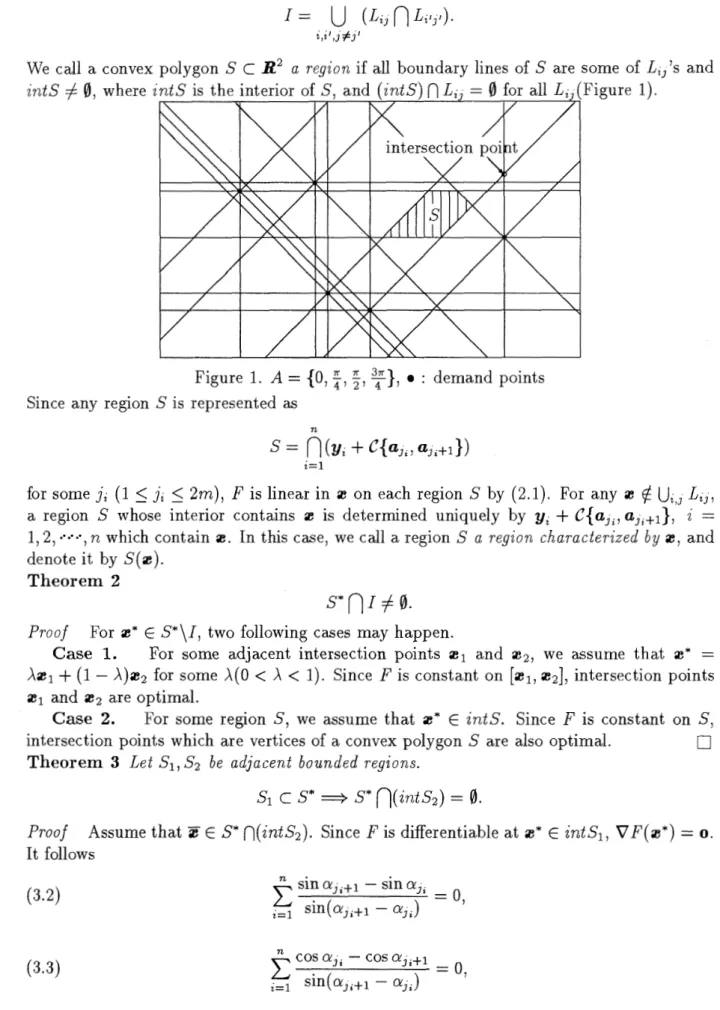
jl, we call a point Lij Liljl a n i n t e r s e c t i o n point. Let I be a set of intersection points, i.e.

We call a

zntS

#

0,

convex polygon S C IZ2 a region if all boundary lines of S are some of where

Lij7s and

-1.

Figure l . A =

10,

:, :,

21,

e : demand points Since any region S is represented as

for some ji (l

5

ji

5

2m),

F

is linear in

z

on each region S by (2.1). For any z

$

UiIi Lij,

a region S whose interior contains z is determined uniquely by yi

+

C{aji,

aji+l}, z =

l7 2,

,

n which contain z . In this case, we call a region S a region c h a r a c t e r i z e d b y z , and denote it by S ( z ) .

Theorem 2

s * ~ I + o .

Proof For z* E S*\I, two following cases may happen.

Case l. For some adjacent intersection points z l and Azl

+

(1 - A)z2 for some A(0

<

A

<

1). Since

F

is constant on zl and z 2 are optimal.

Case 2. For some region S, we assume that z* E zntS.

z2, we assume that X * =

[zl, z2], intersection points Since

F

is constant on S, intersection points which are vertices of a convex polygon S are also optimal. _U

Theorem 3 L e t Sl, S2 be a d j a c e n t b o u n d e d regions.

Proof Assume that Z E S* n(zntS2). Since

F

is differentiable at

z*

E intSl,

V F ( z * )

= 0 ,

It follows (3.2)

(3.3)

5

sin aji+l - sin aji

Location Problem under The A-Distance 13

for some 3i ( l

5

3;

5

2m). Let X I , x2 be end points of a line segment Sl

n

S2 and ajo ( l

5

jo

5

m) be an orientation of a line which passes x l and x2. We set Iajo =

{ i

: y i = X 1

+

332

2

+

yajo for some y

>

0, l

5 i 5

n

I

l

=

{ i

y i = X 1

+

332

'am+~O

2

+

yam+j0 for some y

>

0, l

5 i

5

n

I

.

Note that

I a J o U I a m + J o

#

0.

For

i

â I a J o , (a) X* E Yi+c{am+J~,am+jo+l} or (b) X *

c

Yt

+

c{am+jo -1 7 am+jo

} holds. It is sufficient to show the case (a). We assume that the case

(a) holds.

Figure 2 .

From (3.2) and (3.3),

sin aji+l - sin aji

X

wi

.

+

X

wi Sin am+ jo +I Sin a m + j o

2 Qaj0

U

I c ~ ~ + ~ ~ ~ l ~ ( ~ j i + l aji) i c ~ ~ . JO sin(am+j0 +I - am+jo

)

COS aj0 -1 COS aj0

+

wi = 0.

~ ~ I a m + j o sin(aio - aio - l ) Therefore VF(Z) can be represented as

For i

c Iajo,

V ~ A ( X * , Yi)

c

infc{am+jo 7 am+jo +I}, V ~ A

(z,

'Yi) intc{am+jo -1 7 am.+jo

}-

For

i

c

Ia m+jo l

14 M. Kon & S. Kushjmoto

and

we have

Thus E is not optimal. This contradicts the assumption.

0

Let {PA, A E A} be a set of all convex polygons such that they include all demand points and their all boundary lines are A-oriented lines, where A is an index set. We set

P is the smallest convex polygon such that it includes all demand points and its all boundary lines are A-oriented lines(Figure 3). Note that boundary lines of P are A-oriented supporting lines to { Y ~ , y2,

.

Figure 3. P for {pl, y 2 ,

- ,

y5}, A = {0,

2,

:,

9 )

Theorem 4

S*

c

P.

Prooj We assume that E

f P

is optimal. There exists a line

L

such that

L

is an A-oriented supporting line to P and separates Z from

P

and E i s not on

L.

By the rotation of the plane and the translation, without loss of generality, we assume that Z is the origin and

L

is y = c

for some c

>

0. According to such rotation and translation, we transform A-orientations and reset a ~ , a 2 ,

,

am. Note that {gl, y2,

. . ,

yn} C {(X, y ) : y

>

0} and a1 = 0. For

each y i , yi E C{aji, aji+l} for some ji (l

5

ji

5

rn- l) and y i is not on a line y = 0. Now we consider the A-circle with radius d A ( z , yJ at center y i . For the simplicity of the notation, we set

(i) w h e n 9; E intC{aji, aji+1} for some j; ( l

5

j i

5

na - l), for su%ciently small E

>

0 and any

Location Problem under The A-Distance

we have

dA ( W a , y,)

<

dA (5% y,).

(ii) When y, = 70,. for some 7

>

0, ji (2

<

ji

<

m), for sufficiently small E

>

0 and any a E {ie E f 1 2 : (cos&.l, .cT

<

O}

n

{ie E f i 2 : (cos

bi,

sinpji) .cT

<

O}

,

we have

d ~ ( x + &a, YZ)

<

dA(5, Y ~ ) .

Since _m

(0,1) E

0

{.B E : (cos

p,,

sin@,) ieT

<

0}

,

,=l we have

d ~ ( z + ~ ( 0 , I ) , y , )

<

d ~ ( a ' , y , ) , i = 1 , 2 , - - - , n for sufficiently small E

>

0. Therefore

F@+ ~ ( 0 , l))

<

F ( 4 .

This contradicts the assumption. D

By Theorem 2 and 4, there exists an optimal solution which is an intersection point in P. So we consider the determination of such an optimal solution by the iterative method that traces only intersection points in P, where an initial point is any demand point. Now we assume that we have a point .E(") after r t h iteration. Note that ie^ E I. We say a,

satisfies condition (Q) for

x^

if

3yi s.t. y i = a'(")

+

70, for some 7 6

R

and We set

3e

>

0 s.t. US'-')

+

e a j E P.

J = { j : aj satisfies condition (Q) for idT).}.

For the objective function F, we represent the right differential coefficient of F at XQ E

f 1 2 with respect to o

#

a 6 f 1 2 as 9+F(ieo; a), and set

If U ^

>

0, then

x^

is optimal by the convexity of

F.

By Theorem 3, 4 and the proof of Theorem 3, S* is an intersection point or an A-oriented line segment whose end points are adjacent intersection points or a region.

Before we state an algorithm, we consider the determination of P. We sort Lij's according to X-intercept or y-intercept. For each aj, if

a,

#

-,

then

L+

is - X tan oj+ y = y]- y} tan aj and we set bij = y; - y: tan a,. Otherwise Lij is X = IJ] and we set bij = y:. For each j, we

sort all different lines among Lij's according to 6;:s in ascending order. Let

<,

g,

-

,

be those lines, where

t\

is the ith line among &,-oriented sorted lines. Note that n j

<

n.

7T 7T

Now we assume that 0

<

a1

<

<

<

5,

a^, = 5,

<

<

<

am

<

T . We

16 M. Kon & S. Kushlmoto

The kth line in (3.5) is ak-oriented^ = 1 , 2 , ' - . , 2 m ) . It is the bottom line if 1

<

k

<

q - 1 or m

+

q

<

k

<

2m, and it is the top line if q

<k

<

m

+

q - 1. The top line means the northmost or eastmost line among drawn lines with a same orientation, and the bottom line means the southmost or westmost line among drawn lines with a same orientation. Note that an am+.-oriented line is also an aj-oriented line ( j = l, 2,

,

m). In ( 3 . 5 ) ,

lf

'S are

arranged as if they wrap

P

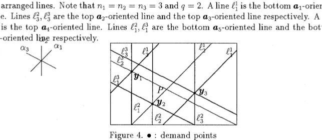
counterclockwise. The complexity for sorting n real numbers is O(n log n) [l]. So the complexity of the above sorting is O(n log n).

For example, we consider the case n = 3, m = 3(Figure 4). We have

as arranged lines. Note that nl = n2 = n3 = 3 and q = 2. A line l: is the bottom al-oriented line. Lines lg,l: are the top a2-oriented line and the top %-oriented line respectively. A line

&

is the top a,-oriented line. Lines

g,

are the bottom as-oriented line and the bottom ae-oriented 1QW respectively.

"^l

Figure 4. : demand points

Now coefficients of Li3's are stored. When we consider P,

"="

in

i\

(1

<

j

<

m) is replaced by

">",

and

"="

in ^ ( l

<

j 5 m) is replaced by "5".

P

is a region determined by its system of inequalities. Note that this system of inequalities may contain redundant inequalities.

For the simplicity of the notation, let ^ ( l ) , l(2),

.

,

l(2m) be lines in (3.5). Especially, we set @m

+

1) = l(1) and <{2m

+

2) = l(2).

The procedure for the determination of

P

Step 1. Determine an intersection point of l(1) and l(2), and let zl be its intersection point. Set j = 2.

Step 2. Determine an intersection point of

l(j)

and / ( j

+

l), and let z, be its intersection point.

Step 3. If

zi

= z j _ ~ then remove l ( j ) .

Step 4. If j = 2m

+

1 then stop otherwise set j = j

+

1 and go to Step 2.

Let

lid,

l(j2),

,

Q,)

be lines left after the above procedure. P is represented by a system of inequalities corresponding to those lines. Now its system of inequalities does not contain redundant inequalities.

The Edge Tracing Algorithm

Step 1. Choose any demand point as an initial point

do).

(We choose a demand point with the largest weight

.)

Set r = 0.

Step 2. Calculate d T ) .

Step 3. If U^

>

0 then stop.

idT)

is an optimal solution.

Step 4. 1f U^ = 0 then stop. If the number of a k 7 s which satisfy U(') = 0, i.e. 9 + ~ ( a s ( ~ ) ; ak) =

Location Problem under The A-Distance 17

1. one, then any point a* ? [a*^), zfc], where a?" is an ak-oriented adjacent inter-

section point to a*^), is optimal.

2. two, then for sufficiently small e

>

0 and a k l , ak2 which satisfy

u^

= 0, any point a* E

S(Z(^

+

e(akl

+

at,)) is optimal.

Step 5. Otherwise, i.e. U^

<

0, choose any a k which satisfies U(') = Q + F ( z ( ' ) ; a^), and

let a*("+') be an ak-oriented adjacent intersection point to X^. Set r = r

+

1, and go to Step 2.

The Edge Tracing Algorithm is convergent in finite iterations because a*(') in The Edge

Tracing Algorithm is different from a^'), a*('), S-- , a*('^ and the number of intersection

points is finite and F(z('))

>

F(z('))

>

>

F(a(')) from Step 5. The number of intersection points is 0 ( n 2 ) . For a given a* ? .E2, the complexity for calculating F ( z )

is 0 ( n ) , so the complexity for determining U(') in Step 2 is O(n). The complexity for

determining S(Z^

+

s-{aki

+

ak2)) in 2 of Step 4 is 0 ( n ) , so the complexity of Step 4 is 0 ( n ) . The complexity for determining is O(1) when we have sorted lines, so the complexity of Step 5 is O(1). Therefore the complexity of The Edge Tracing Algorithm is 0 (n3).

If a k which satisfies U ( ' ) =

a+

F(z('); a k ) is determined in Step 5 of The Edge Tracing

Algorithm, we need to determine z('+') which is an ak-oriented adjacent intersection point to a*('). Next we consider the procedure to determine &+l). For each j, let fj(x, y) be the

left side of Lã i.e.

If a,

#

£

then V fj(x, y) =

(-

tan&,, l), otherwise V fj(x, y) = (1,O).

We assume that an initial point

ad0)

= y , is given. Set r = 0 where r is a counter. We

corresponding to Lig/s (e.g. binary search). Note that a*^ is an intersection point of <r,j)'s,

i.e. a*(') can be represented by sT(j)'s. We concentrate on ~ ~ ( 7 ) ' s . We assume that a k in

Step 5 is determined. Set

/ =

i f l < k < m ,

k - m i f m < k < 2 m .

where

<

-,

>

is the inner product, and we determine an intersection point of ^Jj0 and

18 M. Kon & S. Kushimoto

' E J ^ ) . Set

&+l) is an intersection point of th and ~ r ( _ , ) + s , g n ( t k , ) , J

ST

U)

if j = ji,

(3.8) S,(])

+

sign(tkj) if j E J('\

S, (j)

+

0.5sign(tki) otherwise.

Set r = r

+

1, and go to Step 2.

Now, a point a*^ is an intersection point of < , ' S such that sT (j) G N where N is a

set of natural numbers. For j such that s T ( j )

$

W ,

it means that a*^ lies between i\sr(i)l

and ~ s r , j ) l + l where [ a ] is Gauss' symbol.

In The Edge Tracing Algorithm, we represent a point a*(T) after the r t h iteration as

The above representation is only the case of r = 0. If we consider the case of r

>

1, s T ( j )

+

sign(tkj) in (3.6) and the second equation in (3.8) is replaced by

and sign(tkj) in the third equation in (3.8) is replaced by

4. Numerical Example

We consider a single facility minisum location problem rnin F(z)

xeR2

where F ( x ) = _{dA(z, yi), A = {0,}

_{f ,}

_;,

y } ,

_{y l = (63,97), y 2 = (102,7), y, = (10, go),}

y4 = (197,57), y, = (73,20). In this case, n = 5 and wl = w 2 = WJ = w4 = w s = 1. We set

a*(') = y as an initial point, and apply The Edge Tracing Algorithm to this problem.

1. (Step 1) The initial point is a*(') = (63,97) with

Go to Step 2.

2. (Step 2) We have U(')

<

0. Go to Step 5.

3. (step 5) We have k = 7, so

x^

is an ay-oriented adjacent intersection point t o

x^.

Go to Step 2.

4. (Step 2) We have

dl)

= (63,90) with

Continuing the above procedure, we have = (63,57), a*(^ = (73,57), a*'-^ = (73,36), and

U^

>

0. The optimal solution is a*(*) = (73,36), and the optimal value is F(* = 340.22

Location Problem under The A-Distance

Figure 5.

0

: the optimal solution, m : demand points

5 . Conclusion

We considered a single facility minisum location problem under the A-distance, This problem can be used when the facility to be located is the public one. In this case, we can regard the A-distance as the approximation to the road distance, and demand points as locations of users of the facility, and each weight as the number of users in the location of the demand point. We showed that at least one optimal solution is an intersection point(Theorem 2) and any optimal solution belongs to P(Theorem 4). A set of optimal solutions is an intersection point or an A-oriented line segment or a region by Theorem 3 and 4. Based on these results, we proposed The Edge Tracing Algorithm to determine all optimal solutions. The Edge Tracing Algorithm is an iterative algorithm using the descent method. Its algorithm generates a finite sequence of intersection points converging to an optimal solution. We also proposed the method of determining the next point efficiently in its algorithm by sorting drawn lines. We chose the demand point with the largest weight as an initial point. But we may need many iterations if the initial point is not near to an optimal solution and there are a lot of demand points near the optimal solution. In this sense, we need further research on the choice of an initial point to find an optimal solution more efficiently.

References

A. V. Aho, J.E.Hopcroft and J.

D.

Ullman, "The Design and Analysis of Computer Algorithms"

,

Addison- Wesle y, Reading, MA, 1974, 65-67

Z. Drezner and A. J. Goldman, "On the Set of Optimal Points to the Weber Problem", Trans. Sci., Vol.25, No.1, 1991, 3-8

Z. Drezner and G. 0 . Wesolowsky, "The Asymmetric Distance Location Problem", Trans. Sci., Vol.23, N0.3, 1989, 201-207

H. Konno and H. Yamashita, "Nonlinear Programming" (in Japanese), Nikkagiren, Japan, 1978

S. Kushimoto, "The Foundations for the Optimization" (in Japanese), Morikita Syup- pan, Japan, 1979

T. Matsutomi and

H.

Ishii, "Facility Location Problem with Restricted Orientations" (in Japanese), RIMS Kokyuroku 798, 1992, 129-139

2 0 M. Kon & S. Kushimoto

[g] S. Shiode and

H.

Ishii, "A Single Facility Stochatic Location Problem under A-

Distance", Ann. Oper. Res., Vol.3 l, 1991, 469-478

[g] J. E. Ward and R. E. Wendell, "Using Block Norms for Location Modeling'', Oper. Res., Vo1.33, 1985, 1074-1090

[l01 J. E. Ward and R. E. Wendell, "A New Norm for Measuring Distance Which Yields Linear Location Problems", Oper. Res., Vo1.28, N0.3, 1980, 836-844

[ll] R. E. Wendell, A. P. Hurter, Jr. and T. J. Lowe, "Efficient Points in Location Prob- lems", AIIE Trans., Vo1.9, N0.3, 1977, 238-246

[l21 P. Widmayer, Y. F. Wu and C. K. Wong, "On Some Distance Problems in Fixed Orientations", SIAM J. Comput., Vo1.16, 1987, 728-746

Masamichi Kon

Department of Mathematics, Faculty of Education, Kanazawa University, Kakuma, Kanazawa, Ishikawa, 920-1 l, Japan

[email protected] Shigeru Kushimoto

Department of Mathematics, Faculty of Education, Kanazawa University, Kakuma, Kanazawa, Ishikawa, 920- l l, Japan