SYNOPTIC TRANSPORT MODELING IN THE CA RIVER BASIN, NORTH CENTRAL VIETNAM
Ho Thi Phuong
Graduate School of Environmental and Life Science (Doctor’s Course)
OKAYAMA UNIVERSITY
September 2019
TABLE OF CONTENTS
Page
LIST OF FIGURES ... iv
LIST OF TABLES ... vi
ABSTRACT ... 1
CHAPTER 1. CA RIVER BASIN ... 3
1.1. NATURAL CHARACTERISTICS ... 3
1.1.1. Topographic ... 3
1.1.2.Vegetation cover and soil ... 4
1.1.3.Climate ... 5
1.2.SOCIO-ECONOMIC CHARACTERISTICS ... 7
1.3.RUNOFF AND RESERVOIRS ... 8
1.3.1.Runoff ... 8
1.3.2.Reservoirs ... 9
REFERENCES ... 9
CHAPTER 2. SYNOPTIC MODEL ... 11
REFERENCES ... 12
CHAPTER 3. A HYDROLOGICAL TANK MODEL ASSESSING HISTORICAL RUNOFF VARIATION ... 13
3.1. INTRODUCTION ... 13
3.2. STUDY AREA AND DATA SOURCE ... 13
3.2.1. Study area ... 13
3.2.2. Data ... 14
3.3. METHODS ... 15
3.3.1. Rainfall-runoff analysis ... 15
3.3.2. Assessment of hydrological regime change ... 17
3.4. RESULTS ... 18
3.4.1. Evaporation data extension ... 18
3.4.2. Change points of annual precipitation and discharge... 19
3.4.3. Trial of tank model calibration for the whole period of 1962–2014 ... 21
3.4.4. Tank model calibration for the first period (1962–1983) at Quy Chau station ... 23
3.4.5. Tank model calibration for the first period (1973–1983) at Nghia Khanh station .. 24
3.4.6. Tank model validation ... 25
3.5. DISCUSSION ... 27
3.5.1. Tank model calibration using monthly input data ... 27
3.5.2. Temporal change of runoff at the Upper Hieu River ... 28
3.6. CONCLUSIONS ... 30
REFERENCES ... 31
CHAPTER 4. EFFECTS OF DAM CONSTRUCTION ON TOTAL SOLIDS ... 33
4.1. INTRODUCTION ... 33
4.2. STUDY AREA AND DATA ... 34
4.3. METHODS ... 35
4.3.1. Station hydraulic geometry ... 35
4.3.2. Calculation of suspended sediment load ... 36
4.3.3. Efficiency criteria used for calibration and validation of simulated suspended sediment load ... 37
4.3.4. Electrical conductivity and total dissolved solids ... 38
4.4. RESULTS AND DISCUSSION ... 39
4.4.1. Hydraulic geometry characteristics at the cross-sectional scale ... 39
4.4.2. Calibration and validation of the suspended sediment load ... 41
4.4.3. Change in the relationship between sediment particle size and channel roughness 43 4.4.4. Impact of a reservoir on suspended sediment yield ... 44
4.4.5. Long-term TDS yields and changes in the TSS-to-TDS ratio ... 45
4.5. CONCLUSIONS ... 47
REFERENCES ... 48
CHAPTER 5. GEOCHEMISTRY AND SEDIMENT: WEATHERING PROCESS, SOLUTE-DISCHARGE RELATIONSHIP, AND RESERVOIR IMPACT ... 50
5.1. INTRODUCTION ... 50
5.2. STUDY AREA ... 50
5.3. SAMPLING AND ANALYTICAL METHODS ... 51
5.4. RESULTS AND DISCUSSION ... 52
5.4.1 The contribution of chemical compositions ... 52
5.4.2. Spatial and seasonal variations of major solutes and suspended solids ... 55
5.4.3. Weathering processes controlling the major ion chemistry ... 57
5.4.4. Variations of major solute concentration with discharge ... 61
5.4.5. Primary evidence of reservoir impact on suspended solids and dissolved solids concentration ... 63
5.6. CONCLUSIONS ... 65
REFERENCES ... 66
CHAPTER 6. CONCLUSIONS ... 69
ACKNOWLEDGEMENTS ... 70
LIST OF FIGURES
Figure 1.1. Ca River basin ... 3
Figure 2.1. Synoptic model ... 12
Figure 3.1. Location of the Hieu River basin ... 13
Figure 3.2. Structure of the tank model ... 16
Figure 3.3. Correlation between mean monthly Em/P and mean monthly P ... 18
between 1962 and 2014 ... 18
Figure 3.4. Correlation between annual Ep and annual Ea between 1962 and 2014 ... 19
Figure 3.5. Cumulative anomaly test results of annual rainfall (a), annual discharge at Quy Chau station (b) and annual discharge at Nghia Khanh station (c) ... 20
Figure 3.6. Mean annual rainfall (a), mean annual discharge at Quy Chau station (b) and mean annual discharge at Nghia Khanh station (c); break points are identified ... 21
Figure 3.7. Calibrated tank model (a) at Quy Chau hydrological station for 1962–2014 and (b) at Nghia Khanh hydrological station for 1973–2014 ... 22
Figure 3.8. Calibrated tank model at the Quy Chau gauging station from 1962–1983 ... 24
trial No. 1 and (b) trial No. 2 ... 24
Figure 3.9. Duration curves at Quy Chau station from 1962–1983 ... 25
(a) trial No. 1 and (b) trial No. 2 ... 25
Figure 3.10. Calibrated tank model at Nghia Khanh station from 1973–1983 ... 26
(a) trial No. 1 and (b) trial No. 2 ... 26
Figure 3.11. Duration curves at Nghia Khanh station from 1973–1983 ... 27
(a) trial No. 1 and (b) trial No. 2 ... 27
Figure 3.12. Calibrated parameters of the tank model using monthly data ... 28
Figure 3.13. Double mass curves of precipitation and discharge ... 29
Figure 4.1. Map of the Ca River ... 35
Figure 4.2. Relationship of width, depth, and velocity to discharge ... 40
at Dua (a) and Yen Thuong (b) ... 40
Figure 4.3. Comparison of observed and calculated sediment load ... 42
at Dua (a) and Yen Thuong (b) ... 42
Figure 4.4. Loading curves at Dua and Yen Thuong compared with Kazama et al. (2005) and Camenen and Larson (2008) ... 43
Figure 4.5. The relationship between sediment particle size and channel roughness during the pre-dam and post-dam periods ... 44
Figure 4.6. Observed SS load during the pre-dam and post-dam periods ... 45
at Dua (a) and Yen Thuong (b) ... 45
Figure 4.7. Long-term electrical conductivity at the Dua station ... 46
Figure 4.8. Loading curve of total dissolved solids at the Dua station... 46
Figure 5.1. Map of the Ca River basin ... 52
Figure 5.2. Seasonal variations in the concentration of ... 56
major ions (µM), TDS, and SS (mg/l) ... 56
Figure 5.3. Monthly variations in the concentration of TDS and SS (mg/l) ... 56
Figure 5.4. The Gibbs graph of Ca River between the ratio of Na/(Na+Ca) ... 57
and total dissolved solids ... 57
Figure 5.5. Scatter plots between (a) Ca2+ and HCO3-, (b) Ca2+, Mg2+, and total cations, and (c) Na+, K+, and total cations ... 59
Figure 5.6. Piper trilinear diagram of Ca River water in comparison with other river basins . 60 (data from Ding et al. 2016; Fan et al. 2014; Liu et al. 2018; Maharana et al. 2015) ... 60
Figure 5.7. Variation of river elements concentration with discharge ... 62
at My Ly (a, b), Dua (c, d), and Yen Thuong (e, f) ... 62
Figure 5.8. Variation of suspended sediment concentration with discharge ... 63
at My Ly (a), Dua (b) and Yen Thuong (c) ... 63
LIST OF TABLES
Table 1.1. Average temperture of many years in the Ca River ... 5
Table 1.2. Average humidity of many years in the Ca River ... 6
Table 1.3. Average rainfall of many years in the Ca River ... 7
Table 1.4. The annual flow of many years at selected stations in the Ca River ... 8
Table 1.5. Major reservoirs in the Ca River (Chikamori et al. 2012) ... 9
Table 3.1. Nash-Sutcliffe efficiency (NSE) and the coefficient of determination (R2) resultsfor different time periods ... 27
Table 4.1. The exponents and coefficients of at-a-station hydraulic geometry parameters ... 39
Table 4.2. Calibration and validation results of the suspended sediment load at n = 0.015 .... 41
Table 5.1. Chemical compositions of the rivers in the Ca River basin ... 53
Table 5.2. Correlation matrix of measured parameters at three hydrological stations ... 58
ABSTRACT
The study was performed in the Ca River basin, which is the third largest river in north-central Vietnam, located between 18°15′00′′N and 20°10′30′′N and 103°45′20′′E and 105°15′20′′E. Ca River basin covers an area of 27,200 km2 in which the area in Vietnam territory is 17,730 km2, holding 65.2% of the total drainage area. The trunk river length is 531 km, of which 170 km runs through Lao PDR and 361 km runs through Vietnam. Ca River, like many other rivers around the world, have been impacted by economic development.
Various sized reservoirs have been constructed along the rivers for power generation, water supply, and flood control. In addition, other anthropogenic activities (e.g., intensive agriculture, land-use change, and industrial development) may disrupt the dynamic equilibrium between the movement of water and the movement of sediment that exists in free- flowing rivers, resulting in an alteration of natural river regimes, a modification of a river’s morphology and riverbed characteristics, and a change in ion constitution. The aim of dissertation thesis is to examine the degree of human-induced alteration of the natural flow regime and the material budgets in the Ca River basin using Synoptic model include the Tank model, regime law and resistance law.
The Hieu River is the largest tributary on the left bank of the Ca River. Here, we use cumulative anomaly tests and Pettitt tests to ascertain the turning points in annual rainfall and discharge during the time period 1962–2014. The results of our statistical analysis reveal a breaking point in 1982 for the rainfall time series and in the late 1970s and late 1990s for the discharge time series. A storage-type hydrological model is used to determine runoff processes for different periods corresponding to detecting points of rainfall and discharge. The results of our model simulation confirm that a two-tank model with monthly input data is the most appropriate tank model for the Hieu River. The difference between the hydrographs improved when we used a rain factor as a function of the month. A comparison between the observed and calculated runoff revealed a drastic decrease between 1999 and 2014. The rate of discharge loss in the Lower Basin was approximately six times higher than that in the Upper Basin, a finding potentially due to reservoir construction and intensive water use for agricultural and residential purposes.
The river regime laws of the hydraulic properties of the cross sections of two hydrological stations (Dua and Yen Thuong) along the Ca River were combined into power functions with exponents of 1.46–1.85 using the Manning roughness coefficient and the
settling velocity or the particle size to simulate the suspended sediment load. The Nash- Sutcliffe efficiency, percent bias, and the ratio of the root-mean-square error to the standard deviation of the measured data were used to evaluate the calibration process for the pre-dam period (1994–2004) and for validation for the post-dam period (2005–2014). Effects of dam construction include a change in the relationship between the Manning roughness coefficient and sediment particle size. The observed sediment load decreased by approximately 20–40%
after dam construction at both stations. We used a power function with exponents of 0.968 and 0.992 for the dissolved solid load to calculate the long-term annual total dissolved solids at the Dua and Yen Thuong stations, respectively. After dam construction, the average value of the total suspended solids-to-total dissolved solids ratio decreased from 3.0 to 2.3 at the Dua station and from 4.1 to 2.2 at the Yen Thuong station.
This study investigates the chemical composition of dissolved loads in the Ca River basin. The water samples were collected for 1 year from August 2017 to July 2018 at three hydrological stations located in the mainstream of the Ca River. We found that carbonate weathering is the dominant process controlling the water chemistry in the study area.
Bicarbonate and calcium are dominant chemical species, accounting for 84.4% and 62.0% of the total anionic and cationic charge, respectively. The average dissolved-solids concentration is 144 mg/l and generally decrease from the upstream to downstream, resulting in a decrease of the major ions in the downstream basin. The variation of major chemical ions and suspended solids concentration with discharge was also investigated. As a result, major chemical weathering products behave chemostatically, with increasing discharge in the upstream. However, the dilution behavior of solutes is shown in the midstream and downstream. The ion species of NO and PO show constant to increasing concentration in the drainage basin, indicating the additional sources of organic degradation and human activities. There is primary evidence that water storage for the reservoirs has impacted on a variation of suspended solids and dissolved solids in the Ca River.
CHAPTER 1. CA RIVER BASIN
1.1. NATURAL CHARACTERISTICS 1.1.1. Topographic
Figure 1.1. Ca River basin
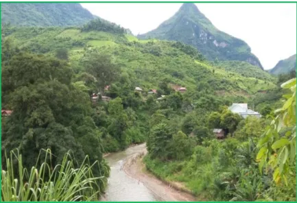
The Ca River basin is an international river, located between 18o15’00”N to 20o10’30”N and 103o45’20”E to 105o15’20”E (Figure1.1). The basin covers an area of 27,200 km2, including 17,730 km2 in Vietnam’s territory and 9470 km2 in Laos. The main river originates from Mt. Muong Khut and Muong Lap at an elevation of 1800 to 2000 m in Laos.
The river enters into the NgheAn province at Keng Du and flows to the Eastern Sea at the Cua Hoi estuary. The Ca River bed is very narrow, with steep slopes in the upstream area, it then widens up in the middle basin (from Con Cuong to Anh Son), and finally joins the Hieu River on its left side. In the downstream area, the Ca River flows through the plain and joins the La River on the right side.
The entire upstream in Lao PDR has an average altitude of over 1000 meters. In Vietnam, more than 80% of the basin area is mountainous. The length of the main Ca river is 531 km in total, of which 361 km is in Vietnam and its mean elevation is 294 m a.s.l. .
Hieu River is the largest tributary on the left side of the Ca River. The catchment area of the Hieu River is 5340 km2, its length is 228 km and originates from Pu Hoat Range in the Laos Vietnam boundary. This then flows into the Ca River at Anh Son.
La River is the main tributary on the right side of the Ca River: it originates from the Giai mountainous area and enters into Ca river at Cho Trang. The catchment area of the La River is 3210 km2.
Picture 1.1. Midstream of Ca river
(Taken in Dua hydrological station on June 28, 2016) 1.1.2.Vegetation cover and soil
According to the land survey in 2010, the structure of the land on the Vietnam territory is as follows:
1,418,053 ha of agricultural land
1,085,897.9 hectares of forestry land
158,518,4 ha of non-agricultural land
386,092 ha of unused land.
The vegetation cover on agricultural land is estimated to be at 20–25%. Forests in the Ca River basin are largely located in the upstream of three Laos provinces (Bolikhamxay, XiengKhouang, and Houaphanh). In Vietnam, the forest is concentrated in the north, northwest, and southwest of the basin at an elevation of 150 to 1500 m (IWRP 2012). The natural land is mostly evergreen and semi deciduous tropical forest, although mixed forests can be found in some areas (Giang et al. 2014).
Before 1995 the forest in the Ca river basin was rapidly reduced due to exploitation and poor maintenance. According to the forest inventory data of the Ca River basin in Vietnam, in 1943 there was about 1.2 million ha of forest and in 1999, the forests were only about 710,000 ha. The coverage was 35.5%. From 1995 to 2010 the forest in the basin has started to be preserved and restored due to rapid forest plantations and land and forest
allocation. This combined with the mountainous economic development programs has made the current forest in Nghe An rise to 51.5% coverage and Ha Tinh has reached 50.2%.
The soil in this area is formed from parent rocks, mainly Ferralsol accounting for 83.51% (IWRP 2012; Nauditt and Ribbe 2017). Other soil types are Fluvisol and Acrisol.
Picture 1.2. Forest cover in moutainous area of Ca river (Taken in My Ly catchment on August 13, 2017) 1.1.3.Climate
a/ Temperature
Table 1.1. Average temperture of many years in the Ca River
Stations Months Ave
(oC) Jan Feb Mar Apr May Jun Jul Aug Sept Oct Nov Dec
Con Cuong 17.1 18.0 20.4 24.5 27.0 28.1 27.7 27.2 25.9 23.2 20.2 18.4 23.1 Cua Rao 16.9 18.9 21.7 25.0 26.8 27.5 27.1 26.7 25.7 23.6 20.0 17.7 23.1 Do Luong 17.8 18.5 20.9 24.5 27.5 29.1 29.1 28.1 26.7 24.5 21.6 18.8 23.9
Ha Tinh 16.7 17.7 20.4 24.5 27.1 28.8 28.8 27.0 25.4 23.8 20.9 18.4 23.3 Huong Khe 19.2 20.1 22.4 25.9 28.5 29.7 29.6 29.3 27.4 25.3 22.8 20.2 25.0 Huong Son 17.2 17.9 20.4 24.3 27.8 29.5 29.4 28.9 27.8 25.4 22.2 18.8 24.1 Kim Cuong 16.2 17.3 19.9 23.9 27.6 29 28.9 28.5 27.4 24.8 21.6 18.3 23.6
Ky Anh 18.0 19.5 21.4 25.2 27.8 30.4 30.1 28.8 27.0 25.4 22.3 19.4 24.6 Quy Chau 15.2 17.2 19.7 23.9 26.0 26.9 27.0 26.2 25.1 23.1 19.2 15.4 22.1
Quy Hop 17.9 19.1 21.6 25.2 27.4 28.5 28.9 27.9 26.4 24.6 21.6 18.6 24.0 Quynh Luu 17.1 18.0 19.9 23.4 26.7 28.1 28.4 27.4 26.2 23.3 19.8 18.4 23.1
Tay Hieu 17.0 18.1 20.7 24.5 27.2 28.6 28.7 27.6 26.3 24.0 21.0 17.9 23.5 Vinh 17.6 18.2 20.6 24.2 27.8 29.6 29.7 28.7 26.9 24.6 21.8 18.8 24.0
The Ca River basin is located in a monsoon climate, with two distinct seasons: the wet and dry seasons. The wet season, starting from May to October, is hot and humid due to the southwest monsoon (locally called the Laos wind). The dry season lasts six months from November to April which is cold and dry caused by the northeast monsoon. The temperature of the plain is higher than the midland and mountainous areas. This is shown in the average temperature of Vinh 23.8oC, Do Luong 23.7oC, Tuong Duong 23.6oC and Tay Hieu 23.2oC (Table 1.1).
b/ Humidity
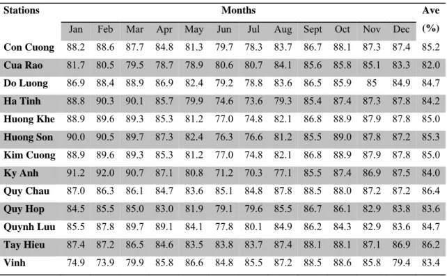
The annual average humidity in the Ca River basin ranges from 82% to 85%.
Humidity corresponds to the evaporation of the year. The middle of the basin with high humidity corresponds to low evaporation, and mountainous areas and the plain has high evaporation corresponding to low humidity. The highest monthly humidity reach up to 94% in January and February, the lowest humidity is in July (Table 1.2).
Table 1.2. Average humidity of many years in the Ca River
Stations Months Ave
Jan Feb Mar Apr May Jun Jul Aug Sept Oct Nov Dec (%)
Con Cuong 88.2 88.6 87.7 84.8 81.3 79.7 78.3 83.7 86.7 88.1 87.3 87.4 85.2 Cua Rao 81.7 80.5 79.5 78.7 78.9 80.6 80.7 84.1 85.6 85.8 85.1 83.3 82.0 Do Luong 86.9 88.4 88.9 86.9 82.4 79.2 78.8 83.6 86.5 85.9 85 84.9 84.7 Ha Tinh 88.8 90.3 90.1 85.7 79.9 74.6 73.6 79.3 85.4 87.4 87.3 87.8 84.2 Huong Khe 88.9 89.6 89.3 85.3 81.2 77.0 74.8 82.1 86.8 88.9 87.9 87.8 85.0 Huong Son 90.0 90.5 89.7 87.3 82.4 76.3 76.6 81.2 85.5 89.0 87.8 87.2 85.3 Kim Cuong 88.9 89.6 89.3 85.3 81.2 77.0 74.8 82.1 86.8 88.9 87.9 87.8 85.0 Ky Anh 91.2 92.0 90.7 87.1 80.8 71.2 70.3 77.1 85.5 87.4 86.9 87.5 84.0 Quy Chau 87.0 86.3 86.1 84.7 83.6 85.1 84.8 87.8 88.5 88.0 87.2 87.2 86.4 Quy Hop 84.5 85.5 85.0 83.0 81.9 79.1 79.6 85.5 86.7 86.1 82.9 83.8 83.6 Quynh Luu 85.5 87.8 89.7 89.1 84.1 77.8 80.1 84.9 86.2 84.3 82.9 83.6 84.7 Tay Hieu 87.4 87.2 86.5 84.6 83.5 83.8 83.7 87.4 88.1 88.1 87.1 86.9 86.2 Vinh 74.9 73.9 79.9 85.8 86.6 84.8 85.5 87.2 88.5 88.6 85.8 79.4 83.4
c/ Rainfall
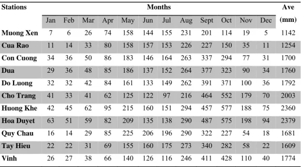
Mean annual precipitation in the basin ranges from 1100 mm in the upstream mountain area to 2400 mm close to the junction with the La river. The average rainfall of the whole basin is 1800 mm. Rainfall is concentrated in one rainy season from May to October when falls 80% to 85% of annual rainfall. The heaviest rainfall occurs around September
when the mean of the maximum daily rainfall is up to 250 mm in the coastal area, and in 2010 a maximum value up to 800 mm was recorded in 24 hours (Table 1.3).
Table 1.3. Average rainfall of many years in the Ca River
Stations Months Ave
(mm) Jan Feb Mar Apr May Jun Jul Aug Sept Oct Nov Dec
Muong Xen 7 6 26 74 158 144 155 231 201 114 19 5 1142 Cua Rao 11 14 33 80 158 157 153 226 227 150 35 11 1254 Con Cuong 34 36 50 86 183 146 164 263 337 294 77 31 1700 Dua 29 36 48 85 186 137 152 264 377 323 90 34 1760 Do Luong 32 32 42 84 161 133 149 262 391 371 100 36 1792 Cho Trang 41 33 41 62 125 122 97 216 464 552 179 70 2003 Huong Khe 42 45 62 95 215 160 151 294 457 577 188 75 2360 Hoa Duyet 63 51 59 82 209 135 138 290 487 575 198 94 2379 Quy Chau 16 14 29 85 225 206 196 290 322 227 54 18 1681 Tay Hieu 22 22 31 69 155 160 175 273 340 282 58 22 1609 Vinh 26 27 38 66 140 126 116 246 411 428 110 40 1774
1.2.SOCIO-ECONOMIC CHARACTERISTICS
In this part of Vietnam the population is 3,557,963 people with a natural area of 19,626 km2 (in 2010). Population is mostly concentrated in cities, towns, and delta areas such as Vinh city, Cua Lo town, Hong Linh town and other smaller town. The population of Ca River basin is unevenly distributed. In the highlands and mountainous areas it is sparsely populated while the urban areas and the plains have high density populations. The average population density is 175 people/km2. The highest population density is 2912 people/km2 in Vinh city. Following that is 1851 people/km2 in Cua Lo town. The lowest density is 25 people/km2 in Tuong Duong district.
The total number of laborers in the whole region by 2010 is around 2,265,580 people.
In particular, laborers in the agriculture - forestry - fishery account for about 65%. Laborers in the industry and construction sectors account for approximately 12%. Laborers working on service, trade, education sectors account for about 23% of laborers.
Laborers in the age group of 20–40 account for about 30–35%, laborers in the age of 40–60 account for about 20%.
The main economy in the basin still uses agriculture as a foundation for development, but the economic structure has made positive changes in recent years. The proportion of
industry and service is increasing, the proportion of agriculture in the economy tends to decrease.
1.3.RUNOFF AND RESERVOIRS 1.3.1.Runoff
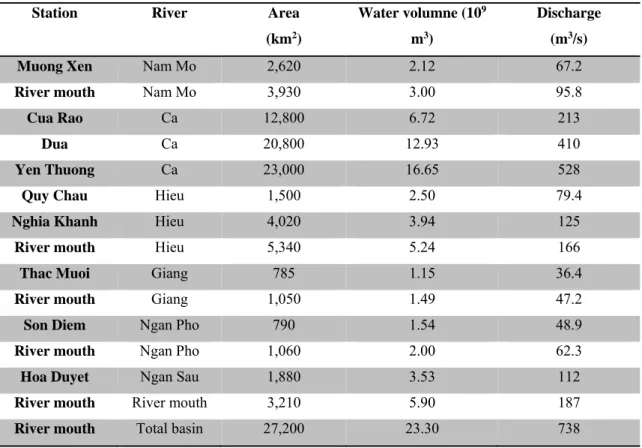
The total annual average water volume of the drainage basin is 23.3 billion m3, this corresponds to the average annual discharge of 738 m3/s. The water volume that flows in Vietnam is 17.5 billion m3, and in Laos 5.8 billion m3 of water.
Floods on Ca River have 2 distinct periods: minor floods occur in May and June and the main flood occurs in September, October and November. Floods on the Ca River's main stream and tributaries appear not at the same time.
In the main stream of the upstream of Ca River, the flood season occurs from June to the end of October (Table 1.4)
In the middle part from Dua to Yen Thuong, the flood season starts from June and ends in November
In Hieu river, the flood season starts from August and ends in November
In La river, the flood season starts from August or early September and ends later in December.
Table 1.4. The annual flow of many years at selected stations in the Ca River
Station River Area (km2)
Water volumne (109 m3)
Discharge (m3/s)
Muong Xen Nam Mo 2,620 2.12 67.2
River mouth Nam Mo 3,930 3.00 95.8
Cua Rao Ca 12,800 6.72 213
Dua Ca 20,800 12.93 410
Yen Thuong Ca 23,000 16.65 528
Quy Chau Hieu 1,500 2.50 79.4
Nghia Khanh Hieu 4,020 3.94 125
River mouth Hieu 5,340 5.24 166
Thac Muoi Giang 785 1.15 36.4
River mouth Giang 1,050 1.49 47.2
Son Diem Ngan Pho 790 1.54 48.9
River mouth Ngan Pho 1,060 2.00 62.3
Hoa Duyet Ngan Sau 1,880 3.53 112
River mouth River mouth 3,210 5.90 187 River mouth Total basin 27,200 23.30 738
1.3.2.Reservoirs
Many reservoirs have been built in the Ca River basin: the reservoirs of Ban Ve and Khe Bo on the main stream of the Ca River, the Ban Mong reservoir on the Hieu River, and the Sao River reservoir located in a tributary of the Hieu River (Table 1.5). The operation of these reservoirs, which have a total storage capacity of 2.8x10⁹ m3, an installed power generation capacity of 485 MW (excluding Song Sao) has to meet flood control with 411x106 m3 storage available, hydropower generation, water supply for irrigating 33,487 hectares, industrial, domestic and environmental demand.
Table 1.5. Major reservoirs in the Ca River (Chikamori et al. 2012)
Name of dam (reservoir)
Catchment area (km2)
Gross capacity (106
m3)
Effective capacity (106e m3)
Year of construction
Year of completion
Ban Ve 8,700 1834.6 1383 12/2005 2009
Ban Mong 2,785 252.6 125.8 5/2010 2012
Khe Bo 14,300 97.8 17.2 10/2007 12/2010
Picture 1.3. Ban Ve reservoir (Source: http://kttvqg.gov.vn)
REFERENCES
Chikamori H, Heng L, Daniel T (eds) (2012) Catalogue of rivers for Southeast Asia and the Pacific–Volume VI. UNESCO-IHP Regional Steering Committee for Southeast Asia and the Pacific. http://unesdoc.unesco.org/images/0021/002170/217039e.pdf
IWRP (2012) Synthesis report of “Review of water resources planning in the Ca River basin”
(in Vietnamese). Institute of Water Resources Planning, Directorate of Water Resources, Ha Noi
Giang PQ, Toshiki K, Sakata M, Kunikane S, Vinh TQ (2014) Modelling climate change impacts on the seasonality of water resources in the upper Ca river watershed in Southeast Asia. Scientific World Journal, 2014. http://doi.org/10.1155/2014/279135 Nauditt A and Ribbe L (eds) (2017) Land use and climate change interactions in central
Vietnam. Springer Book Series: Water Resources and Development
CHAPTER 2. SYNOPTIC MODEL
Like many other rivers around the world, Ca River has been impacted by economic development. Various sized reservoirs have been constructed along the rivers for power generation, water supply, and flood control. In addition, other anthropogenic activities (e.g., intensive agriculture, land-use change, and industrial development) may have disrupted the dynamic equilibrium between the movement of water and the movement of sediment that exists in free-flowing rivers. The aim of this dissertation thesis is to examine the degree of human-induced alteration to the natural flow regime and the material budget in the tributaries and the mainstream of the Ca River basin using the Synoptic Model.
The synoptic model consists of four parts, including configuration, hydrological, hydraulic, and operational parts. The configuration of the river basin is described by stream order theories by Strahler (1957), Shreve (1966), and Scheidegger (1968).
Firstly, the dependent variables are number, average bed slopes, average drainage area, average length of each stream order and the independent variable in the stream order.
Secondly, the regime law was shown by Leopold & Maddock (1953), where the width, depth and mean velocity of a cross-section is described by the local discharge. The regime laws are used in Chapter 4 and dimensional consideration was added.
Thirdly, as resistance laws, the friction velocity and the average velocity formulas of uniform flows are estimated as functions of the depth or hydraulic radius. The friction velocity is an essential parameter for sediment hydraulics in Chapter 4.
The last law is the Kirchhoff's to denote continuity at a confluence, a distributary and storage and release of a reservoir including water quality at conjunction. However, the configuration of the river basin and the Kirchhoff's are not investigated in this study.
The equations for n and ks are the mean velocity formulas however the velocity is given by the regime law and the closure is made. The discharge should be provided by a runoff model, and it is calculated by the hydrological tank model (as shown in Chapter 3) by the water quality routine as dissolved matters (as shown in Chapter 4 and Chapter 5). It is the form of loading equations (L-Q) of both dissolved and particulate matters, respectively.
Rating curve of water level and discharge equation (H-Q) with the duration curve of discharge ordering is all possible by using the tank model.
Figure 2.1. Synoptic model
REFERENCES
Leopold LB, Maddock T (1953) The hydraulic geometry of stream channels and some physiographic implications. US Government Printing Office, Washington
Scheidegger AE (1968) Horton’s law of stream numbers, Water Resources Res 4(3): 655–658 Shreve RI (1967) Infinite topologically random channel networks, Jour Geol 75: 178–186 Strahler AN (1957) Quantitative analysis of watershed geomorphology, Am Geophys Union
Trans 38: 913–920
CHAPTER 3. A HYDROLOGICAL TANK MODEL ASSESSING HISTORICAL RUNOFF VARIATION
3.1. INTRODUCTION
A hydrological cycle describes a water cycle, balance or budget within a drainage basin or on a global scale. Such a cycle can be affected by both natural and anthropogenic factors (Liu and Zheng 2002; Vörösmarty et al. 2000; Wang et al. 2012; Yao et al. 2015;
Zhang et al. 2001). As an inductive approach, statistical analyses and a hydrological model are effective tools to assess the impacts of natural and anthropogenic factors on the natural water cycle of the catchment. Among hydrological models, the tank model simply consists of several storage tanks arranged vertically in a series, representing a zonal structure of groundwater in the objective catchment (Sugawara et al. 1995). This study mainly focuses on the rainfall-runoff relation, and the tank model is applied to determine the runoff process that is a part of the hydrological cycle. The objective of this study was to calibrate a tank model in the large catchment lacking meteorological data. We then investigated runoff variation upstream of the Hieu River basin between 1962 and 2014 by applying the calibrated tank model.
3.2. STUDY AREA AND DATA SOURCE 3.2.1. Study area
Figure 3.1. Location of the Hieu River Basin
The Hieu River Basin is located at 19°20'N–19°50'N and 104°30'E–105°20'E, and it is the largest tributary on the left bank of the Ca River in Vietnam (Figure 3.1). The catchment area is 5340 km2 and 228 km long, and it originates from the Pu Hoat Range with an elevation of 2025 m on the Laos-Vietnam border. It flows into the Ca River at Anh Son. The mean slope is 1.3 ppt, and the average riverbed width is 30–35 m; the river network density is 0.71 km/km2. The river basin is located in the northwest of Nghe An Province, where climatic conditions are characterized by two distinct seasons: the wet season (May to October) and the dry season (November to April). This study investigates the transition of flow regime at the Quy Chau and Nghia Khanh hydrological stations located in the Upper Hieu River. The areas of Quy Chau and Nghia Khanh are 1960 and 4024 km2, respectively (Chikamori et al. 2012).
3.2.2. Data
Discharge data exist beginning from 1962 at the Quy Chau hydrological station and from 1973 at the Nghia Khanh hydrological station. Meteorological data at Quy Chau include precipitation and evaporation collected over the course of 53 years (1962–2014). All of the data were provided by the North-Central Hydro-meteorological Centre, Vietnam. Evaporation at the station was measured using a Piche tube, but evaporation data are missing for several years. Piche evaporation (Em) is converted into potential evaporation (Ep) by multiplying by factors of k1=1.263 and k2=1.107, where k1 converts from Piche evaporation to GGI-3000 evaporation according to data from Vinh station from 1961–2000 and k2 converts from GGI- 3000 to actual evaporation of the water surface (Cung, 1979; ENV, 2001).To calculate the actual evaporation of the basin, we assume that evaporation on rainy days was negligible.
Therefore, the monthly actual evaporation (Ea) was calculated by multiplying Ep by the ratio of the number of sunny days to the number of total days over a month. However, sunny day data have been available only since 1996. Therefore, the correlations among available meteorological data were investigated to extend the actual evaporation measurements from 1962–2014. The collected data revealed that the average annual precipitation and Piche evaporation at Quy Chau station were 1,668 mm and 732 mm, respectively, over 1962–2014.
The highest annual precipitation was 2,482 mm in 1978, and the lowest annual precipitation was 1,102 mm in 1976. The mean annual flow was 77m3/s between 1962 and 2014 at Quy Chau station and 126 m3/s between 1973 and 2014 at Nghia Khanh station. The annual discharge at Nghia Khanh was higher than that at Quy Chau by an average of a factor of 1.6.
The average monthly flow varied from 15–312 m3/s at Quy Chau station and from 42–334
m3/s at Nghia Khanh station. The average monthly discharge of Nghia Khanh was higher than that of Quy Chau, particularly during the flood season.
3.3. METHODS
3.3.1. Rainfall-runoff analysis 3.3.1.1. Tank model
The tank model is a conceptual representation of hydrological processes in the unit area of the basin, and it simulates wetness of several soil layers using tanks arranged vertically in a series. This kind of model typically consists of three or four storage tanks.
Precipitation is the input of the model, and it enters into the top tank.
Some of the accumulated water flows through the side outlet of a tank and some of it infiltrates down into the second lower tank. The process repeats for every lower tank.
Evapotranspiration is incorporated via subtraction from the tank. The runoff from the side outlet of a storage tank (q) is proportional to the water head over that outlet, and the infiltration (p) is proportional to the water depth. These relations can be expressed as:
, , (3.1) where h is the tank depth, z is the height of the discharge outlet from the base of each tank, a is the runoff coefficient and b is the infiltration coefficient.
In this study, the tank model with three storage tanks consisted of a surface tank, an intermediate tank, and a base tank (Figure 3.2). The two side outflows from the surface tank are regarded as the surface runoff (q11) and the sub-surface runoff (q12), the side outflow from the intermediate tank is regarded as the intermediate runoff (q2) and the outflow from the third tank is regarded as the base runoff (q3). The total outflow from the side outlet (Q) from each tank is regarded as the accumulation of the outflows from a system in the watershed, as given by the following equation:
, (3.2) where A is the watershed area.
The tank model introduced by Sugawara for humid regions includes four tanks used to analyze daily discharge from daily precipitation and evaporation inputs (Sugawara et al. 1995).
For flood analysis, the tank model includes two tanks, and the inputs are typically precipitation and the outputs are hourly discharge. Many types tank models have been developed for humid regions using daily and hourly data. Nyadawa et al. (1996) proposed a modified tank model that explicitly simulates surface runoff phenomena. These authors verified the model using data from several basins in Kenya. Kuok et al. (2011) ascertained the
best number of tanks in the tank model to provide reliable and accurate estimates of runoff for a rural catchment in a humid region. Mondal et al. (2009) applied the tank model taking into consideration soil-moisture component. Nearly all studies estimating the amount of runoff originating from the catchment area for short-term analysis using daily and hourly input data have made use of a tank model. In this study, we have simulated a tank model for long-term analyses with monthly data. A tank model using monthly data might be associated with less- complex parameters and less difficulty when considering input data for a basin lacking meteorological stations.
Figure 3.2. Structure of the tank model 3.3.1.2. Calibration of the tank model
We optimized the parameters of the tank model manually using a trial-and-error method. The value of each parameter was successively changed, and the fitness of the simulated hydrograph compared with the observed result was evaluated using the Nash- Sutcliffe efficiency (NSE):
NSE 1 ∑∑ , (3.3) where represents the observed monthly streamflow, represents the observed monthly mean streamflow and signifies the calculated monthly streamflow. In addition, the coefficientof determination (R2) was also used to evaluate the tank model.
To search for the optimal set of parameters, several principles related to the runoff and infiltration coefficients were considered. First, the sum of runoff principles related to the
runoff and infiltration coefficients were considered. The sum of the runoff and infiltration coefficients of a tank has to be less than unity (e.g., a11+a12+b1<1 in the case of the top tank).
In other words, the runoff depth from a single tank during a time increment should not exceed the water storage depth of that tank (h) (Sugawara et al. 1995; Basri 2013). Second, the runoff and infiltration coefficients of the lower tank must be smaller than those of the upper tank (i.e., a11>a12>a2). Therefore, the discharge from the lower tank is less than that from the upper tank, which reflects the fact that the discharge from a lower aquifer is typically less than that from an upper aquifer.
3.3.2. Assessment of hydrological regime change 3.3.2.1. Cumulative anomaly
The cumulative anomaly is a statistical method for the visual identification of a variable tendency of discrete data (Wang et al. 2012), and it is used extensively in meteorology. For a discrete series xi, the cumulative anomaly (Xt) for a data point xt can be expressed as
∑ , t = 1, 2,…, n, (3.4) where 1/ ∑ ; (3.5) xm denotes the mean value of the series xi; n represents the number of discrete data points. The cumulative anomaly method can be used to analyze the inflection extent of a discrete data series.
3.3.2.2. Pettitt test
The Pettitt test is a nonparametric method that is widely applied to detect abrupt changes in water discharge (Yao et al. 2015). We employed the Pettitt test using software (R;
https://www.r-project.org/). For a given time series X(x1, x2,…, xN) divided into two samples x1, x2,…, xt and xt+1, xt+2,…, xN, the Pettitt test uses a version of the Mann-Whitney statistic Ut,N calculated as
, , ∑ sgn , 2, 3, … , , (3.6) where
sgn
1, 0,
1, . (3.7) The breakpoint is defined to be where , reaches its maximum value:
Max , , 1 . (3.8) The significance level associated with KN is determined approximately as the following
≅ 2 exp . (3.9)
If < 0.05, a significant change point exists.
3.4. RESULTS
3.4.1. Evaporation data extension
Before applying the tank model, it is important to calibrate the model, which is viewed as exhibiting superior matching between the calculated and observed runoff. Success in calibrating the tank model depends strongly on data quantity and data quality, challenging aspects in the case of the Upper Hieu River due to the lack of meteorological data. Several years of measured evaporation data are missing: 1962, 1963, 1966, 1967, 1976 and 1977. To infill the missing evaporation data, we investigated the relation between available measured evaporation and precipitation.
Figure 3 shows the relation between average monthly measured evaporation (Em) and average monthly precipitation (P) over the course of 1962–2014. This figure shows that the ratio of Em/P and P are negatively correlated. When the precipitation exceeds 50 mm from May through October, the ratio of Em/P is less than unity. In April and November, the monthly precipitation is approximately 50 mm and the ratio of Em/P is close to unity. From December through March, the ratio of Em/P is higher than unity. The strong correlation (R2=0.97) of Em/P and P in Figure 3.3 can be used to extract the missing monthly evaporation data from the available monthly precipitation data.
Figure 3.3. Correlation between mean monthly Em/P and mean monthly P between 1962 and 2014
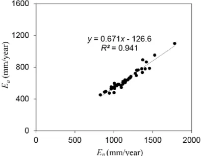
Monthly actual evaporation Ea was converted from monthly potential evaporation Ep
by multiplying Ep by the ratio of the number of sunny days in a month to the total number of days in a month. However, data pertaining to sunny days were only available from 1996–2014.
Therefore, the average monthly fraction of sunny days from 1996–2014 was used to extend Ea
over 1962–1995. After conducting this extension, we then investigated the correlation
between annual Ea and annual Ep for the entire period of 1962–2014. The strong correlation (R2=0.94) of Ea and Ep (Figure 3.4) indicated that extended Ea can be used as input data to calibrate the tank model in this study.
Figure 3.4. Correlation between annual Ep and annual Ea between 1962 and 2014 3.4.2. Change points of annual precipitation and discharge
To determine the turning points of the annual rainfall and discharge from 1962–2014, we used the cumulative anomaly test and the Pettit test. According to the Pettitt test results, there was no change-point year detected at p=0.05. However, change points of annual rainfall series were detected at p=0.48 in 1982. The annual discharge series at Quy Chau station was detected at p=0.21 in 1977. The annual discharge series at Nghia Khanh station was detected at p=0.64 in 1996.
In accordance with the Pettitt test results, the cumulative anomaly test results showed that the turning point of annual rainfall series occurred in 1982 (Figure 3.5a). The turning points of annual discharge series were in 1977 and 1997 at Quy Chau station (Figure 3.5b), and the turning points of annual discharge series were in 1977 and 1996 at Nghia Khanh station (Figure 3.5c).
At the breaking point of 1982, the mean annual rainfall decreased from 1767 mm from 1962–1982 to 1602 mm from 1983–2014 (Figure 3.6a). However, the discharge series increased after 1977 and then subsequently decreased after 1997 at both stations (Figure 3.6b&c).
(a) (b)
(c)
Figure 3.5. Cumulative anomaly test results of annual rainfall (a), annual discharge at Quy Chau station (b) and annual discharge at Nghia Khanh station (c)
(a) (b)
(c)
Figure 3.6. Mean annual rainfall (a), mean annual discharge at Quy Chau station (b) and mean annual discharge at Nghia Khanh station (c); break points are identified 3.4.3. Trial of tank model calibration for the whole period of 1962–2014
Prior verification of the annual water balance was conducted for the long-term analyses before calibrating the tank model. In a catchment, the water input and the output must be balanced. However, in the research area, there was only a single meteorological station used for the input data. Therefore, the precipitation might not be representative of the entire catchment. This research assumes that monthly precipitation multiplied by the precipitation factors approximates the annual water balance. In addition, in order to simplify the tank model calibration, the actual evaporation was assumed to be accurate for this study.
Consequently, the annual water balance can be expressed as P × CP = Q + Ea, where CP is a precipitation factor (Sugawara et al. 1995).
At the Quy Chau hydrological station, the precipitation factor was 1.13 for 1962–2014.
At the Nghia Khanh hydrological station, CP was close to unity for 1973–2014. We used adjusted precipitation (P × CP), actual evaporation (Ea) and discharge (Q) to calibrate the tank model.
The calibration results of the tank model show that the base flow of the calculated discharge was consistently smaller than that of the observed discharge for 1984–1998 at both stations (Figure 3.7). Breaking points of the base flow were close to breaking points of precipitation and discharge detected by the cumulative anomaly test and the Pettitt test.
(a)
(b)
Figure 3.7. Calibrated tank model (a) at Quy Chau hydrological station for 1962–2014 and (b) at Nghia Khanh hydrological station for 1973–2014
3.4.4. Tank model calibration for the first period (1962–1983) at Quy Chau station
The study was divided into three time periods for additional study: pre-1984 (period 1), 1984–1998 (period 2) and post-1998 (period 3). We first simulated the tank model for period 1 and then applied the simulated parameters for periods 2 and 3. The value of the precipitation factor during each period was estimated using the annual water balance equation of Pi × CPi = Qi + Eai, where CPi is a precipitation factor during each period and i = 1, 2, 3 denotes the first, second and third periods, respectively. At Quy Chau, the results of CPi were 1.01 for the first period, 1.38 for the second period and 1.10 for the third period. At Nghia Khanh, the corresponding CPi values were 0.92, 1.08 and 0.96, respectively. The relative change in precipitation was calculated as (CPi–1)×100%. We found a significant lack of precipitation, with 38% at Quy Chau and 8% at Nghia Khanh during period 2.
The rainfall data at Quy Chau station were appropriate for catchment representation for periods 1 and 3, however insufficient to meet the water budget for period 2. Adjusting the precipitation by multiplying by a precipitation factor is apparently a simple method used for long-term analyses. However, the precipitation factor also shows a seasonal change (Sugawara et al., 1995). Therefore, using a precipitation factor that varies by month might yield better calibration results. In this case, the precipitation factor is described as CP(M), where M is the month index (Sugawara et al. 1995). In this study, CP(M) was calibrated by the number of trials.
The tank model was calibrated for period 1 (1962–1983) corresponding to two trials.
(1) Trial No. 1: Precipitation adjusted by multiplying by a constant precipitation factor.
However, CP at Quy Chau during 1962–1983 was close to 1.0. Therefore, the precipitation did not change.
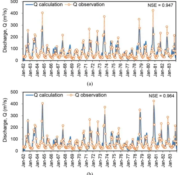
(2) Trial No. 2: Precipitation was adjusted by precipitation factor CP(M) (Sugawara et al., 1995). The available precipitation data were adjusted taking into consideration a high peak discharge. After the trials, the appropriate values of CP(M) were changed corresponding to different range of discharge. When the monthly discharge exceeded 400 m3/s, the precipitation was multiplied by CP(M)=1.5. If the monthly discharge was between 200 and 400 m3/s, the precipitation was multiplied by CP(M)=1.2. If the monthly discharge was less than 38 m3/s, the precipitation was not changed. The precipitation factor for the other months was 1.0.
In Figure 3.8, we show the results of tank model calibration for the two trials at Quy Chau station. The NSE and the coefficientof determination (R2) of trial No. 1 are 0.947 and
3.9 shows the improvement in trial No. 2 (b) compared with trial No. 1 (a) based on the better fit of the duration curve.
(a)
(b)
Figure 3.8. Calibrated tank model at the Quy Chau gauging station from 1962–1983 trial No. 1 and (b) trial No. 2
3.4.5. Tank model calibration for the first period (1973–1983) at Nghia Khanh station The tank model calibrated for 1973–1983 at Nghia Khanh made use of the same method as that applied to Quy Chau station. The appropriate values of CP(M) must be changed to correspond to a different range of monthly discharges. When the monthly discharge exceeds 400 m3/s, the precipitation is modified by multiplying it by CP(M)=1.4. If the monthly discharge is less than 64 m3/s, the precipitation was left unchanged. The precipitation factor for the remaining months was 0.92.
(a)
(b)
Figure 3.9. Duration curves at Quy Chau station from 1962–1983 (a) trial No. 1 and (b) trial No. 2
The results of the tank model calibration of the two trials at Nghia Khanh station are shown in Figure 3.10. The NSE and R2 values of trial No. 1 were 0.894 and 0.821, respectively. The corresponding values for trial No. 2 were 0.937 and 0.905, respectively. An improvement in calibration was noted for trial No. 2 compared with trial No. 1 (Figure 3.11).
These results indicate that a precipitation factor that varies with the month is useful for obtaining better calibration results. A month that has higher precipitation (discharge) necessitates a higher precipitation factor, which means that rainfall density might lead to a change in the relation between rainfall and infiltration, as well as surface runoff in the watershed (Basri 2013).
3.4.6. Tank model validation
The calibrated parameters in Figure 3.12 were applied to periods 2 and 3. A similar CP(M) was applied for periods 2 and 3 as for period 1 (trial No. 2). The model evaluation statistics for different periods are listed in Table 3.1. Our results indicate that the tank model applied for period 3 had better results of the NSE and R2 values than for period 2 at both
period 2. The results of the NSE and R2 values for periods 2 and 3 in this study were in line with the findings of Giang et al. (2014) (Table 3.1). These authors applied the SWAT model to the Upper Ca River. They found that, compared with the calibration period (1971–1995), the simulated discharge during the validation period (1996–2010) more closely followed the corresponding observed discharge; it underestimated the peak-flow months less and overestimated the low-flow months less.
(a)
(b)
Figure 3.10. Calibrated tank model at Nghia Khanh station from 1973–1983 (a) trial No. 1 and (b) trial No. 2
(a)
(b)
Figure 3.11. Duration curves at Nghia Khanh station from 1973–1983 (a) trial No. 1 and (b) trial No. 2
Table 3.1. Nash-Sutcliffe efficiency (NSE) and the coefficient of determination (R2) resultsfor different time periods
Stations Quy Chau (1960 km2)
Nghia Khanh (4024 km2)
Yen Thuong (23,000 km2) (Giang et al. 2014) Periods 1984–1998 1999–2014 1984–1998 1999–2014 1971–1995 1996–2010
NSE 0.895 0.920 0.892 0.896 0.86 0.89
R2 0.665 0.830 0.762 0.815 0.87 0.89
3.5. DISCUSSION
3.5.1. Tank model calibration using monthly input data
The tank model was calibrated for period 1 at the Upper Hieu River using the three- tank structure (Figure 3.2). However, the side outlet and infiltration coefficients for the third tank had very little effect on the simulation results. Therefore, the tank model composed of two tanks using monthly data was the most appropriate for simulating the Upper Hieu River
s
Figure 3.12. Calibrated parameters of the tank model using monthly data
Previous researchers have investigated the most appropriate number of tanks for the tank model. For example, Kuok et al. (2011) investigated three-tank, four-tank and five-tank models to ascertain the most appropriate tank model configuration for the southern region of Sarawak in Malaysia. These authors revealed that the four-tank model yielded the best runoff forecasting result. Kadarisman(1993) applied the tank model for the Babak River Basin, Lombok Island, Indonesia and concluded that the tank model with three tank components was unsuitable for use in low-flow analysis. The tank model with three tank components can be used for normal and high-accuracy analysis in cases in which the low flows are not significant.
Basri (2013) used the tank model with various types of land as a reference to determine the preferred number of tanks. This author advised using tank models of different types based on land use (e.g., four tanks for a forest, three tanks for a garden or vacant lot, two tanks for a paddy and one tank for a settlement). The number of tanks therefore depends on the catchment area. Pradhan (2001) reported that the numbers of tanks necessary for the tank model increases for larger-scale catchments to ensure better performance of the model. In nearly all earlier studies, daily data were used to calibrate the tank model (Kuok et al. 2011;
Mondal et al.2009; Pradhan 2001). In this study, monthly data were used as the input for the tank model. We found that a two-tank model with monthly input data was the most appropriate tank model for the Upper Hieu River.
3.5.2. Temporal change of runoff at the Upper Hieu River
The temporal change in runoff upstream of the Hieu River Basin was investigated for three time periods: prior to 1984, 1984–1998 and after 1998. Figures 3.13 shows the results of double mass curves of precipitation-calculated discharge and precipitation-observed discharge.
These data indicate that the increment of observed discharge was less than the increment of calculated discharge during period 3. The annual loss in discharge was 0.2×10⁹ m3 at Quy
Chau and 1.5×10⁹ m3 at Nghia Khanh between 1999 and 2014. This finding means the rate of discharge loss in the Lower Basin (between Quy Chau and Nghia Khanh) was approximately six times higher than that in the Upper Basin (upstream of Quy Chau).
(a)
(b)
Figure 3.13. Double mass curves of precipitation and discharge (a) Quy Chau and (b) Nghia Khanh
It has been reported that the annual runoff of many rivers around the world has decreased remarkably during recent decades (Shiklomanov 1993). The decrease in precipitation and/or the increase in evapotranspiration are considered to be factors that directly influence runoff decrease (Wang et al. 2012). The decrease in runoff might also result from anthropogenic influences in the catchment (e.g. population growth, river regulation, dam construction, irrigation) (Vörösmarty et al.2000; Yao et al. 2015). At the research site, the actual evaporation that we found also exhibited an increasing trend for the last 53 years, which resulted in reduction in runoff. In addition, many reservoirs have been constructed and
operated at upper Quy Chau since 2005 (e.g., Ban Kok, Sao Va and Nhan Hac, which have electricity generation capacities of 18, 3, and 45 MW, respectively). There are two major reservoirs between Quy Chau and Nghia Khanh: Sao-River reservoir and Ban Mong reservoir.
Construction of the Sao River reservoir, with a gross capacity of 5.1×10⁷ m3, started at the end of 1999 and finished in 2003. It was designed to provide irrigation water for 6200 ha of land for rice cultivation, commercial crops and water reserves. Ban Mong reservoir, with a gross capacity of 2.5×10⁸ m3 and a power generation capacity of 42 MW, was first started in 2010 and ultimately completed in 2012. The reservoirs provide power generation, and water supply for residential and farming areas in the region. Moreover, they reduce flooding of the Hieu River downstream. All of the water used for agricultural and residential purposes, in addition to the water stored in the reservoirs, resulted in a marked decrease in the river runoff in the Hieu River Basin beginning in 1998, particularly at Nghia Khanh. In addition, the reservoir might engender increased potential evaporation and leakage losses, resulting in decreased runoff (Gao et al. 2011).
3.6. CONCLUSIONS
We have used a tank model calibrated with monthly input data to assess the temporal variation in river flow at the Upper Hieu River Basin in Vietnam during the time period 1962–2014. With cumulative anomaly tests and Pettitt tests, we detected turning points in annual rainfall and discharge. Our results reveal turning points in annual rainfall series in 1982 and turning points in the annual discharge series in 1977 and 1997 at Quy Chau. At Nghia Khanh, we noted turning points in the annual discharge series in 1977 and 1996. In addition, we calibrated the tank model at both stations for the 53 years of observations. The base flow of the calculated discharge was less than that of the observed result from 1984–
1998. We assessed the flow variation for three time periods: 1962–1983 (period 1), 1984–
1998 (period 2) and 1999–2014 (period 3).
The value of the precipitation factor during each period was estimated by checking the annual water balance. The tank model was simulated for period 1. Then, we applied the calibrated parameters to periods 2 and 3. The precipitation and evaporation used as input data for calibrating the tank model came from a single meteorological station model with a catchment area of 1960 km2 at Quy Chau and 4024 km2 at Nghia Khanh. The results of tank model calibration indicated that the hydrographs improved when we used a precipitation factor as a function of the month. In addition, our results confirmed that a two-tank model with monthly input data is the most appropriate tank model for the Upper Hieu River. We
used the set of calibrated parameters applied to periods 2 and 3 to ascertain the temporal variation in the flow on the Upper Hieu River. The temporal variation of river flow was investigated by comparing the increase in calculated and observed discharges with increases in precipitation. A marked decrease in runoff has occurred since 1999, particularly at Nghia Khanh station. The rate of discharge loss in the Lower Basin was approximately six times higher than that in the Upper Basin, a finding likely due to reservoir construction and water being intensively used for agricultural and residential purpose.
REFERENCES
Basri H (2013) Development of rainfall-runoff model using tank model: Problems and challenges in province of Aceh, Indonesia. Aceh Int J Sci Technol 2(1): 26–36
Chikamori H, Heng L, Daniel T (eds) (2012) Catalogue of rivers for Southeast Asia and the Pacific – Volume VI. UNESCO-IHP Regional Steering Committee for Southeast Asia and the Pacific
Cung NV (ed) (1979) Technical Manual for Irrigation. The Agricultural Publishing House, Ha Noi. (In Vietnamese)
ENV–Vietnam Electricity (2001) Feasibility study for Ban La hydropower project, meteorological condition. Ha Noi, Vietnam. (In Vietnamese)
Gao P, Mu X-M, Wang F, Li R (2011) Changes in streamflow and sediment discharge and the response to human activities in the middle reaches of the Yellow River. Hydrol Earth Syst Sci 15: 1–10
Giang PQ, Toshiki K, Sakata M, Kunikane S, Vinh TQ (2014) Modelling climate change impacts on the seasonality of water resources in the upper Ca river watershed in Southeast Asia. Sci World J
Kadarisman (1993) A comparative study of the application of two catchment models to the Babak River Basin Lombok Island – Indonesia. Memorial University of Newfoundland.
Retrieved from http://research.library.mun.ca/id/eprint/5308
Kuok K, Harun S, Chiu P-C (2011) Investigation best number of tanks for hydrological tank model for rural catchment in humid region. J Inst Eng, Malays 72(4): 1–11
Liu C, Zheng H (2002) Hydrological cycle changes in China`s large river basin: The Yellow River drained dry. In M. Beniston (ed), Climatic Change: Implications for the Hydrological Cycle and for Water Management (pp. 209–224). Kluwer, Dordrecht
Mondal MS, Kouchi Y, Okubo K (2009) Sedimentation and thermal stratification during floods: A case study on Hail Haor of North-East Bangladesh. J Hydrol Meteorol 6(1):
15–25
Nyadawa MO, Kobatake S, Ezaki K (1996) A modified tank model and applications in some river basins in Kenya. Jpn Soc Hydrol Water Res 9(6): 498–512. Retrieved from https://www.jstage.jst.go.jp/article/jjshwr1988/9/6/9_6_498/_article
Pradhan NR (2001) Applicability of BTOPMC model and tank model in sub-catchments of Sun Kosi Basin, Nepal. Tribhuvan University
Shiklomanov I (1993) World fresh water resources. In P. H. Gleick (ed), Water in crisis a guide to the world’s fresh water resources (pp. 13–24). Oxford University Press, New York
Sugawara M (1995) Chapter 6: Tank model. In V. P. Singh (ed), Computer models of watershed hydrology (pp. 165–214). Water Resources Publications, Highlands Ranch, Colorado
Vörösmarty CJ, Green P, Salisbury J, Lammers RB (2000) Global water resources:
vulnerability from climate change and population growth. Science 289(5477): 284–288 Wang S, Yan M, Yan Y, Shi C, He L (2012) Contributions of climate change and human
activities to the changes in runoff increment in different sections of the Yellow River.
Quat Int 282: 66–77
Yao H, Shi C, Shao W, Bai J, Yang H (2015) Impacts of climate change and human activities on runoff and sediment load of the Xiliugou Basin in the Upper Yellow River. Adv Meteorol
Zhang L, Dawes WR, Walker GR (2001) Response of mean annual evapotranspiration to vegetation changes at catchment scale. Water Res 37(3): 701–708