XufengZhaoPh.D.dissertation,February2013 StudiesonExtendedCumulativeDamageModelsandTheirApplicationstoGarbageCollections BusinessAdministrationAichiInstituteofTechnologyToyota,Japan

(1)

Business Administration

Studies on Extended Cumulative Damage Models and Their Applications to Garbage Collections

Xufeng Zhao

Ph.D. dissertation, February 2013

(2)

(3)

Business Administration

Studies on Extended Cumulative Damage Models and Their Applications to Garbage Collections

Xufeng Zhao

Ph.D. dissertation, February 2013

(4)

(5)

Studies on Extended Cumulative Damage Models and Their Applications to Garbage Collections

Prepared by: Xufeng Zhao

Supervisor: Professor Toshio Nakagawa

Release date: February 2013 Category: Public

Edition: Final version

Keywords: Reliability, maintenance, damage model, garbage collection Comments: This dissertation is submitted in partial fulfillment for the

degree of Doctor of Philosophy at Aichi Institute of Tech- nology

Department of Business Administration Aichi Institute of Technology

Toyota, 470-0392, Japan

http://www.ait.ac.jp/index.html Tel: (+81) 565-48-8121

(6)

(7)

Abstract

This dissertation proposes several maintenance policies for extended cumulative damage models in reliability theory and their applications to garbage collection policies for a generational garbage collector in computer science. Using the techniques of cumulative processes, the expected costs per unit of time, i.e., expected cost rate models, are obtained, and optimal policies which minimize them are discussed analytically and computed numerically.

An initial chapter gives introduction which is constructed by review of literatures and organization of dissertation. Extended cumulative damage models in theory and their optimizations are proposed in the following chapters: Chapter 2 proposes two basic preventive maintenance policies for a used system with an initial variable damage level. Chapter 3 considers three replacement policies that are combined additive with independent damages. Chapter 4 takes up three maintenance policies for an operating system which works at random times for jobs. Chapter 5 proposes a standard cumulative damage model in which the notion of “whichever occurs last” is applied, which is called maintenance last. As applications, two stochastic models based on the working schemes of a generational garbage collector are proposed in Chapter 6. In the end of dissertation, the results are summarized and future problems are given.

The models proposed in Chapters 2–5 are derived from practical systems as introduced in every chapter and could be applied to them by suitable modifications and extensions. The theoretical methods proposed in Chapter 6 could provide some useful information to computer programmers to design more efficient collectors.

(8)

(9)

Acknowledgment

The author would like to appreciate Professor T. Nakagawa, the supervisor of my Ph.D. course, for his constant guidance, encouragement and suggestions through this dissertation.

The author wishes to thank the members of this dissertation reviewing com- mittee: Professor T. Kondo and Professor N. Ito of Aichi Institute of Technology.

The author is grateful to Professor S. Nakamura of Kinjo Gakuin University, Professor C. Qian of Nanjing University of Technology, Professor M. Chen of Fu Jen Catholic University, and Dr. S. Mizutani of Aichi University of Technology for their encouragement and cooperation during my Ph.D. course.

The author expresses thanks to Professor T. Dohi of Hiroshima University and Professor M. Kimura of Hosei University for having presented my related research at some international conferences, and is also grateful to Professor S. Sheu of Prov- idence University, Professor L. Cui of Beĳing Institute of Technology, Professor S.

Yamada of Tottori University, Professor Y. Hayakawa of Waseda University, Pro- fessor S. Chukova of Victoria University, and Professor M. J. Zuo of University of Alberta, who have helped me a lot in my research papers.

Furthermore, the author wishes to thank all members of Nagoya Computer and Reliability Research Group for their useful comments and discussions, and thank all members of Department of Business Administration, Aichi Institute of Technology, for their all kinds of help.

Finally, it is a special pleasure to thank my family for their mental and various supports.

(10)

(11)

List of Tables

2.1 Optimal λT^∗ and C(T^∗)/(λc_T) for c_K/c_T and z₀. . . 14

2.2 Optimal N^∗ and C(N^∗)/(λc_N)for c_K/c_N and z₀. . . 14

2.3 Optimal Tb^∗ and C(b Tb^∗)/c_T for c_M/c_T and c_K/c_T. . . 17

2.4 Optimal Nb^∗ and C(b Nb^∗)/cN for cM/cN and cK/cN. . . 17

3.1 Optimal T₁^∗ and C₁(T₁^∗)/c_T whenT₀ = 1, µ_T = 1 and K = 20. . . . 31

3.2 Optimal N₂^∗ and C₂(N₂^∗)/c_N when T₀ = 1,µ_T = 1 and K = 20. . . . 32

3.3 Optimal T₃^∗ and C₃(T₃^∗)/c_T whenT₀ = 1, µ_T = 1 and K = 20. . . . 32

3.4 Optimal N₄^∗ and C₄(N₄^∗)/c_N when T₀ = 1,µ_T = 1 and K = 20. . . . 33

3.5 Optimal T₅^∗ and C₅(T₅^∗)/c_T whenT₀ = 1, µ_T = 1 and K = 20. . . . 33

4.1 Optimal N₁^∗ and C₁(N₁^∗)/(λc_N) for µK and c_K/c_N. . . 40

4.2 Optimal N₂^∗ and C₂(N₂^∗)/(λc_M) for G^∗(β)and c_N/c_M. . . 42

4.3 Optimal Ne₂^∗ and Ce₂(Ne₂^∗)/(λc_M) for µK and c_N/c_M. . . 42

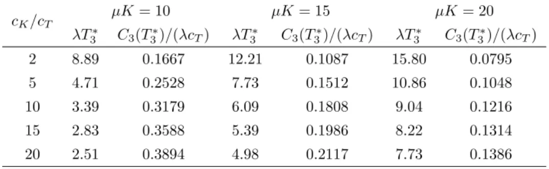
4.4 Optimal λT₃^∗ and C3(T₃^∗)/(λcT) forµK and cK/cT. . . 45

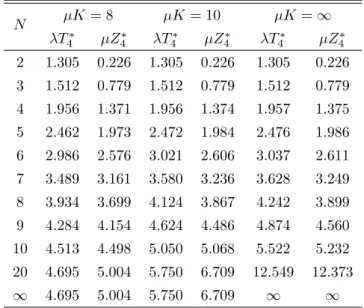
4.5 Optimal λT₄^∗ and µZ₄^∗ for µK and N. . . 52

5.1 Optimal T_L^∗, T_F^∗, and their cost rates when λ= 1, µ= 1, K = 10. . 64

5.2 Optimal Z_L^∗, Z_F^∗, and their cost rates when λ= 1,µ= 1, K = 10. . 68

5.3 Optimal N_L^∗, N_F^∗, and their cost rates when λ= 1,µ= 1, K = 10. . 73

6.1 Optimal λT₁^∗ and C₁(T₁^∗)/λ whenc_S = 10, c_M = 1 and σ = 1. . . . 89

6.2 Optimal K₁^∗ and C₁(K₁^∗)/λ when c_S = 10, c_M = 1 and σ = 1. . . 90

(16)

6.3 Optimal λT₂^∗ and C₂(T₂^∗)/λ for α and β. . . 99

6.4 Optimal N₂^∗ and C₂(N₂^∗)/λ for α and β. . . 100

6.5 Optimal λT₃^∗ and C3(T₃^∗)/λ for α and β. . . 101

6.6 Optimal N₃^∗ and C₃(N₃^∗)/λ for α and β. . . 101

(17)

List of Figures

6.1 Working schemes of a generational garbage collector. . . 82 6.2 Major collection including minor and tenuring collections. . . 91 6.3 Major collection including tenuring collections. . . 95

(18)

(19)

Chapter 1

Introduction

1.1 Review of Literatures

Public infrastructures in advanced nations are now becoming obsolete (Hudson, et al., 1997), and the number of aged plants in Japan is increasing greatly in the near future (Nakagawa and Ito, 2008). A deliberate maintenance plan is indispensable to operate such systems without serious trouble caused by failures. That is, systems should undergo suitable maintenances at adequate times by considering both profits of operations and losses of unexpected failures or maintenances (Zhao, et al., 2012a).

We call that maintenances after failure and before failure are corrective maintenance (CM) and preventive maintenance (PM), respectively (Nakagawa, 2005, p.2). CM may be costly, and sometimes requires a long time, so that how to determine the schedule of PM becomes an important problem for an operating system. However, it is not wise to maintain a system with unnecessary frequency.

A methodical survery of maintenance policies in reliability theory was done (Nakagawa, 2005). The recent published books (Osaki, 2002; Wang and Pham, 2007; Kobbacy and Murthy, 2008; Nakagawa, 2008, 2011; Manzini, et al., 2010) collected many maintenance models in theory and their applications in industrial systems. On the other hand, most systems might fail due to the damage stored within them by shocks such as jolt, stress, or environment change. This is well-

(20)

1.1. Review of Literatures

known as the cumulative damage model (Cox, 1962) which plays an important role in reliability theory: The model is considered as a sequence of shocks which occur randomly in time as an event in accordance with a stochastic process and give some amount of damage to a system. The damage suffered for the system is accumulated to the current damage level and weakens the system gradually. The system fails when the total damage exceeds a failure level.

Some reliability quantities of cumulative damage models have already been obtained (Cox, 1962; Esary, et al., 1973; Nakagawa and Osaki, 1974). The first research book (Bogdanoff and Kozin, 1985) introduced some probabilistic models which are related to cumulative damage, however, the case studies for the models are few and the analyses might be too difficult theoretically to apply them to practical models. To build a bridge between theory and practice, book (Nakagawa, 2007) summarized sufficiently PM policies and their optimization problems for shock and damage models, using the techniques of stochastic processes. A variety of PM models subjected to shocks were studied extensively (Wortman, et al., 1994; Sheu, et al., 1996, 1998, 2002, 2004, 2012; Qian, et al., 2005; Zhao, et al., 2010a, 2011a, 2012a, 2012b). The damage models have been applied to garbage collection models (Satow, et al., 1996a, 1196b) by replacing shock by update and damage by garbage, backup models of database systems (Qian, et al., 1999, 2002a, 2002b, 2010; Naka- mura, et al., 2003) by replacing shock by update and damage by dumped file, and software rejuvenation models (Zhao, et al., 2009) in computer sciences by replacing shock by aging-related fault and damage by consumption of physical memory.

In the computer science community, the technique of garbage collection (Jones and Lins, 1996) is one automatic process of memory recycling, which refers to that objects in the memory no longer referenced by programs are called garbage and should be thrown away. A garbage collector determines which objects are garbage and makes the heap space occupied by such garbage available again for the subsequent new objects. Garbage collection plays an important role in Java’s security strategy, however, it adds a large overhead that can deteriorate the program performances. From related studies which are summarized in (Jones and Lins, 1996), a garbage collector spends between 25 and 40 percent of execution time of programs for its work in general, and delays caused by such a garbage collection

(21)

1.2. Organization of Dissertation are obtrusive.

With regarding to garbage collection modeling and optimization, there have been very few research papers that studied analytical expressions of optimal policies for a garbage collector. The modeling methods (Satow, et al., 1996a, 1196b) did not consider the theoretical point of garbage collection working schemes essentially.

Most problems in other literatures were concerned with several ways to introduce garbage collection methods in techniques and how to tune the garbage collector by simulations, which is more complex and time consuming due to the random accesses of programs in the memory in practice (Ungar and Jackson, 1992; Kaldewaĳ and Vries, 2001; Lee and Chang, 2004; Clinger and Rojas, 2006; Soman and Krintz, 2007). We propose that garbage collection is a stochastic decision making process and should be analyzed by the theory of stochastic processes from the viewpoints of management. Optimal policies for a generational garbage collector with tenuring threshold and major collection times according to practical working schemes (Zhao, et al., 2010b, 2011b, 2012c) were studied recently.

1.2 Organization of Dissertation

The main body of this dissertation is divided into Introduction, Chapters 2–6, Conclusions, and Bibliography.

Chapter 2 gives a definition of a used system with an initial variable damage level Y₀, and proposes two basic imperfect PM policies which are done at a planned timeT or at a shock numberN. Furthermore, two extended models, by considering increasing inspection costs suffered for shocks, are formulated.

Chapter 3 proposes that the system would fail by both additive and independent damages, and considers three replacement policies with such two kinds of damages: The unit is replaced at a planned time and undergoes minimal repair when independent damage occurs. First, a standard cumulative damage model where the unit is replaced at a planned time T is considered. Second, the total damage is measured only at periodic times nT₀. Third, the total damage increases linearly with time t approximately.

Chapter 4 takes up three maintenance policies for an operating system which

(22)

1.2. Organization of Dissertation

works at random times for jobs. First, PM is made at the Nth completion of working time, and the system fails with probability p(x) when the total damage is x. Second, the system is maintained at the first completion of some working times over timeT. Third, when a limit number N of working times are considered, maintenance is made at a planned time T or at a damage level Z.

Chapter 5 gives two definitions of maintenance first (MF) and maintenance last (ML), where MF has been discussed widely in literatures, and MF denotes that PM is done before failure at a planned time T, at a damage level Z, or at a shock number N, whichever occurs last. To derive the optimization problems, two alternative policies which combined time-based with condition-based PM are discussed, i.e., optimal policies of T_L^∗ for N, Z_L^∗ for T, and N_L^∗ for T are obtained.

Comparison methods between such a ML and the conventional MF are explored.

Chapter 6 proposes two application models of cumulative damage processes to garbage collection policies in computer science, according to the practical working schemes of a generational garbage collector. We suppose that garbage collections occur at a nonhomogeneous Poisson process, and divide the collections into minor, tenuring, and major collections, respectively. Minor collections are made when the garbage collector begins to work, tenuring collection is made at a planned time T or at the first collection time when surviving objects have exceeded K, and major collection is made at time T or at the Nth collection.

In Chapters 2–6, expected cost rates for all policies are obtained, by using the techniques of cumulative processes in reliability theory. Optimal policies are discussed analytically, and numerical examples are computed when a Poisson process and exponential or normal distributions are adopted. The models proposed in Chapters 2–5 can also be applied to practical systems: Chapter 2 could be modified in garbage collection or defragmentation models in software systems when collection or defragment is imperfect. Chapter 3 could be used in reorganization models of a structural database. When the operating system is executing jobs or computer procedures successively, Chapters 4 and 5 could provide new topics and methods as practical policies.

Finally, chapter 7 summaries the results that have been obtained in this dissertation.

(23)

Chapter 2

Maintenance for a Used System

In some practical situations, it may be more economical to operate a used system than to do a new one. From this viewpoint, this chapter proposes two basic preventive maintenance policies for a used system: The system with an initial variable damage Y₀ begins to operate at time 0, and suffers damage due to shocks. It fails when the total damage exceeds a failure levelK and corrective maintenance is made immediately. To prevent such a failure, it undergoes preventive maintenance at a planned time T or at a shock numberN, but maintenances are imperfect. Further- more, increasing inspection cost that is suffered for every shock is applied to the above policies in the extended models. Using the theory of cumulative processes in reliability, expected cost rate models are obtained, and optimal policies which minimize them are derived analytically and discussed numerically.

2.1 Introduction

As introduced in Chapter 1, maintenances after failure and before failure are called corrective maintenance (CM) and preventive maintenance (PM), respectively. When CM is done, it may require much more time and higher cost, so we need to do PM to prevent failure. Even so, we should not to do it too often from the viewpoints of time and cost. In this case, various PM policies and their optimizations, which

(24)

2.2. Expected Cost Rate

make the system as good as new, including some minimal repairs, were summarized in (Nakagawa, 2005). However, CM and PM would not make a system like new but younger, i.e., maintenances are imperfect in general. Some imperfect PM models have been considered in (Chan and Downs, 1978; Murthy and Nguyen, 1981; Brown and Proschan, 1983; Wang and Pham, 2003; Nakagawa, 2005, 2007). In some practical situations, it may be more economical to operate a used system than to do a new one. Optimal replacement policies for a used system were studied in (Muth, 1977; Nakagawa, 1979; Qian, et al., 2005). However, an initial damage level of the system at time 0 or after imperfect PM may be a variable and its distribution function may be different from those of damage caused by shocks during its operation.

We suppose that a used system begins to operate at time 0, and its initial damage is a random variable Y₀ (0≤Y₀ ≤K). Shocks occur at a nonhomogeneous Poisson process and each shock causes a random amount of damage to the system.

These damages are accumulated to the current damage level. The system undergoes imperfect preventive maintenance (IPM) at a planned time T (0 < T ≤ ∞), at a shock number N (N = 1,2,· · ·), or imperfect corrective maintenance (ICM) is done when the total damage exceeds a failure level K, whichever occurs first. The expected cost rates are obtained by using the techniques of cumulative damage models (Nakagawa, 2007), and optimal maintenance policies which minimize them are discussed analytically. Furthermore, increasing inspection cost that is suffered for every shock is applied to the above policies in extended models, the expected cost rates are obtained and computed numerically.

2.2 Expected Cost Rate

Suppose that shocks occur at a nonhomogeneous Poisson process with an intensity functionλ(t)and a mean-value functionR(t)≡Rt

0 λ(u)du, i.e.,λ(t)≡R⁰(t). Then, the probability that shocks occur exactlyj times in the interval [0, t]is (Nakagawa, 2007, p.21)

H_j(t)≡ [R(t)]^j

j! e^−R(t) (j = 0,1,2,· · ·).

(25)

2.2. Expected Cost Rate It is assumed that the system with an initial damage Y0 begins to operate at time 0, where Y₀ is a random variable and has a distribution function G₀(x) = Pr{Y₀ ≤x}forx≤K andG₀(x)≡1forx > K with meanµ₀ ≡RK

0 G₀(x)dx < K, i.e., RK

0 G₀(x)dx=K−µ₀. Further, an amountY_j of damage due to thejth shock has an distribution function G(y) ≡Pr{Y_j ≤ y} (j = 1,2,· · ·), these damages are accumulated to the current damage level. We call the system as a used system.

Then, the total damageZj ≡Y0+Pj

i=1Yi (j = 1,2,· · ·)up to thejth shock, where Z₀ ≡Y₀, has a distribution function

Pr{Z_j ≤w}= Z w

0

G^(j)(w−x)dG₀(x) (j = 0,1,2,· · ·), (2.1) where G^(j)(x) represents the j-fold Stieltjes convolution of G(x) with itself, and G⁽⁰⁾(x)≡1for x≥0.

LetZ(t)be the total damage at timet. Then, the distribution function ofZ(t) is

Pr{Z(t)≤w}=

∞

X

j=0

H_j(t) Z w

0

G^(j)(w−x)dG₀(x). (2.2)

Suppose that the system undergoes ICM when the total damage exceeds a failure level K, and undergoes IPM at a planned timeT (0< T ≤ ∞)or at a shock number N (N = 1,2,· · ·), whichever occurs first. The damage level decreases to Y₀ by either IPM or ICM, i.e., the system becomes an identical system with an initial damage level Y₀ which has a general distribution G₀(x). However, the cost for ICM would be higher than that for IPM, because the system might suffer serious damage when the total damage has exceeded a failure levelK. Furthermore, the maintenance cost might be affected by the amount of total damage when the system undergoes ICM and IPM. From the above reasons, we introduce the following maintenance costs: Cost c_T and c_N are the respected fixed costs for IPM at time T and at shock N, and c_K is the fixed cost for ICM, where c_T < c_K and c_N < c_K. In addition, c₀(x) (0≤x≤K) is an additional cost when the total damage isx at maintenance time.

For the above system, the probability that the system undergoes IPM at time

(26)

2.2. Expected Cost Rate T is

P_T =

N−1

X

j=0

H_j(T) Z K

0

G^(j)(K−x)dG₀(x), (2.3) and the probability that it undergoes IPM at shock N is

PN = Z T

0

HN−1(t)λ(t)dt Z K

0

G^(N)(K−x)dG0(x). (2.4) Thus, the expected cost when IPM is done is

C_{IP M} =

N−1

X

j=0

H_j(T) Z K

0

Z K−x 0

[c_T +c₀(x+y)]dG^(j)(y)dG₀(x) +

Z T 0

HN−1(t)λ(t)dt Z K

0

Z K−x 0

[c_N +c₀(x+y)]dG^(j)(y)dG₀(x). (2.5) The probability that the system undergoes ICM when the total damage exceeds a failure levelK is

P_K =

N−1

X

j=0

Z T 0

H_j(t)λ(t)dt Z K

0

Z K−x 0

G(K −x−y)dG^(j)(y)dG₀(x), (2.6) whereΦ(x)≡1−Φ(x)for any function Φ(x), and the probability that the system undergoes ICM when the total damage exceeds K at shock N is included in (2.6) because it has become the failure state. Note that P_T + P_N + P_K ≡1. Thus, the expected cost when ICM is done is

C_ICM = [c_K+c₀(K)]

N−1

X

j=0

Z T 0

H_j(t)λ(t)dt Z K

0

Z K−x 0

G(K−x−y)dG^(j)(y)dG₀(x).

(2.7) The mean time to maintenance is

E(L) =T

N−1

X

j=0

H_j(T) Z K

0

G^(j)(K−x)dG₀(x) +

Z T

0

tH_N−1(t)λ(t)dt Z K

0

G^(N)(K−x)dG₀(x) +

N−1

X

j=0

Z T 0

tH_j(t)λ(t)dt Z K

0

Z K−x 0

G(K−x−y)dG^(j)(y)dG₀(x)

(27)

2.3. Optimal Policies

=

N−1

X

j=0

Z T 0

H_j(t)dt Z K

0

G^(j)(K−x)dG₀(x). (2.8)

Therefore, the expected cost rate is, from (2.5), (2.7), and (2.8),

C(T, N) =

c_K+c₀(K)−(c_K −c_T)PN−1

j=0 H_j(T)RK

0 G^(j)(K−x)dG₀(x)

−(cK −cN)RT

0 HN−1(t)λ(t)dtRK

0 G^(N⁾(K−x)dG0(x)

−PN−1

j=0 H_j(T)RK 0

RK

x G^(j)(u−x)dc₀(u)dG₀(x)

−RT

0 H_N−1(t)λ(t)dtRK 0

RK

x G^(N⁾(u−x)dc₀(u)dG₀(x) PN−1

j=0

RT

0 H_j(t)dtRK

0 G^(j)(K −x)dG₀(x) . (2.9)

2.3 Optimal Policies

2.3.1 Planned Time

Suppose that the system undergoes IPM only at time T (0 < T ≤ ∞) and ICM when the total damage exceeds a failure level K, whichever occurs first. Then, putting that N =∞ in (2.9), the expected cost rate is

C(T) =

c_K+c₀(K)−(c_K −c_T)P∞

j=0H_j(T)RK

0 G^(j)(K−x)dG₀(x)

−P∞

j=0H_j(T)RK 0

RK

x G^(j)(u−x)dc₀(u)dG₀(x) P∞

j=0

RT

0 H_j(t)dtRK

0 G^(j)(K−x)dG₀(x) . (2.10) We seek an optimal time T^∗ that minimizes C(T) in (2.10). Differentiating C(T) with respect toT and setting it equal to zero,

λ(T){(c_K−c_T)[1−Q(T)] +P(T)}

∞

X

j=0

Z T 0

H_j(t)dt Z K

0

G^(j)(K −x)dG₀(x) + (c_K−c_T)

∞

X

j=0

H_j(T) Z K

0

G^(j)(K −x)dG₀(x) +

∞

X

j=0

H_j(T) Z K

0

Z K x

G^(j)(u−x)dc₀(u)dG₀(x) =c_K+c₀(K), (2.11) where

P(T)≡ P∞

j=0Hj(T)RK 0

RK

x [G^(j)(u−x)−G^(j+1)(u−x)]dc0(u)dG0(x) P∞

j=0H_j(T)RK

0 G^(j)(K−x)dG₀(x) ,

(28)

Q(T)≡ P∞

j=0Hj(T)RK

0 G^(j+1)(K−x)dG0(x) P∞

j=0H_j(T)RK

0 G^(j)(K−x)dG₀(x) .

If there exists T^∗ which minimizes C(T), it must be satisfied (2.11).

It is assumed that shocks occur in a Poisson process with rate λ, the amount of damage due to each shock has an exponential distribution with mean µ, and c₀(x) is proportional to the total damage x, i.e., H_j(t) = [(λt)^j/j!]e^−λt, G^(j)(x) = P∞

i=j[(x/µ)ⁱ/i!]e^−x/µ, andc₀(x) =c₀x. Then,P(T) = c₀µQ(T), and (2.11) becomes λ[(c_K−c_T)−(c_K−c_T −c₀µ)Q₁(T)]

∞

X

j=0

Z T 0

H_j(t)dt Z K

0

G^(j)(K−x)dG₀(x) + (c_K−c_T)

∞

X

j=0

H_j(T) Z K

0

G^(j)(K −x)dG₀(x) +c₀

∞

X

j=0

H_j(T) Z K

0

Z K x

G^(j)(u−x)dudG₀(x) = c_K +c₀K. (2.12)

Denote the left-hand side in (2.12) beU(T), because RK

0 G₀(x)dx=K−µ₀, lim

T→0U₁(T) =c_K−c_T +c₀(K−µ₀)< c_K +c₀K, and M(x)≡P∞

j=1G^(j)(x) =x/µ and lim_T→∞Q(T) = 1,

Tlim→∞U(T) = (cK−cT) Z K

0

[1 +M(K−x)]dG0(x)

= (cK−cT)

1 + 1 µ

Z K 0

G0(x)dx

= (cK −cT)

1 + K −µ0

µ

. DifferentiatingU(T) with respect toT,

U⁰(T)

λ =−(c_K−c_T −c₀µ)Q⁰(T)

∞

X

j=0

Z T 0

H_j(t)dt Z K

0

G^(j)(K−x)dG₀(x).

Thus, if Q⁰(T) < 0 and c_K −c_T −c₀µ > 0, U(T) is a strictly increasing function of T, and hence, if a solution T^∗ to (2.12) exists, it is unique. It is clear that the necessity of optimal maintenance policy is that cost c_K for ICM should be greater thanc_T+c₀µfor IPM, which represents the total cost of a fixed cost for IPM and the maintenance cost for a mean initial damage. Note that 1−Q(T)means physically

(29)

2.3. Optimal Policies the probability of failure at the (j + 1)th (j = 0,1,2,· · ·) shock in time T, given that the system has not failed at the jth shock. Thus, the condition that a finite T^∗ satisfies (2.12) is that 1−Q(T) increases strictly, i.e., Q⁰(T)<0.

In particular, when Y₀ = z₀ (0 < z₀ < K), i.e., G₀(x) ≡ 1 for x ≥ z₀, 0 for x < z₀, it is proved thatQ⁰(T)<0. Thus, ifc_K−c_T > µ(c_T +c₀K)/(K−z₀), then there exists a finite and unique T^∗ (0 < T^∗ < ∞) which satisfies (2.12), and the resulting cost rate is

C(T^∗)

λ = (c_K −c_T)−(c_K −c_T −c₀µ)Q(T^∗). (2.13) Next, suppose thatG0(x) = (1−e^−x/z⁰)/(1−e^−K/z⁰) forx≤K, 1 for x > K, i.e., µ₀ = z₀ −Ke^−K/z⁰/(1−e^−K/z⁰). It can be proved from Appendix that Q(T) decreases strictly with T, and so that, U(T) increases strictly with T. Therefore, we have the following optimal policy:

1. If cK −cT > µ(cT +c0K)/(K −µ0) , then there exists a finite and unique T^∗ (0< T^∗ <∞)which satisfies (2.12), and the resulting cost rate is given in (2.13).

2. If c_K −c_T ≤µ(c_T +c₀K)/(K−µ₀), thenT^∗ =∞, and C(∞)

λ = c_K+c₀K

1 + (K−µ₀)/µ. (2.14)

2.3.2 Shock Number

Suppose that the system undergoes IPM only at shock N (N = 1,2,· · ·) and ICM when the total damage exceeds a failure level K, whichever occurs first. Then, putting that T =∞ in (2.9), the expected cost rate is

C(N) =

c_K+c₀(K)−(c_K −c_N)RK

0 G^(N)(K−x)dG₀(x)

−RK 0

RK

x G^(N⁾(u−x)dc₀(u)dG₀(x) PN−1

j=0

R∞

0 H_j(t)dtRK

0 G^(j)(K−x)dG₀(x) (N = 1,2,· · ·).

(2.15)

(30)

We seek an optimal number N^∗ that minimizes C(N) in (2.15). From the inequalityC(N + 1)−C(N)≥0,

{(c_K−c_N)[1−Q(N)] +P(N)}

PN−1 j=0

R∞

0 Hj(t)dtRK

0 G^(j)(K−x)dG0(x) R∞

0 H_N(t)dt + (c_K−c_N)

Z K 0

G^(N⁾(K−x)dG₀(x) +

Z K 0

Z K x

G^(N⁾(u−x)dc₀(u)dG₀(x)≥c_K+c₀(K), (2.16) where

P(N)≡ RK

0

RK

x [G^(N)(u−x)−G^(N+1)(u−x)]dc₀(u)dG₀(x) RK

0 G^(N⁾(K−x)dG₀(x) ,

Q(N)≡ RK

0 G^(N+1)(K−x)dG₀(x) RK

0 G^(N)(K−x)dG₀(x) .

If there exists N^∗ which minimizes C(N), it must be satisfied (2.16). It is clear that the necessity of optimal maintenance policy is that costc_K for ICM should be greater thanc_N+c₀µfor IPM. Note that1−Q(N)means physically the probability of failure at the (N + 1)th shock, given that the system has not failed at the Nth shock. Thus, the condition that a finiteN^∗ satisfies (2.16) is that1−Q(N)increases strictly.

The failure rate plays an important role of deriving analytically optimal policies for maintenance models (Nakagawa, 2005). The functions 1−Q(T) in (2.11) and 1−Q(N) in (2.16) correspond to the failure rates with continuous and discrete times, respectively, and would increase strictly when finiteT^∗ and N^∗ exist.

We make the similar assumptions in Section 2.3.1, thenP(N) =c₀µQ(N), and (2.16) becomes

[(cK−cN)−(cK−cN −c0µ)Q2(N)]

N−1

X

j=0

Z K 0

G^(j)(K−x)dG0(x) + (c_K−c_N)

Z K 0

G^(N⁾(K−x)dG₀(x) +c₀ Z K

0

Z K x

G^(N)(u−x)dudG₀(x)

≥c_K+c₀K. (2.17)

(31)

2.3. Optimal Policies Denote the left-hand side in (2.17) be U(N),

N→∞lim U(N) =(c_K−c_N) Z K

0

[1 +M(K−x)]dG₀(x)

=(c_K−c_N)

1 + K−µ₀ µ

,

U(N+ 1)−U(N) =−(c_K−c_N −c₀µ)[Q(N + 1)−Q(N)]

×

N−1

X

j=0

Z K 0

G^(j)(K −x)dG₀(x).

Thus, if Q(N) is a decreasing function of N and c_K −c_N −c₀µ > 0, U(N) is a increasing function of N, and hence, if a solution N^∗ to (2.17) exists, its minimum is unique.

In particular, when Y₀ = z₀ (0 < z₀ < K), i.e., G₀(x) ≡ 1 for x ≥ z₀, 0 for x < z₀, it is proved that Q(N) is a decreasing function of N. Thus, if c_K −c_N >

µ(c_N+c₀K)/(K−z₀), there exists a finite and unique minimumN^∗ (1≤N^∗ <∞) which satisfies (2.17), and the resulting cost rate is

(cK−cN −c0µ)Q(N^∗)≤(cK−cN)− C(N^∗)

λ <(cK −cN −c0µ)Q(N^∗−1).

(2.18) Next, suppose thatG₀(x) = (1−e^−x/z⁰)/(1−e^−K/z⁰) forx≤K, 1 for x > K.

It can be proved from Appendix that Q(N)decreases strictly with N, and so that, U(N) increases strictly withN. Therefore, we have the following optimal policy:

1. If c_K −c_N > µ(c_N +c₀K)/(K −µ₀) , then there exists a finite and unique minimumN^∗ (1≤N^∗ <∞)which satisfies (2.17), and the resulting cost rate is given in (2.18).

2. If c_K −c_N ≤ µ(c_N +c₀K)/(K −µ₀), then N^∗ = ∞, and the resulting cost rate is given in (2.14).

2.3.3 Numerical Examples

Suppose that G(x) = 1−e^−x/µ and G₀(x) = (1−e^−x/z⁰)/(1−e^−K/z⁰) for x≤ K.

We compute the optimal policies numerically when µ= 1, c0 = 0 and K = 20.

(32)

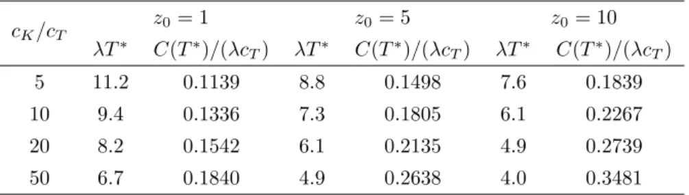
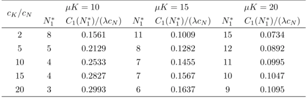
Table 2.1 presents optimal λT^∗ and C(T^∗)/(λcT) for cK/cT = 5, 10, 20, 50 and z₀ = 1, 5, 10. This indicates that T^∗ decreases when c_K/c_T or z₀ increases, C(T^∗) increases when c_K/c_T or z₀ increases. Table 2.2 presents optimal N^∗ and C(N^∗)/(λc_N) for c_K/c_N = 5, 10, 20, 50 and z₀ = 1, 5, 10. This shows the similar tendencies to Table 2.1 for N^∗ and C(N^∗). It is of interest that the order of the expected cost rates is C(T^∗)> C(N^∗) for the same value ofz₀ and c_T =c_N.

Table 2.1: Optimal λT^∗ andC(T^∗)/(λc_T)for c_K/c_T andz₀.

c_K/c_T z0= 1 z0= 5 z0= 10

λT^∗ C(T^∗)/(λcT) λT^∗ C(T^∗)/(λcT) λT^∗ C(T^∗)/(λcT)

5 11.2 0.1139 8.8 0.1498 7.6 0.1839

10 9.4 0.1336 7.3 0.1805 6.1 0.2267

20 8.2 0.1542 6.1 0.2135 4.9 0.2739

50 6.7 0.1840 4.9 0.2638 4.0 0.3481

Table 2.2: OptimalN^∗ andC(N^∗)/(λcN) for cK/cN andz0.

cK/cN

z₀= 1 z₀= 5 z₀= 10

N^∗ C(N^∗)/(λcN) N^∗ C(N^∗)/(λcN) N^∗ C(N^∗)/(λcN)

5 12 0.0952 10 0.1241 8 0.1510

10 11 0.1060 8 0.1405 7 0.1741

20 10 0.1169 7 0.1593 6 0.1981

50 9 0.1322 6 0.1843 5 0.2334

We could explain the optimal policies as follows: (1) When cost cK for ICM increases, we should advance the time of IPM, that is, T^∗ and N^∗ should be de- creased, in order to reduce the probability of failure. (2) When z₀ increases, i.e., a used system begins to operate at time 0 with a higher damage, then, its life will be shorter due to shocks, and so that,T^∗andN^∗ should be advanced. (3) Compare the numerical examples above, concrete performances of two policies would be depend on maintenance costs, system structures and environment, maintenance engineers,

(33)

2.4. Extended Models and so on. Take into such considerations, we would adopt which policy is suitable for an actual system. That is, from the viewpoint of economy, the policy N^∗ is better than that of T^∗. However, from the viewpoint of simplicity of operation, the policy T^∗ would be better because we do not need to count the number of shocks.

2.4 Extended Models

2.4.1 Expected Cost Rates

Introduce the cost c_{M i} suffered for the ith shock, where 0 < c_M₁ ≤ c_M₂ ≤ · · · ≤ c_{M i} ≤ · · ·. For example, this would be the inspection cost of measuring total damage level or the cost of some treatment for each shock, and would be usually much smaller compared to PM costs c_T and c_N.

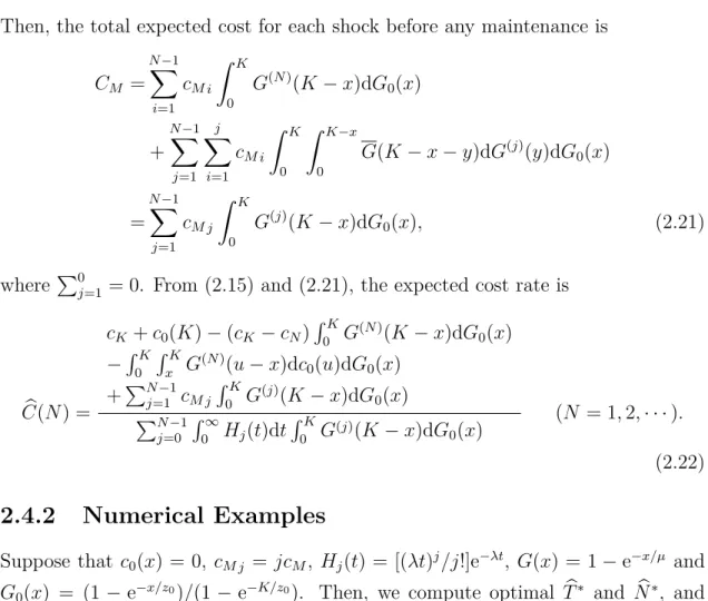
First, consider that the system undergoes IPM at time T (0 < T ≤ ∞) and ICM when the total damage exceeds a failure level K, whichever occurs first. Then, the total expected cost for each shock before any maintenance is

C_M =

∞

X

j=1 j

X

i=1

c_{M i}H_j(T) Z K

0

G^(j)(K−x)dG₀(x)

+

∞

X

j=1 j

X

i=1

cM i

Z T 0

Hj(t)λ(t)dt Z K

0

Z K−x 0

G(K−x−y)dG^(j)(y)dG0(x)

=

∞

X

j=0

c_{M j+1} Z T

0

H_j(t)λ(t)dt Z K

0

G^(j+1)(K −x)dG₀(x), (2.19)

From (2.10) and (2.19), the expected cost rate is

C(Tb ) =

c_K+c₀(K)−(c_K −c_T)P∞

j=0H_j(T)RK

0 G^(j)(K−x)dG₀(x)

−P∞

j=0H_j(T)RK 0

RK

x G^(j)(u−x)dc₀(u)dG₀(x) +P∞

j=0c_{M j+1}RT

0 H_j(t)λ(t)dtRK

0 G^(j+1)(K−x)dG₀(x) P∞

j=0

RT

0 Hj(t)dtRK

0 G^(j)(K−x)dG0(x) . (2.20) Second, consider that the system undergoes IPM at shock N (N = 1,2,· · ·) and ICM when the total damage exceeds a failure level K, whichever occurs first.

(34)

2.4. Extended Models

Then, the total expected cost for each shock before any maintenance is C_M =

N−1

X

i=1

c_{M i} Z K

0

G^(N)(K −x)dG₀(x)

+

N−1

X

j=1 j

X

i=1

c_{M i} Z K

0

Z K−x 0

G(K−x−y)dG^(j)(y)dG₀(x)

=

N−1

X

j=1

cM j

Z K 0

G^(j)(K −x)dG0(x), (2.21)

whereP0

j=1 = 0. From (2.15) and (2.21), the expected cost rate is

C(Nb ) =

c_K+c₀(K)−(c_K−c_N)RK

0 G^(N⁾(K−x)dG₀(x)

−RK 0

RK

x G^(N⁾(u−x)dc₀(u)dG₀(x) +PN−1

j=1 c_{M j}RK

0 G^(j)(K−x)dG₀(x) PN−1

j=0

R∞

0 Hj(t)dtRK

0 G^(j)(K−x)dG0(x) (N = 1,2,· · ·).

(2.22)

2.4.2 Numerical Examples

Suppose that c₀(x) = 0, c_{M j} = jc_M, H_j(t) = [(λt)^j/j!]e^−λt, G(x) = 1−e^−x/µ and G₀(x) = (1 −e^−x/z⁰)/(1−e^−K/z⁰). Then, we compute optimal Tb^∗ and Nb^∗, and C(b Tb^∗)/cT and C(b Nb^∗)/cN numerically when K = 20, z0 = 1, λ= 1,µ= 1.

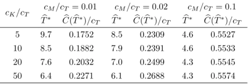
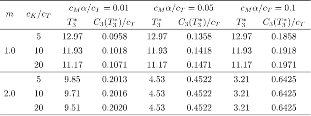
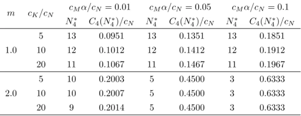
Table 2.3 presents optimal Tb^∗ and C(b Tb^∗)/c_T for c_M/c_T = 0.01, 0.02, 0.1 and c_K/c_T = 5, 10, 20, 50. This indicates that Tb^∗ decreases when c_K/c_T or c_M/c_T increases,C(b Tb^∗)increases whenc_K/c_T orc_M/c_T increases. Table 2.4 presents optimal Nb^∗ and C(b Nb^∗)/c_N for c_M/c_N = 0.01, 0.02, 0.1 and c_K/c_N = 5, 10, 20, 50. This shows the similar tendencies to Table 2.3 for Nb^∗ and C(b Nb^∗), but if c_M/c_N is very larger, whencK/cN increases, Nb^∗ andC(b Nb^∗)/cN will be stable. It is of interest that the order of the expected cost rates isC(b Tb^∗)>C(b Nb^∗)for the same parameters.

It could be explained as follows: (1) Compared with those in Section 2.3.3, optimal maintenance times are advanced due to shocks. (2) When costc_K for ICM increases, we should advance the time of IPM, the reason is the same as that in Section 2.3.3. (3) When c_M/c_T or c_M/c_N increases, it means unit cost for shocks will increase, so that IPM should be advanced to reduce the total expected cost for

(35)

2.5. Concluding Remarks shocks. (4) When the inspection cost for shocks is large, cost for ICM will have no effect on the optimal policies. It is interest of that for the two policies, both optimal policies and resulting cost rates are stable at the similar level when the inspection cost for shocks is large.

Table 2.3: Optimal Tb^∗ andC(b Tb^∗)/cT for cM/cT andcK/cT.

cK/cT

c_M/c_T = 0.01 c_M/c_T = 0.02 c_M/c_T = 0.1

Tb^∗ C(b Tb^∗)/cT Tb^∗ C(b Tb^∗)/cT Tb^∗ C(b Tb^∗)/cT

5 9.7 0.1752 8.5 0.2309 4.6 0.5527

10 8.5 0.1882 7.9 0.2391 4.6 0.5533

20 7.6 0.2032 7.0 0.2499 4.3 0.5545

50 6.4 0.2271 6.1 0.2688 4.3 0.5574

Table 2.4: OptimalNb^∗ andC(b Nb^∗)/c_N for c_M/c_N and c_K/c_N.

c_K/c_N cM/cN = 0.01 cM/cN = 0.02 cM/cN = 0.1 Nb^∗ C(b Nb^∗)/cN Nb^∗ C(b Nb^∗)/cN Nb^∗ C(b Nb^∗)/cN

5 11 0.1476 9 0.1928 4 0.4000

10 10 0.1530 9 0.1950 4 0.4000

20 9 0.1593 8 0.1986 4 0.4000

50 8 0.1693 8 0.1993 4 0.4000

2.5 Concluding Remarks

We have discussed two imperfect preventive maintenance policies for a used system at a planned time T and at a shock number N for basic models and introduced extra inspection cost for each shock as one of extended models. Expected cost rates are obtained by using the techniques of cumulative processes in reliability theory.

Optimal policies of T^∗ and N^∗ which minimize them are derived analytically for

(36)

2.5. Concluding Remarks

basic models, and optimal Tb^∗ and Nb^∗ are computed numerically for the extended models. Useful discussions for such results are given.

From analytical discussions in optimizations, we have found that1−Q(T)and 1−Q(N) which have the physical meanings of failure rates with continuous and discrete times play an important role in deriving optimal policies, and the necessity of optimizations is also that cost for ICM should be greater than that for the first IPM which includes the maintenance cost for the initial damage. From numerical analyses, it has been shown that how the initial damage levelz₀ and the inspection cost c_M affect the optimal times. By comparing numerical T^∗ with N^∗ orTb^∗ with Nb^∗, if we adopt the policy from the viewpoint of economy, the policy N^∗ is better than that ofT^∗, but if from the viewpoint of simplicity of operation, the policy T^∗ would be better because we do not need to count the number of shocks.

As introduced in Chapter 1, the damage models have been applied to garbage collection models, backup models, and software rejuvenation models in computer sciences. The method proposed in this chapter could be applied to garbage collection or defragmentation models in software systems. As high information has been developed in the modern society, software always has to work for24∗7 hours with non-stop service, application programs could not collect garbage or defragment in software systems perfectly in time. The models with initial damage proposed in this chapter could be applied to such models, by modifying and extending them suitably.