Eddy-Mixed Layer Interactions in the

(1)

OceanographyVol.17, No.3, Sept. 2004 12 OceanographyVol.17, No.3, Sept. 2004 12

Th is article has been published in Oceanography, Volume 17, Number 3, a quarterly journal of Th e Oceanography Society. Copyright 2003 by Th e Ocean- ography Society. All rights reserved. Reproduction of any portion of this article by photocopy machine, reposting, or other means without prior authori- zation of Th e Oceanography Society is strictly prohibited. Send all correspondence to: [email protected] or 5912 LeMay Road, Rockville, MD 20851-2326, USA.

Eddy-Mixed Layer

Interactions in the

B Y R A F F A E L E F E R R A R I A N D G I U L I O B O C C A L E T T I

(2)

The oceanic surface mixed layer is where communication takes place between the oceanic reservoir of heat, freshwater, and carbon dioxide, and the overlying atmosphere in which we live. The exchange of properties and their changes in time and space greatly infl uence not only the climate state, but also biological productivity, sea level, and ice coverage, to name a few.

Thus, knowledge and accurate representation of the processes controlling the dynamics of the mixed layer are vital if we are to understand the coupled ocean-atmosphere system and develop a quantitative theory of it. This fi eld is ripe for new investigation, as new observations are revealing the full complexity of the dynamical behavior of this region of the ocean.

Ocean

(3)

OceanographyVol.17, No.3, Sept. 2004 14

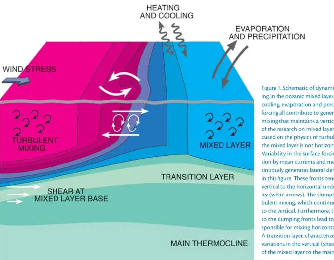
Figure 1. Schematic of dynamical processes act- ing in the oceanic mixed layer. Surface heating and cooling, evaporation and precipitation, and wind forcing all contribute to generating the turbulent mixing that maintains a vertically mixed layer. Most of the research on mixed layer dynamics has fo- cused on the physics of turbulent mixing. However, the mixed layer is not horizontally homogeneous.

Variability in the surface forcing and lateral advection by mean currents and mesoscale eddies continuously generates lateral density fronts, as shown in this ﬁ gure. Th ese fronts tend to slump from the vertical to the horizontal under the action of gravity (white arrows). Th e slumping opposes the turbulent mixing, which continuously restores fronts to the vertical. Furthermore, the accelerations due to the slumping fronts lead to local instabilities responsible for mixing horizontally across the fronts.

A transition layer, characterized by large velocity variations in the vertical (shears), connects the base of the mixed layer to the main thermocline.

The mixed layer is a complex dynamical environment that plays host to a large variety of physical phenomena. In broad terms, variability in the surface mixed layer results from a combination of processes arising from three fundamental sources: (1) atmospheric forcing, (2) motions in the ocean interior, (3) and their interactions (Figure 1). The fi rst two are reasonably well understood. The general characteristics of the ocean re- sponse to atmospheric forcing—surface fl uxes of momentum, heat, salt, and other tracers through the air-sea interface—

are described through one-dimensional

models. These models suppose that the properties of the surface layer are set by vertical mixing caused by mechanical stirring from the wind, surface gravity wave breaking, Langmuir circulations, and by convective mechanisms induced by buoyancy loss to the atmosphere (Csanady, 2001). Motions in the ocean interior—the structure and variability of mean currents and mesoscale eddies—are the subject of a vast literature (Gill, 1982). The energy in eddy motions is an order of magnitude larger than that in the mean currents, and dominates the temporal and spatial variability of the

ocean circulation. Furthermore, tran- sient motions have been shown to be important in setting the density stratifi - cation in the thermocline.

The contributions of atmospheric forcing and mesoscale motions to the upper ocean structure are clearly vis-

Raﬀ aele Ferrari ([email protected]) is Victor Starr Assistant Professor of Physical Oceanography, Massachusetts Institute of Technology, Cambridge, MA. Giulio Boc- caletti is Postdoctoral Research Associate, Massachusetts Institute of Technology, Cambridge, MA.

(4)

Latitude

Depth (m)

25 26 27 28 29 30 31 32 33 34 35

0

50

100

150

200

250

300 24.5

25 25.5

26 26.5

Potential Density (kg/m³)

Figure 2. Potential density section of the upper ocean from the Northeast Pacifi c along 140°W, measured in February 1997 by Rudnick and Ferrari (1999) as part of the Spice research campaign. Th e data resolution is 3 km in the horizontal and 8 m in the vertical. Th ere is a well- developed mixed layer in the upper 100-150 m. Th e mixed layer is a boundary layer at the ocean surface, maintained well mixed by the vertical fl uxes caused by the atmospheric forcing. Th e mixed layer base, defi ned by a 0.1 kg/m³ diff erence from the shallowest measure- ment, is indicated by the black line. Th e mixed layer base variations are due to vertical motions associated with mesoscale eddies in the ocean interior. Notice that the mixed layer is not uniform in the horizontal: lateral density fronts are the result of the interactions among surface forcing, mesoscale motions, and vertical mixing. Reprinted with permission, Rudnick and Ferrari (1999), copyright 1999 AAAS.

ible in high-resolution surveys. Figure 2 is a section of potential density from the Northeast Pacifi c (140°W, 25-35°N) obtained by Rudnick and Ferrari (1999) in February 1997 as part of the oceano- graphic campaign Spice. Temperature, salinity, and pressure were measured using a conductivity-temperature-depth (CTD) instrument aboard the towed, undulating vehicle SeaSoar. There is a well-developed mixed layer in the up-

per 100-150 m, which is vertically mixed by the turbulent fl uxes associated with atmospheric forcing. Horizontal fl uctuations in mixed layer depth are often mirrored by isopycnal doming below the mixed layer, as occurs in regions between 29° and 30° N. This doming is the result of vertical motions associated with deep mesoscale eddies that extend up into the mixed layer.

While the near-surface expression

of mesoscale eddies is clear in sections such as that shown in Figure 2, and even in satellite pictures of sea-surface temperature and sea-surface elevation, comparatively little is known about how vertical mixing and the thermocline mesoscale fl ows interact. This interplay has a twofold impact on upper ocean dynamics: (1) it modulates the air-sea fl uxes creating horizontal variability in tracer distributions, in near surface

(5)

stratifi cation, and in mixed layer depth, and (2) it modifi es the vertical transport by turbulent motions, therefore affecting exchanges with the oceanic interior (see schematic in Figure 1). These impacts are not negligible and contribute signifi - cantly to the budgets of both atmospheric and oceanic properties. Thus, atmospheric forcing and mesoscale motions considered in isolation of each other cannot capture the detailed structure of the mixed layer, nor accurately represent its role in the coupled system. This paper describes some of the recent advances in observing and understanding the physics of that interaction.

MESOSCALE AND SUBMESOSCALE DYNAMICS IN THE MIXED LAYER Turbulent motions generated by air-sea fl uxes maintain the surface boundary layer well mixed in the vertical. Horizon- tal eddy motions modulate the air-sea interface and introduce lateral variability in the fl uxes to and from the atmosphere (Figure 1). Heat fl uxes, for instance, de- pend critically on sea surface temperatures, which are substantially infl uenced by the advection of anomalously cold or warm water by eddies. The turbulent motions do not act directly on the ensuing temperature anomalies. Rather, the stirring by mesoscale eddies deforms the anomalies into thin fi laments. These fi laments become unstable, because they are associated with strong horizontal density gradients, and tend to slump. The restratifi cation associated with the slumping interacts in turn with vertical turbulent mixing. Evidence of the slumping instabilities and their interactions with

10¹ 10² 10³ 10⁴ 10⁵

10^-12 10^-10 10^-8

Scale [meters]

E(l) ≈ l⁰

E(l) ≈ I^-1

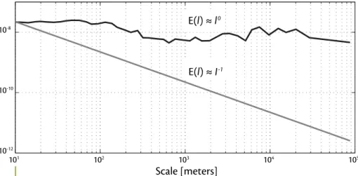
Figure 3. Intensity of temperature fl uctuations at diff erent horizontal scales l, as measured by towing a temperature sensor at a fi xed depth of 50 m in the mixed layer shown in Figure 2. Th e vertical axis represents the variance of temperature fl uctuations per unit length scale, E(l), in °C²/m.

Th e total variance of temperature is given by the integral of the area under E(l). Th e variance from data is plotted as a black line and is nearly constant for scales between 10 m and 100 km. If temperature was stirred only by mesoscale eddies in the surface mixed layer, one would expect E(l) to diminish with scale as shown by the gray line. Th e discrepancy between the two curves is due to the presence of atmospheric forcing and lateral submesoscale instabilities that interact with the eddy ﬁ eld and modify the temperature distributions.

mixing is diffi cult to produce, because the velocity fi elds associated with these processes cannot be measured directly in a system as noisy as the oceanic mixed layer. However indirect measurements such as satellite observations, tracer distributions, and data from both moorings and SeaSoar tracks, open a window on the variety of processes present.

The distribution of “tracers” (such as temperature, salinity, nutrient, and oxy- gen concentrations) offer a useful insight into the properties of horizontal motions in the mixed layer. In particular, the amplitude of tracer fl uctuations can be used to infer the structure of the velocity fi eld at different spatial scales. One introduces the tracer spectrum, that is,

the tracer variance per unit scale l at different horizontal scales l. Thus, the peak- to-peak tracer fl uctuations at each scale l are given by the spectrum multiplied by l. If mesoscale eddies generated in the main thermocline were responsible alone for the stirring in the mixed layer, we would expect the tracer spectrum to decrease with spatial scale as l^-1 and the corresponding tracer fl uctuations to be independent of spatial scale (Salmon, 1998). Instead, observations from in- struments towed at a fi xed depth in the mixed layer suggest that the spectrum does not decrease with depth on horizontal scales between 100 km and 10 m, as shown in Figure 3. The corresponding tracer fl uctuations grow as l with

(6)

Latitude

Depth (m)

35.4 35.6 35.8 36 36.2 36.4

0 50 100 150 200 250 300 350

Potential Density (kg/m³)

26.4 26.5 26.6 26.7 26.8 26.9 27 27.1 27.2

spatial scale. Therefore mesoscale eddies do not dominate the horizontal dynamics of the mixed layer at all scales, rather submesoscale motions and air-sea fl uxes are responsible for stirring and mixing tracers horizontally at scales shorter than 100 km.

A good place to start understanding the nature of submesoscale motions is with frontal structures. Fronts are generated where the mean currents or the mesoscale eddies bring together water masses with different temperatures and salinities. A textbook example is the permanent Azores Front in the North Atlantic shown in Figure 4 (Rudnick

and Luyten, 1996). These fronts exhibit hydrodynamic instabilities that manifest themselves in unstable waves and fi la- mentation at the submesoscale. These instabilities are dynamically different from ordinary baroclinic instability—responsible for producing mesoscale eddies—as they occur in an environment with weak density stratifi cation and vigorous vertical mixing. Submesoscale instabilities energize turbulent fl ows across the lateral density gradients and drive water mass conversion in the mixed layer. This happens through the generation of temperature, salinity, and other tracer gradients at progressively smaller scales, which

Figure 4. A density section across the Azores Front in the North Atlantic surveyed in March 1992 towing a SeaSoar vehicle equipped with a CTD. Fronts in density, such as the Azores Front, are usually accompanied by hydrodynamical instabilities that tend to slump the front and transport waters across the density gradient. Th e dynamics of these instabilities play an important role in redistributing tracer properties in the surface mixed layer. Figure from Rudnick and Lutyen (1996).

slump, generating regions of high velocity shear that are ultimately unstable to three-dimensional Kelvin-Helmholtz overturns.

These dynamics are not exclusive to large-scale frontal regions. Instabilities of the kind described above populate scales between 100 km and a few hundred meters in the mixed layers of the global oceans. Unlike the case of mesoscale eddies, which tend to coalesce and organize themselves into larger scale motions, submesoscale slumping transfers energy to smaller scales so that these motions are critically linked to their ultimate ar- rest by small-scale, three-dimensional

(7)

turbulent mixing. It is through these processes that the mixed layer mediates the interaction between turbulent mixing and mesoscale eddies.

Evidence that submesoscale motions are ubiquitous comes from a variety of sources. Where surface conditions allow for detection, satellite imagery shows that the ocean is populated with structures at these scales (between 100 km and 100 m) (Munk et al., 2000). Another important and convincing piece of evidence comes from the well-documented phenomenon of density compensation, especially during the winter. The density of seawater is determined by two properties: temperature and salinity. Typically, variations of temperature and salinity generate variations in density. It is, how-

ever, possible to have temperature and salinity fronts with no signature in density. This happens if a front is cold and fresh on one side and warm and salty on the other, so that temperature and salinity have opposing effects on density and are said to compensate. One of the most striking features of the winter mixed layer is that temperature and salinity compensate at almost all scales smaller than mesoscale structures. Figure 5 shows temperature and salinity profi les, measured by towing sensors at a fi xed depth of 50 m in the middle of the mixed layer along the whole section shown in Figure 2. Every change in temperature is mirrored by a corresponding change in salinity that compensates its effect on density. This pattern is visible on scales as

large as 10 km and as small as 10 m. The implication is that horizontal processes in the mixed layer work to eliminate horizontal density, but not to eliminate compensated gradients. Temperature and salinity fronts are generated through air-sea fl uxes and mesoscale stirring. At some locations these gradients compensate, whereas at other locations they cre- ate horizontal density gradients. Hori- zontal density gradients are unstable and tend to slump, tilting from the vertical to the horizontal. In the winter, turbulence is strong and thus subsequent vertical mixing results in a weakening of the horizontal density gradient. On the other hand, those fronts that are compensated do not slump and are, therefore, stable.

The net result of the interaction between

25 26 27 28 29 30 31 32 33 34 35

16 18 20 22

Latitude

θ (°C)

33 34 35 36

S (psu)

Figure 5. Potential temperature and salinity profi les measured when towing sensors from 25°N to 35°N at a fi xed depth of 50 m below the surface, right in the middle of the mixed layer shown in Figure 2. Th e vertical axes are scaled by the thermal and haline expansion coeffi cients so that equal excursions of temperature and salinity imply identical eff ects on density. Note that nearly every feature in temperature is mirrored by one in salinity at all scales. Temperature and salinity structure compensate to produce very small density gradients. Reprinted with permission, Rudnick and Ferrari (1999), copyright 1999 AAAS.

(8)

submesoscale instabilities and turbulent vertical mixing is that density fronts dif- fuse away, while compensated fronts per- sist much longer.

Although density compensation dominates in winter, during the sum- mer, when atmospheric forcing is weak, the restratifi cation due to slumping fronts can suppress vertical mixing and reduce the mixed layer depth. This leads to further evidence for the importance of submesoscale horizontal motions, as it is known that one-dimensional models tend to overestimate the mixed layer depth in weak mixing conditions, because they neglect the restratifi cation due to lateral instabilities.

Internally generated instabilities only account for part of the horizontal submesoscale motions in the mixed layer. Other notable sources of variability—

which we only mention here—include the nonlinear effects associated with the interaction of wind forcing and eddies.

The effect of wind forcing, whether it be inertial resonance or lower-frequency Ekman pumping, can be substantially modifi ed by the underlying velocity fi eld produced by the mesoscale eddy fi eld. The modulation of inertial oscilla- tions by the mesoscale eddy fi eld introduces variability in the high-frequency wind-driven shear and in the ensuing shear-driven vertical mixing. The super- position of wind-driven Ekman and mesoscale fi elds give rise to submesoscale circulations involving signifi cant vertical transports in and out of the mixed layer.

THE TR ANSITION L AYER The presence of horizontal motions at meso- and submesoscales also modifi es the vertical turbulent transfer of properties between the mixed layer and the oceanic interior. The mixed layer base is an important boundary, separating the weakly stratifi ed surface waters from the highly stratifi ed interior (Figure 1).

While turbulent mixing does decay with depth, it does not disappear at the mixed layer base, contrary to the traditional no- tion of the mixed-layer base as a boundary between quiescent and turbulent regions. The transition layer is the region where mixing rates transit from high values in the mixed layer to extremely low values in the interior. This transition region is extremely important for the ventilation of the ocean because all sub- ducted tracers must pass through it, and are modifi ed in it, before joining the geo- strophic interior fl ow. For example, the temperature-salinity structure of the upper ocean differs remarkably from that found in the thermocline waters below.

Processes occurring at the mixed layer base are likely to play a signifi cant role in these changes.

Observations show that wind-driven momentum and shear (rate of change of velocity with depth) penetrate below the mixed layer. The penetration depth is typically a few tens of meters, but can occasionally extend to more than a hundred meters. It is an open question as to what determines the thickness of this transition layer: wind-driven shears

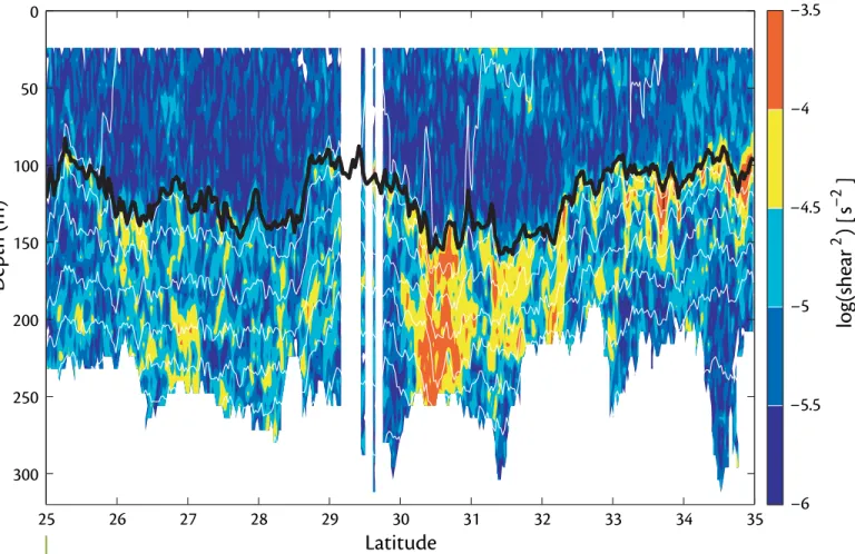
and instabilities generated in the mixed layer can have a signifi cant projection below and enhance/suppress vertical transports, therefore contributing to the dynamics below. What is clear though is that the transition layer is far from homogeneous in the horizontal. Figure 6 shows the magnitude of the shear in the same upper ocean section used in Figure 2. Shear is very weak in the mixed layer, where turbulent mixing tends to homogenize momentum in the vertical, while it is enhanced below the mixed layer base. There are localized patches where the enhanced shear penetrates down to 300 m, while in other regions the shear penetrates only a short distance below the mixed layer. The penetration depth is not simply proportional to the strength of the local wind fi eld at the surface: horizontal mesoscale and submesoscale motions modify the wind-driven motions as they radiate from the surface.

While shear and mixing processes are often described as one dimensional involving the vertical energy balance of the water column, horizontal eddy motions on a wide range of scales modulate such processes signifi cantly. A passing disturbance, for instance, can temporar- ily modify the stratifi cation of the water column or the vertical transport, therefore changing the background state upon which the vertical processes act. This might change signifi cantly the rates of water exchanges between the mixed layer and the interior, and affect the global budgets of the exchanged properties.

(9)

Figure 6. Velocity shear squared for the ocean section shown in Figure 2. Th e shear is the velocity change per unit vertical distance. Th e shear shown in this ﬁ gure is computed across vertical intervals of 8 m. Th e black line denotes the mixed layer base, deﬁ ned as a 0.1 kg/

m³ change from the surface value. Th e shear is very weak in the mixed layer because vertical mixing tends to homogenize momentum and remove any velocity change. Shear is instead high below the mixed layer, in the transition layer. (Notice however that there is some shear in the mixed layer. A comparison of shear and density stratifi cation in the mixed layer shows that density is better homogenized than momentum. Th is diff erence is due to Earth’s rotation, which generates shears in the presence of horizontal density gradients.) Th e maximum values of shear are right at the mixed layer base, and only occasionally penetrate deeper than a few tens of meters below this base. Th e high shears in the transition layer generate density overturns and produce mixing. Th e mixing rates are, however, smaller than in the mixed layer, and do not eliminate completely the density stratifi cation.

Latitude

Depth (m)

25 26 27 28 29 30 31 32 33 34 35

0

50

100

150

200

250

300

−6

−5.5

−5

−4.5

−4

−3.5

log(shear2 ) [s−2 ]

NUMERICAL MODEL S OF THE UPPER O CE AN

This cursory survey of upper ocean dynamics has shown that mesoscale, submesoscale, and turbulent processes interact and control the lateral and vertical transport of tracers and momentum

at the ocean surface. Thus, the large-scale circulation in the upper ocean depends crucially on motions with scales between 100 km and a few meters. Given the limi- tations of today’s computers, numerical models used for climate studies cannot afford to resolve the full range of oceanic

motions, and thus must resort to parameterizing the effect of small-scale motions on the larger scales. The challenge is then to fi nd mathematical operators that accomplish the necessary physical effects associated with unresolved small- scale motions, so as to obtain closed

(10)

equations for the large-scale circulation.

In present climate models, the ocean horizontal grid resolution is O(100) km or larger. At this resolution, mesoscale and submesoscale eddy dynamics, and turbulent boundary mixing must all be parameterized. A number of parameter- ization schemes have been proposed to represent the effects of mesoscale eddies in the ocean interior. One-dimensional models have been derived to parameter- ize air-sea fl uxes and boundary-layer turbulence. Unfortunately our poor understanding of the interactions between these two classes of motion has hampered attempts to derive closure schemes that account for both. The com- mon practice is to use parameterizations for mesoscale motions only in the ocean interior, where turbulence is weak and does not affect larger-scale motions.

Mesoscale and submesoscale eddies are instead ignored in the boundary layers, where parameterizations account only for turbulent mixing processes. As discussed above, this is at odds with the observational and theoretical evidence that eddy fl uxes have a strong impact on upper-ocean dynamics.

Until these issues have been adequate- ly addressed, coupled climate models will be severely limited in simulating air-sea interactions. Some progress is expected in the near future thanks to a project recently sponsored by the National Sci- ence Foundation and the National Oce- anic and Atmospheric Administration.

The project comprises a group of fi fteen leading oceanographers organized in a Climate Process Team that works in close

collaboration with modeling centers in Princeton and Boulder. The group is using a combination of theory and observations of the kind described above to derive parameterizations of eddy- mixed layer interactions suited for ocean models used in climate studies. More- powerful computers will appear in the future and may permit decreasing the horizontal resolution to O(10) km in the next decade. At this resolution mesoscale eddies will be partly resolved. However, the interactions between mesoscale eddies and turbulent fl uxes in the mixed layer happen at much smaller scales and need to be parameterized even at O(10) km resolution. Thus, the problem of understanding and parameterizing eddy- mixed layer interactions will remain a critical issue for climate studies in the near future.

CONCLUSION

The oceanic mixed layer plays a fundamental role in climate because it controls the exchange of heat, freshwater, carbon dioxide, and many other properties between the ocean and the atmosphere. It is therefore no surprise that this layer has been the focus of oceanography since the pioneering work of V. Walfrid Ekman at the beginning of last century. (Ekman was a Swedish physical oceanographer best known for his studies of the dynamics of ocean currents and who is credited with recognizing the role of the Coriolis effect on ocean currents.) However, only in the last decade have observations of the three-dimensional structure of the mixed layer become available. Instru-

ments mounted on SeaSoar towing ve- hicles, ocean gliders, fl oats, drifters, and moorings are shedding light on a wide range of phenomena never observed before, revealing an unexpected complexity. While these data pose a challenge for modelers and theoreticians alike, they are reinvigorating the fi eld as new puz- zling pieces of evidence appear with in- creasing frequency in scientifi c journals.

It is indeed an exciting time for the fi eld, and we hope that many of the issues raised in this article will soon fi nd an explanation through the combined effort of observationalists, numerical modelers, and theoreticians.

ACKNOWLED GE MENT

The authors acknowledge the support of the National Science Foundation under awards OCE02-4152 and OCE03-36755.

REFERENCE S

Csanady, G.T. 2001. Air-Sea Interaction. Cambridge University Press, 284 pp.

Gill, A. 1982. Atmosphere-Ocean Dynamics. Aca- demic Press, San Diego, 662 pp.

Munk, W., L. Armi, K. Fischer, and F. Zachariasen.

2000. Spirals in the sea. Proceedings of the Royal Society of London 456(Series A):1217-1280.

Rudnick, D.L., and R. Ferrari. 1999. Compensation of horizontal temperature and salinity gradients in the ocean mixed layer. Science 283:526-529.

Rudnick, D.L., and J.R. Luyten. 1996. Intensive surveys of the Azores Front: 1, Tracers and dynamics. Journal of Geophysical Research 101:923-939.

Salmon, R. 1998. Geophysical Fluid Dynamics. Ox- ford University Press, New York, 378 pp.