AhigherorderRoot-MUSICanditsrealpolynomialform 高次 Root-Music とその実多項式形

社団法人 電子情報通信学会

THE INSTITUTE OF ELECTRONICS,

INFORMATION AND COMMUNICATION ENGINEERS

信学技報

TECHNICAL REPORT OF IEICE.

高次 Root-Music とその実多項式形

曹 祥 ^† 上手 洋子 ^† 西尾 芳文 ^† 辛 景民 ^††

† ^{徳島大学工学部 〒} 770–8506 徳島県徳島市南常三島町 2-1

†† Xi’an Jiaotong University No.28 Xianning West Road, Xi’an 710049, China E-mail: †{ caoxiang, uwate, nishio } @ee.tokushima-u.ac.jp, †† [email protected]

あらまし 本研究では， Root-MUSIC 到来方向推定法の実多項式を提案する．共形変換を用いて Root-MUSIC を実係 数多項式への変換を行う． そして，上半単位円上の変数を用いた高次 Root-MUSIC の提案を行う．提案手法は J. Selva 2005 の手法より優れた性能を示した．

キーワード パラメータ概算， ULA ，アレイ信号処理

A higher order Root-MUSIC and its real polynomial form

Xiang CAO ^† , Yoko UWATE ^† , Yoshifumi NISHIO ^† , and Jingmin XIN ^††

† Department of Electrical and Electronic Engineering, Tokushima University 2-1 Minami-Josanjima, Tokushimashi, Tokushima, 770-8506, Japan

†† Department of Institute of Artificial Intelligence and Robotics, Xi’an Jiaotong University No.28 Xianning West Road, Xi’an 710049, China E-mail: †{ caoxiang, uwate, nishio } @ee.tokushima-u.ac.jp, †† [email protected]

Abstract This paper presents a real polynomial form of the popular Root-MUSIC direction-of-arrival (DOA) algorithm. To transform Root-MUSIC into real coefficients polynomial with the help of conformal transformation, we propose a higher order Root-MUSIC whose variable is only defined on the unit upper semicircle. Furthermore, this paper also improves the results obtained by J.Selva in 2005.

Key words Parameter estimation, uniform linear array (ULA), array signal processing

1. Introduction

The multiple signal characterization (MUSIC) algorithm for direction finding [1] has been advanced for many years.

To a certain degree, the more search points one use, the more accurate results one will obtain. The main computa- tional burden locate the process of spectral search. Thus, many efficient methods are proposed to reduce the search complexity of spectral MUSIC.

To avoid the tremendous computation load of spectral search, Root-MUSIC [2], [3] was proposed. The search-free method has an improved resolution threshold relative to con- ventional MUSIC. Taking advantage of conformal transfor- mation, the author of [4] translated the Root-MUSIC into an univariate polynomial with real coefficients. Here, we have to point out that the interested spatial frequency in Root- MUSIC lies in the interval [−π, π] instead of [0, π]. Since only half of field-of-view is considered, the real coefficients polyno-

mial in [4] has the same degree with standard Root-MUSIC.

In this paper, we improve the result and give the real poly- nomial form of Root-MUSIC in [−π, π]. The same mapping idea also appears in [5] to estimate single target. In [5], the interested range is mapped into real line by a tangent func- tion, while the transformation function is not monotonic over target range. That is to say, the target may not be uniquely determined from the inverse transformation.

In this paper, we propose a higher order Root-MUSIC whose variable is only defined on the unit upper semicir- cle. The similar Root-MUSIC then is transformed into real polynomial form. Our method treats the whole range of in- terest in uniform linear array (ULA). The process of solving this polynomial just involves real arithmetic [6]. This method also can be used in unitary Root-MUSIC [7] and unitary MU- SIC [8].

— 1 —

2. Data Model

Assume p far-field narrowband signals {s

} impinging on a ULA with M (M > p) sensors. The output vector y(t) of the array at time t can be written as

y(t) = A(θ)s(t) + n(t), (1) where s(t) is the vector of incident signals and n(t) is the vector of additive noises. The so-called array steering matrix and steering vector have the following form:

A(θ) = [a(θ

), a(θ

), · · · , a(θ

)22] (2)

a(θ

) = h

1, e

, · · · , e

π

λ(M−1)dsin(θi)

i

, (3)

here, (·)

denotes transpose operator, d and λ stand for the distance between two consecutive sensors and the iden- tical wavelength for all signals, respectively. The restriction of Directions-of-arrival (DOAs) θ

, · · · , θ

lie in the inter- val

−

,

for the purpose of eliminating the ambiguity of ULA [9].

Next, we define spatial frequency ω

=

d sin(θ

). Then, (3) becomes

a(ω

) = h

1, e

, · · · , e

i

. (4)

For guaranteeing the uniqueness of a(ω

), i = 1, 2, · · · , p, the spatial frequency ω

are in [−π, π] instead of [0, π] in [4]. In other words, the author in [4] only consider the half of the DOA range of interest. Since the one-to-one correspondence between ω

and θ

, we only focus on the problem of estimat- ing parameters ω

, i = 1, 2, · · · , p in this paper.

3. Real polynomial form of Root-MUSIC

Under the assumptions of the uncorrelated signals and the white Gaussian noise, the array covariance matrix can be decomposed into

R = E{y(t)y

(t)} = U

Λ

U

+ U

Λ

U

. (5) It is clear that the columns of A(θ) have the maximum pro- jection on the signal subspace U

and are orthogonal to the noise subspace U

. With this observation, two natural esti- mation criterions are to find the local maxima or minima [1], viz.

ˆ

ω = arg max

ω f

(ω) = arg max

ω a

(ω)U

U

a(ω) (6) or

ˆ

ω = arg min

ω f

(ω) = arg min

ω a

(ω)U

U

a(ω). (7) The total number of complex flops in (6) is Jp(2M +1) and the one in (7) is J(M −p)(2M +1) [10], where J (J ≫ M > p)

is the number of spectral search points. Nevertheless, the subspace decomposition in (5) costs O(M

p) complex flops [11], [12]. We can conclude that the main computational load of spectral MUSIC is the search steps. Consequently, it is necessary to reduce the complexity of spectral search process.

Next, we will deduce the real polynomial form of Root- MUSIC with the help of conformal transformation. By defin- ing a translation

z = e

, (8)

the real point ω belonging to the domain [−π, π] can be mapped to the unique complex point z belonging to the unit upper semicircle. Furthermore, let us introduce a conformal transformation

u = −j z − j

z + j . (9)

The above function is a one-to-one mapping that takes the unit upper semicircle to the interval [−1, 1] of real line [4], [5], [13]. Substituting (8) into (9), we get the relationship between ω ∈ [−π, π] and u ∈ [−1, 1] as follows:

u = tan ω 4

. (10)

This is a monotonic function in [−π, π] and its range is [−1, 1]. Thus, once the variable u is estimated, the unique spatial frequency ω can be obtained by ω = 4 arctan u. For this purpose, the array vector response a(ω) must be con- nected to u.

Using z = −j

and e

= −z

( the two equations can be easily obtained from (8) and (9) ), we get

[a(ω)]

= e

= (−1)

z

= u − j

u + j

, m = 1, 2, · · · , M. (11) Multiplying by (u + j)

(here, we note u = | −j ), the above equation then becomes

(u + j)

[a(ω)]

=(u − j)

(u + j)

= c

u

+ · · · + c

= c

v(u), m = 1, 2, · · · , M (12) where the (2M − 1) × 1 coefficient vector c

= [c

, c

,

· · · , c

]

can be calculated by convolution operation [5], [14], v(u) = [1, u, · · · , u

]

is unknown real vector.

Let us define an M ×(2M −1) matrix C = [c

, c

, · · · , c

]

, the array steering vector a(ω) can be expressed

a(ω) = (u + j)

Cv(u). (13) In ULA, the Root-MUSIC always has more resolution com- pared with spectral MUSIC [3]. Thus, it is interesting to look for a real polynomial form of Root-MUSIC. Using z = e

,

— 2 —

ω ∈ [0, π] and (9), a real polynomial with degree 2(M − 1) has been obtained in [4]. However, If we consider the whole domain ω ∈ [−π, π], the conformal transformation equation (9) will not exist in z = e

, but exists in (8).

Thus, we can define the mth element of vector a(z) as follows:

[a(z)]

= (−1)

z

, m = 1, 2, · · · , M. (14) The function f

(ω) in (7) then becomes

f

(z) = a

(z)U

U

a(z) = 0. (15) This is a polynomial of degree 4(M − 1) with complex coeffi- cients and the variable z is defined on the unit upper semicir- cle instead of the entire unit circle in the conventional Root- MUSIC with 2(M − 1)-degree complex coefficients. Using the equation a(z ) = (u + j)

Cv(u) , we get

v

(u)C

U

U

Cv(u) = 0. (16) The roots of polynomial in (15) appear in reciprocal pairs z,

[9] and could not be on the unit circle because of the effects of noise. The pair roots are related to u by conformal transformation (9),

u

= −j z − j

z + j , u

= −j 1 − jz

1 + jz

. (17)

Obviously, we have u

= u

. It is reasonable to conclude that the roots in (16) also appear in conjugate pairs like (u, u

).

As a consequence, the equation (16) is a real coefficients polynomial, namely

v

(u)Re n

C

U

U

C o

v(u) = 0. (18) Next, we will analyze how to estimate the spatial frequency ω

, i = 1, 2, · · · , p from the conjugate roots (u

, u

) , i = 1, 2, · · · , 2(M − 1) of the above polynomial. Assuming z = a + jb, b > = 0, the equation (9) becomes

u = −j a + jb − j

a + jb + j = −2a − j a

+ b

− 1

a

+ (b + 1)

. (19) When the roots z in (15) are close to the unit circle, the imaginary part of u must tend to zero. Therefore, p real parts of u

can be picked up through comparing the absolu- tion value of imaginary part of u

, i = 1, 2, · · · , 2(M −1). The spatial frequency will be given by ω

= 4 arctan [Re (u

)] , i = 1, 2, · · · , p.

Note that, although the polynomial in (18) have 4(M −1)- degree, its coefficients are real and roots appear in conjugate pairs. Thus, we only need to solve 2(M − 1) roots. For real polynomial, the process of solution can avoid all complex arithmetic using Bairstow’s method [6]. In practice, finding roots of a function usually involve iteration. The operation in (18) is O(16M

) real flops per iteration, while the Root- MUSIC requires O(24M

) real flops per iteration (1 com- plex flop = 6 real flops) even though polynomial have degree 2(M − 1).

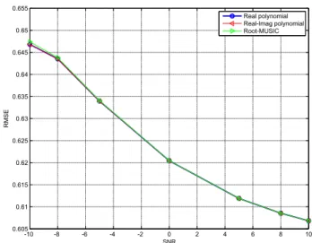
-10 -8 -6 -4 -2 0 2 4 6 8 10

0.605 0.61 0.615 0.62 0.625 0.63 0.635 0.64 0.645 0.65 0.655

SNR

RMSE

Real polynomial Real-Imag polynomial Root-MUSIC

図

1 RMSE of spatial frequency ω =-0.3. The number of snap- shots N = 100

4. EXPERIMENTS

In this section, an examples was conducted by computer simulation. In all scenarios, two equal-power uncorrelated signals are considered and a ULA have 9 sensors. Mean- while, we set spatial frequency ω

= −0.3, ω

= 1.2. Here, ω

can not be solved in [4].

Example: Performance of real polynomial based on Root- MUSIC

In this case, we mainly test the validity of real coefficients polynomial (18). For this purpose, let us introduce the imag- inary part of matrix H = C

U

U

C. After simple deriva- tion, we obtain

v

(u) {Re {H} + Im{H}} v(u) = 0. (20) This approach using (20) named real-imag polynomial and was indicated by red line in Figure. 1. It is worth pointing out that (18) and (20) give the same results. That is to say, the coefficients of polynomial (16) are real. Meanwhile, the behavior of our method have been improved a little at lower signal-to-noise ratio (SNR) than Root-MUSIC [2].

5. CONCLUSIONS

For improving the results in [4], we propose a higher order Root-MUSIC whose variable is only defined on the unit up- per semicircle. Then, the complex equation is transformed into real polynomial form with the help of conformal trans- formation. The process of solution can avoid all complex arithmetic.

References

[1] R. O. Schmidt, “Multiple emitter location and signal pa- rameter estimation,” IEEE Trans. Antennas Propag., vol.

53, pp. 276–280, Mar. 1986.

[2] A. J. Barabell, “Improving the resolution performance of eigenstructure-based direction-finding algorithms,” in Proc.

— 3 —

ICASSP, Boston, MA, May 1983, pp. 336–339.

[3] B. D. Rao and K. V. S. Hari, “Performance analysis of root- music,” IEEE Trans. Acoust.,Speech, Signal Process., vol.

37, pp. 1939–1949, Dec. 1989.

[4] J. Selva, “Computation of spectral and root music through real polynomial rooting,” IEEE Trans. Signal Process., vol.

53, pp. 1923–1927, May 2005.

[5] J. X. Wu, T. Wang, and Z. Bao, “Fast realization of max- imum likelihood angle estimation with small adaptive uni- form linear array,” IEEE Trans. Antennas Propag., vol. 58, pp. 3951–3960, Dec. 2010.

[6] W. H. Press, S. A. Teukolsky, W. T. Vetterling, and B. P.

Flannery, Numerical recipes in C, Cambridge Univ. Press, Cambridge, U.K., 1997.

[7] M. Pesavento, A. B. Gershman, and M. Haardt, “Unitary root-music with a real-valued eigendecomposition: a theo- retical and experimental performance study,” IEEE Trans.

Signal Process., vol. 48, pp. 1306–1314, May 2000.

[8] K. C. Huarng and C. C. Yeh, “A unitary transformation method for angle-of-arrival estimation,” IEEE Trans. signal process., vol. 39, pp. 975–977, Apr. 1991.

[9] P. Stoica and R. L. Moses, Spectral analysis of signals, Prentice-Hall, 2005.

[10] D. S. Watkins, Fundamentals of matrix computations, Wi- ley, 2004.

[11] Y. Zhang and B. P. Ng, “Music-like doa estimation with- out estimating the number of sources,” IEEE Trans. Signal Process., vol. 58, pp. 1668–1676, Mar. 2010.

[12] F. G. Yan, M. Jin, and X. Qao, “Low-complexity doa es- timation based on compressed music and its performance analysis,” IEEE Trans. Signal Process., vol. 61, pp. 1915–

1930, Apr. 2013.

[13] L. Blanco, J. Serra, and M. N´ ajar, “Conformal transfor- mation for efficient root-toa estimation,” in Proc. ISCCSP, Malta, Mar. 2008, pp. 1314–1319.

[14] M. Costa and V. Koivunen, “Incorporating array nonideal- ities into adaptive capon beamformer for source tracking,”

in Proc. SAM, Hoboken,NJ, Jun. 2012, pp. 445–448.

— 4 —