Study of Fusion Barrier Distributions from Quasielastic Scattering Cross Sections

(1)

九州大学学術情報リポジトリ

Kyushu University Institutional Repository

超重核合成に向けた準弾性散乱による融合障壁分布の研究

田中, 泰貴

http://hdl.handle.net/2324/2236025

出版情報：Kyushu University, 2018, 博士（理学）, 課程博士バージョン：

権利関係：

(2)

Study of Fusion Barrier Distributions from Quasielastic Scattering Cross Sections

towards Superheavy Nuclei Synthesis

Taiki Tanaka

Department of Physics, Kyushu University

February 11, 2019

(3)

Abstract

The study of fusion barrier distributions is of fundamental importance in understanding heavy-ion induced fusion reaction toward synthesis of superheavy nuclei. Cross sections of the reactions for producing new elements are predicted to be much smaller than those for the existing elements. They are also known to be particularly sensitive to the incident energy. One of the most direct information for determining the optimum incident energy is the fusion barrier distribution.

This work aims at precisely obtaining the fusion barrier distribution of heavy-ion induced reactions by measuring the quasielastic scattering and at probing the re- lation between the barrier distribution and the optimum incident energy at which the evaporation residue cross section is maximized. Reactions studied in this work involve not only the cold fusion reactions traditionally used for the synthesis of new elements withZ =107−113, but also the hot fusion reactions recently being used for the synthesis of new elements heavier than Z = 114. Eﬀects of channel coupling and deformation of the target nucleus on the barrier distributions are discussed.

Many quasielastic scattering measurements were performed at RIKEN Nishina Center for Accelerator-Based Science using the gas-filled recoil ion separator GARIS to improve our understanding of fusion reactions. What is new in this method is measuring the recoiled nuclei at completely forward side using GARIS.

This method enable to derive the barrier distribution for angular momentuml=0 concern with superheavy nuclei synthesis. The excitation functions of quasielastic scattering cross-section of ⁴⁸Ca+²⁰⁸Pb, ⁵⁰Ti+²⁰⁸Pb, ⁴⁸Ca+²³⁸U, ²²Ne+²⁴⁸Cm,

26Mg+²⁴⁸Cm,³⁰Si+²⁴⁸Cm,³⁴S+²⁴⁸Cm,⁴⁰Ar+²⁴⁸Cm,⁴⁸Ca+²⁴⁸Cm and⁵⁰Ti+²⁴⁸Cm were determined.

The quasielastic barrier distributions were extracted for the 10 reaction systems previously noted, and were compared to coupled-channels calculations, and were compared to evaporation residue cross-sections. The calculation results indicate that the deformation of actinoide target nucleus, the vibrational and rotational excitations of the colliding nuclei, as well as neutron transfers before contact, aﬀect the structure of the barrier distribution. The peak of the 2n evaporation cross-section of the cold fusion reactions ⁴⁸Ca+²⁰⁸Pb and ⁵⁰Ti+²⁰⁸Pb – relevant

(4)

to the synthesis of No (atomic number Z = 102), Rf (Z = 104) – emerged at the same energy as a local maximum of the barrier distributions. The evaporation cross-section of the hot fusion reactions ²²Ne+²⁴⁸Cm, ²⁶Mg+²⁴⁸Cm, ⁴⁸Ca+²³⁸U and ⁴⁸Ca+²⁴⁸Cm – relevant to the synthesis of Sg (Z = 106), Hs (Z = 108), Cn (Z = 112) and Lv (Z = 116), which are the frontier of the known superheavy nuclei – peak at an energy between experimental average Coulomb barrier height and the Coulomb barrier for a side collision. It is clear that the hot fusion reactions take advantage of a compact collision geometry with the projectile impacting the side of the deformed target nucleus.

The Coulomb barrier height of side collisions for synthesizing unknown superheavy nuclei were calculated using the experimental results from the barrier distribution study. New method for determining the incident energy for unknown superheavy nuclei using experimental results was proposed. This determination is independent of theoretical predictions that may include a large model dependence.

(5)

Chapter 1 Introduction

1.1 History of the new elements

From the ancient times, people have tried to understand the properties of the materials in nature. Ancient philosophers tried to think about the origin of the materials through rhetoric and logic alone. The elements began to be understood by experimental results in the 16^th - 17^th centuries[1]. The periodicity of the elements was noticed in the 18^th century[2]. The elements were arranged as a periodic table by Dmitri Ivanovich Mendeleev (1834 - 1907) in 1869, published in 1870.

The first particle accelerators, such as electrostatic accelerator (Van de Graaﬀ, 1931) linear accelerator (Lawrence and Sloan, 1931) cyclotron (Lawrence, 1932), were invented and developed in 1930’s[3]. Technetium (Tc, atomic numberZ = 43) was the first artificial element produced using a particle accelerator in 1937[3].

Scientists have been able to produce many artificial elements beyond those existing in nature. All of the elements which are heavier than uranium were dis- covered by artificial methods. Table 1.1 shows the reactions, investigators, and years of discovery for elements heavier than uranium. At this time, elements up to Z = 118 are recognized by international union of pure and applied chemistry (IUPAC). Scientists try to synthesize new elementsZ = 119 or 120 presently.

There are two methods for new element synthesis heavier thanZ = 102, so called “cold fusion reaction” and “hot fusion reaction”. The cold fusion reaction was used for new element synthesis between Z = 107 and 113, using spherical magic nuclei ²⁰⁸Pb or ²⁰⁹Bi as a target. The excitation energy of the compound nucleus is reduced by the reduced mass of the magic nuclei. The excitation energy is around 10 − 20 MeV, and the compound nucleus emits just 1 or 2 neutrons to make an evaporation residue without fission. The survival probability P_surv is much large compared to that of hot fusion reaction as a result of expeling a few

(9)

Table 1.1: Table of the informations of syntheses new elements. The informations based on Ref. [3]

Z Symbol Reaction Investigators Year

93 Np ²³⁸U(n,γ)²³⁹U→²³⁹Np MacMillanet al. 1939 - 1940 94 Pu ²³⁸U(d,2n)²³⁸Np→²³⁸Pu Seaborget al. 1940

95 Am ²³⁹Pu(2n,γ)²⁴¹Pu→²⁴¹Am Seaborget al. 1944

96 Cm ²³⁹Pu(α,n)²⁴²Cm Seaborget al. 1944

97 Bk ²⁴¹Am(α,2n)²⁴³Bk Seaborget al. 1949

98 Cf ²⁴²Cm(α,n)²⁴⁵Cf Seaborget al. 1950

99 Es ²³⁸U+15n→²⁵³Es Seaborget al. 1953

100 Fm ²³⁸U+17n→²⁵⁵Fm Seaborget al. 1953 101 Md ²⁵³Es(α,n)²⁵⁶Md Seaborget al. 1955 102 No ²⁴⁶Cm(¹²C,4n)²⁵⁴No Seaborget al. 1958 103 Lr ²⁵²Cf(¹¹B,6n)²⁵⁷Lr Ghiorsoet al. 1961 104 Rf ²⁴⁹Cf(¹²C,4n)²⁵⁷Rf Ghiorsoet al. 1969 105 Db ²⁴⁹Cf(¹⁵N,4n)²⁶⁰Db Ghiorsoet al. 1970

243Am(²²Ne,4n)²⁶¹Db Morlandet al. 1971 106 Sg ²⁴⁹Cf(¹⁸O,4n)²⁶³Sg Ghiorsoet al. 1974 107 Bh ²⁰⁹Bi(⁵⁴Cr,n)²⁶²Bh Armbrusteret al. 1981 108 Hs ²⁰⁸Pb(⁵⁸Fe,n)²⁶⁵Hs Armbrusteret al. 1984 109 Mt ²⁰⁹Bi(⁵⁸Fe,n)²⁶⁶Mt Armbrusteret al. 1982 110 Ds ²⁰⁸Pb(⁶²Ni,n)²⁶⁹Ds Armbrusteret al. 1995 111 Rg ²⁰⁹Bi(⁶⁴Ni,n)²⁷²Rg Hofmannet al. 1995 112 Cn ²⁰⁸Pb(⁷⁰Zn,n)²⁷⁷Cn Hofmannet al. 1996 113 Nh ²⁴³Am(⁴⁸Ca,3n)²⁸⁸Mc→²⁸⁴Nh Oganessianet al. 2004

243Am(⁴⁸Ca,4n)²⁸⁷Mc→²⁸³Nh Oganessianet al. 2004

209Bi(⁷⁰Zn,n)²⁷⁸Nh Moritaet al. 2004 114 Fl ²⁴²Pu(⁴⁸Ca,3n)²⁸⁷Fl Oganessianet al. 2004 115 Mc ²⁴³Am(⁴⁸Ca,3n)²⁸⁸Mc Oganessianet al. 2004

243Am(⁴⁸Ca,4n)²⁸⁷Mc Oganessianet al. 2004 116 Lv ²⁴⁵Cm(⁴⁸Ca,2n)²⁹¹Lv Oganessianet al. 2004 117 Ts ²⁴⁹Bk(⁴⁸Ca,3n)²⁹⁴Ts Oganessianet al. 2010

249Bk(⁴⁸Ca,4n)²⁹³Ts Oganessianet al. 2010 118 Og ²⁴⁹Cf(⁴⁸Ca,3n)²⁹⁴Og Oganessianet al. 2006

(10)

The hot fusion reactions were used for synthesizing new element 102 ≤ Z ≤ 106 and 114 ≤ Z ≤ 118. The reaction employed deformed actinide nuclei as a target. Since the excitation energy of a compound nucleus of hot fusion reaction is higher than that of cold fusion reaction, the reaction is called “hot fusion reaction”.

The compound nucleus releases 3 - 6 neutrons, then, the survival probabilityPsurv

is considerably smaller than that of cold fusion reaction. Both the cold and hot fusion reactions have some advantages and disadvantages.

1.2 Superheavy elements

1.2.1 Liquid drop model

Weizsacker[4] and Bethe[5] proposed the formula of Weizsaecker-Bethe. It is based on “liquid drop model”, and the model explained the characteristics of the nuclear binding energy well. In 1938, Otto Hahn irradiated uranium with neutrons. Then, he observed radium in the experimental result. He was not able to understand the reason. He sent a letter to Lise Meitner to find the reason. Lise Meitner explained the reason to him. Otto Hahn understood the mechanism of the fission from her explanation and got the Nobel prize in 1944. The fission barrier disappears toward superheavy element region in the liquid drop model. It means, superheavy elements do not have the stability against fission and should immediately undergo nuclear fission. In such a case, superheavy elements can not exist.

1.2.2 Shell model and macroscopic-microscopic model

Mayer[6] and Jensen[7] established the shell model in 1949. Strutinsky introduced the macroscopic-microscopic model in 1966. In that model, he adopted the liquid drop model as macroscopic part, and the shell model as microscopic part[8]. Figure 1.1 shows the calculated results of the macroscopic-microscopic model (solid lines) and liquid drop model (dashed line). In case of the liquid drop model, the fission barrier disappear at Z > 104. The fission barrier persists in the superheavy element region due to the shell eﬀect. In addition to above informations, the model explained the existence of the nuclear isomerism well. The possible existence of superheavy element was considered after introduction of this model. We were able to search for the superheavy elements more thanZ = 104.

(11)

Figure 1.1: Nuclear deformation energy (solid lines) and the liquid drop model deformation energy (dashed lines) for heavy nuclei. In case of the liquid drop model, the fission barrier disappear at Z > 104. Thanks to the shell eﬀect, the fission barrier appear not only Z ≤ 104 region but also superheavy elements region. This figure is taken from Ref. [8].

(12)

1.2.3 Quantum many body system

In the lectures of quantum mechanics, we learned about quantum tunneling. It is one of the most famous and original phenomena in quantum mechanics. However, I think, it is rare for this phenomenon to be seen in our real life. Since the superheavy nuclei have a lot of nucleons and make Coulomb barrier potentials which is made some of the nuclear potential and Coulomb potential, we are able to demon- strate the phenomenon using the superheavy nuclei. One focus of this thesis is the penetration of the Coulomb barrier, and the eﬀect of quantum tunneling is clearly seen.

In case of alpha decay study, the decay is caused by the penetration of the Coulomb barrier. Since the penetrability depends on the shape of the Coulomb barrier[9], such decay studies enable us to understand the nuclear structure in fine detail. The region of alpha decay is very limited, covering only the heavy and superheavy nuclei region. We are able to research nuclear structure in fine detail in superheavy nuclei region by synthesizing superheavy nuclei.

1.2.4 Frontier of the nuclei

Where is the next double magic nuclei beyond²⁰⁸Pb? Theoretical physicists have made multiple predictions for the next magic numbers[10, 11]. However, the predicted proton magic numbers diﬀer due to dependence on various models. Ac- cording to Fig. 1.2, the fission barrier heights in of the region of nuclei heavier than known nuclei is not high enough to allow existence of such nuclei. There- fore, we may have a little hope to make heavier nuclei than known superheavy nuclei. The Russian group, however, has clarified the evidence for an island of stability from the results of systematic studies in superheavy nuclei region[12].

From these systematic measurements of the superheavy nuclei, we might be able to reach the island of stability.

1.2.5 Importance for optimum incident energy

Figure 1.3 shows the evaporation residue cross sections for the reaction of⁴⁸Ca+²⁰⁸Pb as functions of center of mass energies. In this case, if the incident energy were changed by 1.6% (5%) from the optimum position, the cross-section would decreased to about one third (one order of magnitude lower). We would like to know the dependence of energy on cross-section, and it is valuable to perform synthesis studies at the optimal energy. However, in cases such as the synthesis of nihonium by cold-fusion, where 1 atom was seen for 200 days of beam on target, we cannot experimentally determine the optimal energy.

(13)

Figure 1.2: Fission-barrier height in the heavy and superheavy region. This figure is taken from Ref. [11].

蒸発残留核の生成断面積σ ER(μb) 0.0 0.5 1.0 1.5 2.0 2.5 3.0 3.5

255

102No (1n)

254

102No (2n)

253

102No (3n)

252

102No (4n)

165 170 175 180 185 190

重心系での衝突エネルギーE

c.m. (MeV)

195

E

_c.m.

(MeV) σ

ER

( μ b )

Figure 1.3: Evaporation residue cross sections for the reaction of ⁴⁸Ca+²⁰⁸Pb as functions of center of mass energies. The experimental results were taken from the Refs. [13, 14, 15]

(14)

How to decide the incident energy for syntheses new elements?

Scientists had two ways to predict the optimum incident energy. One is the theoretical calculation, the other is the systematics of the experimental result.

Figure 1.4 show the predicted optimum incident energies for reactions⁵⁰Ti+²⁴⁸Cm and ⁵¹V+²⁴⁸Cm from the theoretical calculations[16, 17, 18, 19, 20]. The error bars are indicative of the energy coverage regions which correspond to energy loss in 500-µg/cm^{2 248}Cm target. The predicted values are diﬀerent with each other beyond the energy coverage region. In such a case, we will not be able to decide the optimum position. This is a consequence of a strong model dependence.

220 225 230 235 E_c.m. [MeV]

Liu Wang

50Ti+²⁴⁸Cm

Adamian Ghahramanya Zhu

240

235 245

E_c.m. [MeV]

51V+²⁴⁸Cm

Figure 1.4: Theoretical calculation results for optimum incident energies. The error bars are indicative of the energy coverage regions which correspond to energy loss in 500-µg/cm^{2 248}Cm. The values were cited from the Refs. [16, 17, 18, 19, 20]

Figure 1.5 shows the excitation functions for the production of²⁶⁵Hs, ²⁷¹Ds,

272Rg,²⁷⁷Cn, and²⁷⁸Nh by²⁰⁸Pb(⁵⁸Fe, n),²⁰⁸Pb(⁶⁴Ni, n),²⁰⁹Bi(⁶⁴Ni, n),²⁰⁸Pb(⁷⁰Zn, n), and²⁰⁹Bi(⁷⁰Zn, n) reactions, respectively. The optimum incident energy which gives us the maximum of the evaporation residues cross section are aroundEx∼ 15 MeV for the cold fusion reaction. In case of the reaction of⁴⁸Ca+²⁵⁴Es, we will be able to use the systematics of hot fusion reactions such as⁴⁸Ca beam induced reactions.

However, the case of the reactions which use the projectiles which are heavier than

48Ca, we will not be able to use such systematics.

(15)

Figure 1.5: Excitation functions for the production of²⁶⁵Hs,²⁷¹Ds, ²⁷²Rg, ²⁷⁷Cn, and ²⁷⁸Nh by ²⁰⁸Pb(⁵⁸Fe, n), ²⁰⁸Pb(⁶⁴Ni, n), ²⁰⁹Bi(⁶⁴Ni, n), ²⁰⁸Pb(⁷⁰Zn, n), and

209Bi(⁷⁰Zn, n) reactions, respectively. The vertical error bars represent statistical uncertainties, and the horizontal error bars represent the energy loss in the targets.

Upper limits are indicated by arrows. These figures are taken from the Ref. [21]

1.2.6 How to solve the problem of optimum incident energy

When one aims to synthesize unknown superheavy nuclei, the incident beam energy is often set near the Coulomb barrier. Since the barrier heights predicted by theoretical models diﬀer considerably from one another[22, 23, 24, 25, 26, 27], it is essential to determine them experimentally. Such information can be accessed by studying the barrier distribution. The study of reaction mechanism is required for synthesizing new elements to understand the optimum incident energy. We are required to study all of the processes to understand the mechanism, that is, capture process, compound nucleus formation process, evaporation process. This thesis represents the first step in this eﬀort, the study of the capture process. The informations were derived from the fusion barrier distributions.

(16)

1.3 Fusion barrier distribution

Studying the barrier distributions of heavy-ion reaction systems provides important information on the nucleus-nucleus potential near the Coulomb barrier[28].

In heavy-ion reaction systems, the barrier is strongly modified by couplings of the relative motion between colliding nuclei to several nuclear excitations [28], as well as to nucleon transfer channels[29]. These couplings replace a single Coulomb barrier with a multitude of barriers. Such dynamic properties of heavy- ion reactions can be studied by experimentally extracting so-called barrier distributions from excitation functions. Even though a global potential, such as the Bass barrier,[30, 22] may provide a reliable average barrier height, it does not account for the distribution of barrier heights in detail. Many experimental studies have established the validity of the concept of the existence of a barrier distribution[28, 31], and coupled-channel calculations have been successfully compared to the experimentally determined barrier distributions[29, 32].

The barrier distribution is obtained from either fusion reactions [33] or quasielastic (QE) scattering [34], which is defined as the sum of all reaction processes other than fusion (i.e, elastic scattering, inelastic scattering, and direct transfer channels). These two types of barrier distribution representations have been shown to be similar to each other, although the barrier distribution representation derived from QE scattering tends to be broadened and less sensitive to the structure at lower energies[28, 29, 34, 35] compared with the one derived from fusion excitation functions. In this work, the method of deriving the barrier distribution from QE scattering events was adopted.

1.3.1 Previous works for barrier distribution studies and su- perheavy nuclei synsthesis

The barrier distributions and the peak of evaporation residue cross sections have been shown to be correlated [36, 37] in the case of a ²⁰⁸Pb target based cold fusion reaction. Therefore, barrier distribution measurements enable not only the determination of an optimal incident beam energy, but they can also facilitate an understanding of the sub-barrier enhancement of fusion cross sections induced by channel couplings. It is unclear whether a similar correlation exists for hot fusion reactions.

1.3.2 Weak points in previous works

In the previous experiments[36, 38], they measured the QE scattering events from backscattering (∼ 170^◦). The QE cross section for angular momentuml = 0 was

(17)

In the fusion reaction, especially in synthesis of superheavy nuclei, the projectiles corresponding tol = 0 mainly contribute to synthesizing superheavy nuclei.

It is important to obtain the QE scattering data forl=0 in the point of view of the discussion about the dynamics of the superheavy nuclei syntheses.

The barrier distribution forl= 0 is easy to describe in the theoretical equations (See Eqs.(A.45) and (A.65)). In the Ref. [35], they discussed about the large-angle QE barrier distributions, and describe the barrier distributions for θ = 140^◦. In case of theθ =180^◦, we do not have to take into account such problem.

1.4 Thesis objectives

1.4.1 Purpose of this thesis

The final goal of this thesis is to clarify the fusion mechanism for the reactions relevant to synthesizing new elements and estimating the optimum incident energy for new element and isotope searches in superheavy nuclei region. These experimental searches will enable us to extend the frontier of nuclei and elements.

1.4.2 New method of barrier distribution measurement

Achieving this purpose has required the development of the new method of barrier distribution measurement by using the gas-filled recoil ion separator GARIS[39, 40], which has successfully been used for the synthesis of the new element Nh[41, 42, 43]. A major advantage of our setup is that the QE scattering cross section is measured by detecting target recoils, rather than scattered projectiles, so that the QE events could be well separated from deep-inelastic (DI) events and thereby allow us to the fusion barrier distribution for angular momentum l = 0. This enabled us to extract more reliable and more detailed barrier distributions for systems relevant to superheavy nuclei, compared with the previous attempts[36, 38].

The experimental setup is described in Chapter 2. The DI events will be discussed in Chapter 3.

1.4.3 Fusion dynamics for synthesizing superheavy nuclei

In case of the²⁰⁸Pb target-based cold fusion reactions, the barrier distributions and the peak of evaporation residue cross sections have been shown to be correlated [36, 37]. It is unclear whether a similar correlation exists for hot fusion reactions.

This is discussed in Chapter 4.

(18)

1.4.4 Systematics of hot fusion reactions

To understand the mechanism of hot fusion reactions, the systematics of barrier distributions in superheavy element region was measured. From those results, estimations for the optimum incident energies to synthesize unknown superheavy nuclei were made. This is shown in Chapter 4.

1.5 Contributions

The author conducted the experiment as a co-spokesperson, and took a major role for the experiment; request and proposal for the beam time, contact with accelerator staﬀabout the beam request and radioisotope (RI) chemistry group about the RI target, planning the procedures of experiment, GARIS tuning, optimize the data aquisition system, data taking, analyzing the experimental results, theoretical calculation by using the published code, writing the publications.

(19)

Chapter 2 Experiment

A series of barrier distribution measurements were performed in RIKEN heavy ion Linac (RILAC) facility[44]. The experimental setup and procedures are described in this chapter.

2.1 Overview of the Experiment

The experiments consisted of the following steps:

1. Ion production by ion source,

2. Ion acceleration to the requested energy using the RIKEN linear accelerator RILAC

3. Colliding the ion with target nuclei,

4. Separating the target-like particles from the background ions using the gas- filled type recoil ion separator GARIS,

5. Identification of the target-like particles by using the focal plane detectors.

2.2 Beam

2.2.1 Ions

Seven primary beam ions – ²²Ne⁶⁺, ²⁶Mg⁷⁺, ³⁰Si⁸⁺, ³⁴S¹⁰⁺, ⁴⁰Ar¹¹⁺, ⁴⁸Ca¹¹⁺ and

50Ti¹¹⁺ – were used in this work. The beams of ²²Ne⁶⁺, ²⁶Mg⁷⁺, ³⁰Si⁸⁺, ³⁴S¹⁰⁺,

40Ar¹¹⁺ions prepared from an 18 GHz ECR ion source[45] and injected into the RIKEN heavy-ion linear accelerator (RILAC)[44]. A beam of ⁴⁸Ca¹¹⁺ ions was

(20)

prepared using the micro-oven technique[46]. A beam of⁵⁰Ti¹¹⁺ion was prepared by means of the metal ions from volatile compounds (MIVOC) technique[47].

MIVOC were synthesized from 92% enriched ⁵⁰Ti material prepared at IPHC Strasbourg; the final synthesis step was performed at RIKEN.

2.2.2 Beam intensity and attenuators

The beam intensities used as listed in Table 2.1. The beam intensities were adjusted to optimum intensities based on the statistics of the events and the dead time (see Sec. 2.7.2) of the focal plane detectors. The ions were distributed maximum intensities listed in Table 2.1. After the ion source, an attenuator system allowed for decreasing beam intensity by use of combinations of grids with transmission of 1/2, 1/5, 1/10, and 1/100.

Since the quasielastic scattering cross sections at the lower incident energy points were much high, the 1/100-attenuator was used due to the requirement of dead time and statistics of the events. The full beam intensity or 1/2-attenuator was used for higher incident energy points.

Beams of²²Ne,²⁶Mg,³⁰Si, and³⁴S were produced using non-enriched source materials. As such, the beam intensities were decreased based on the natural abundance of the desired isotopes. The beam intensity of ³⁰Si was significantly lower than the other beams, because of the lower natural abundance and diﬃculty of the ionization in ion source.

Table 2.1: Beam intensities of this work. 1 pnA corresponds to an impinging beam of 6.2×10⁹particles per second. Natural abundance values were taken from[48].

Beam Beam intensity (pnA) Natural abundance

22Ne 15 – 300 0.0925

26Mg 1.3 – 130 0.1101

30Si 6.3 – 12 0.0309

34S 1.7 – 170 0.0425

40Ar 8.3 – 830 0.9960

48Ca 9.2 – 920 0.0019

50Ti 6.3 – 630 0.0518

2.3 Accelerator

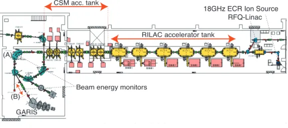
The heavy ion beams of this experiment were distributed by RILAC facility[44].

(21)

5.8 MeV/u by RILAC and charge state multiplier (CSM).

The beam energy was measured by two methods:

1. from the magnetic rigidity of the ions traversing a 90^◦ bending magnet indicated as (A) in Fig. 2.1,

2. by time-of-flight measurement system indicated as (B) in Fig. 2.1.

The accuracy of these systems was±0.2%[49].

18GHz ECR Ion Source RFQ-Linac RILAC accelerator tank

CSM acc. tank

GARIS

Beam energy monitors (B)

(A)

Figure 2.1: Schematic view of the RIKEN heavy ion Linac (RILAC) facility.

2.4 Targets

The series of barrier distribution measurements used three types of targets: ²⁰⁸Pb,

238U and²⁴⁸Cm. The²⁰⁸Pb targets were of a fixed type, while targets of²³⁸U and

248Cm were of a rotating type.

2.4.1

²⁰⁸

Pb Target

The²⁰⁸Pb targets were produced by the vacuum evaporation of metallic²⁰⁸Pb onto 60-µg/cm² carbon backing foils. The thickness of the ²⁰⁸Pb layer deposited was 170 − 230µg/cm²(see Tab. 2.2). To change the beam energy without modifying the RILAC accelerator parameters, aluminum foils were placed in front of the

208Pb target as an energy degrader (see Tab. 2.2).

Figure 2.2 show the target wheel of ²⁰⁸Pb. The targets were mounted at No.

1 - 4, and the energy degrader foils with thicknesses of 0.8, 2.0 and 3.0µm were

(22)

mounted with target No. 2 - 4, respectively. There is a viewer for beam spot tuning at No. 5. The spare targets were mounted at No. 9 - 13 to obtain the balance of the rotating wheel. The target wheel was fixed by adhesive tape. The target positions, it corresponds to change the irradiation target, manually adjusted by the author for every energy points.

Table 2.2: Thickness of energy degraders, backings and target list.

Reaction Energy degraders Carbon backing ²⁰⁸Pb Target (µm) (µg/cm²) (µg/cm²)

None 60 170

48Ca+²⁰⁸Pb 0.8 60 190

2.0 60 220

3.0 60 230

None 60 180

⁵⁰Ti+²⁰⁸Pb 0.8 60 210

2.0 60 190

3.0 60 170

Figure 2.2: The photograph of the²⁰⁸Pb target wheel. The targets were mounted at No. 1, 2, 3 and 4, and the aluminum foils with thicknesses of 0.8, 2.0 and 3.0µm were mounted with target No. 2, 3 and 4. There is a viewer for beam spot tuning at No. 5. The spare targets were mounted at No. 9 - 13 to obtain the balance of the rotating wheel.

(23)

2.4.2

²³⁸

U Target

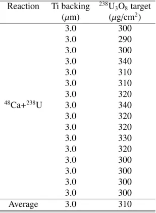
The ²³⁸U3O8 targets were produced by electrodeposition[50] of the material on 3.0-µm-thick Ti backing foils. The 30 cm radius target wheel contained sixteen arc-shaped targets, and it was rotated at 2000 rpm during the beam irradiation. No aluminum degraders were used for the²³⁸U target.

Table 2.3: Thickness of backings and target list for the reaction of⁴⁸Ca+²³⁸U.

Reaction Ti backing ²³⁸U₃O₈target (µm) (µg/cm²)

3.0 300

3.0 290

3.0 300

3.0 340

3.0 310

3.0 320

48Ca+²³⁸U 3.0 340

3.0 320

3.0 330

3.0 320

3.0 300

Average 3.0 310

2.4.3

²⁴⁸

Cm Target

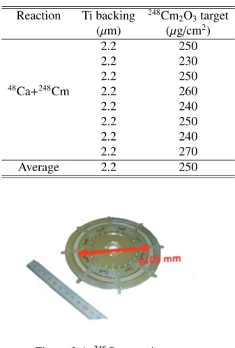
The²⁴⁸Cm₂O₃ targets were produced by electrodeposition[51] of the material on 2.2-µm-thick Ti backing foil for ⁴⁸Ca+²⁴⁸Cm reaction, 2.1-µm-thick Ti backing foil for the reactions ²²Ne+²⁴⁸Cm, ²⁶Mg+²⁴⁸Cm, ³⁰Si+²⁴⁸Cm, ³⁴S+²⁴⁸Cm,

40Ar+²⁴⁸Cm, and⁵⁰Ti+²⁴⁸Cm. The average thickness of the²⁴⁸Cm₂O₃ layer was deposited 250µg/cm² for the reaction of ⁴⁸Ca+²⁴⁸Cm, 450µg/cm² for the other

248Cm reactions. The 10-cm-radius target wheel contained eight arc-shaped targets, and it was rotated at 1000 rpm during the beam irradiation. No aluminum degraders were used with the²⁴⁸Cm target. There was a beam slit (Ta) in front of the²⁴⁸Cm targets (see Fig. 2.5).

(24)

Figure 2.3: ²³⁸U rotating target. This photo was taken from the down stream side of the beam line.²³⁸U targets were deposited by electrodeposition in this side.

Table 2.4: Thickness of backings and target list for the reaction of⁴⁸Ca+²⁴⁸Cm.

Reaction Ti backing ²⁴⁸Cm₂O₃target (µm) (µg/cm²)

2.2 250

2.2 230

2.2 250

48Ca+²⁴⁸Cm 2.2 260

2.2 240

2.2 250

2.2 240

2.2 270

Average 2.2 250

(25)

Table 2.5: Thickness of backings and target list for the reactions of ²²Ne, ²⁶Mg,

30Si,³⁴S,⁴⁰Ar,⁵⁰Ti+²⁴⁸Cm.

Reaction Ti backing ²⁴⁸Cm2O3target (µm) (µg/cm²)

2.1 460

2.1 440

22Ne,²⁶Mg,³⁰Si,³⁴S,⁴⁰Ar,⁵⁰Ti+²⁴⁸Cm 2.1 450

2.1 450

2.1 460

Average 2.1 450

2.5 The gas-filled recoil ion separator GARIS

2.5.1 Overview of GARIS

As shown in Fig. 2.6, GARIS[39, 40] consists of an initial dipole magnet (D1), followed by two quadrupole magnets (Q1) and (Q2), and a final dipole (D2) magnet. The separator was filled with pure helium gas at a pressure of ∼ 120 Pa.

The gas was inserted between D2 and focal-plane detection system, and the gas was discharged by diﬀerential pumping system which is upstream from the rotating target and protects the accelerator. The entrance of the detector chamber at the focal-plane was sealed by 0.5-µm mylar foil to maintain a high-vacuum with pressure below 3.0× 10⁻⁵Torr, as required to prevent the discharge of the MCP detector. The ion optics property of GARIS is shown in the Table 2.6.

Table 2.6: The ion optics property of GARIS Magnification (x) -0.76

Magnification (y) -1.99 Dispersion 0.97 cm/% Acceptance∆θ ± 68 mrad Acceptance∆ϕ ± 57 mrad Acceptance∆Ω 12.2 msr Total length 5.76 m

(26)

Beam slit (Ta)

Beam path

Figure 2.5: The target box for²⁴⁸Cm rotating target.

2.5.2 Beam intensity monitor (45

^◦

elastic monitor)

For the normalization of measured excitation functions using the Rutherford scattering cross section, Rutherford scattering events were measured by a silicon detector (see Fig. 2.7) with an active area of 3.6 × 3.6 mm², mounted either 25 or 142 cm downstream of the target at 45^◦with respect to the beam axis (see Fig. 2.6). The calculated results of Rutherford cross sections in Sec. A.5 indicate the detected events at angles more forward thanθlab= 91^◦follow Rutherford scattering. We can regard the observed elastic scattering atθlab = 45^◦as Rutherford scattering events at every incident energy in this study.

(27)

0 1 2 [m]

He gas region

D2 Q2

Q1 D1

GARIS

Primary beam

Beam intensity monitor Target

Beam stopper (Ta)

Recoiled target-like nuclei Primary beam

Differential pumping Beam slit (Ta)

Figure 2.6: Schematics of GARIS. GARIS consists of an initial dipole magnet (D1), followed by two quadrupole magnets (Q1) and (Q2), and a final dipole (D2) magnet. This figure was taken from Ref. [37].

2.6 Focal plane detectors

The focal plane detectors comprised time-of-flight (ToF) detectors and a 16-strip position sensitive silicon detector (PSD) (see Fig. 2.8).

2.6.1 Time-of-flight detectors

The time-of-flight detectors were used for measurement of time-of-flight of the nuclei at the focal plane. Time-of-flight detectors were constructed of mylar foil, wire grids for making some electric fields, and micro channel plates. The mylar windows were made from 0.5-µm-thickness mylar, and it have an 85-mm diam- eter window coated by 100Å Au and 20-µg/cm² CsI to increase the secondary

(28)

Figure 2.7: The photograph of PIN photodiode. This figure was taken from Ref. [52].

L = 29.5 cm ToF

Targ et-li ke

PSD Strip 0 Strip 15

Figure 2.8: Schematics of the focal plane detector system composed of two time- of-flight detectors and a 16-strip position-sensitive silicon detector (PSD). This figure was taken from Ref. [37].

(29)

electron emission probability. The windows emit the secondary electrons when the heavy-ion pass the mylar windows. The secondary electrons were accelerated by the electric field between mylar foil and wire grid 1, deflected by the electric field between wire grids 2 and 3, amplified by micro channel plates (MCP) and detected by cathode plates. The distance between mylar foils was 295 mm. Since the eﬃciency of the time-of-flight detector was 99% for alpha particles from the

241Am source[53], the target-like events of ²⁰⁸Pb, ²³⁸U and ²⁴⁸Cm should have been detected with closed to the 100%. The full width at half maximum (FWHM) of the timing resolution was 700 ps.

Mylar foil

Micro Channel Plate (MCP) Electron

Heavy ion Wire grid 1

Wire grid 2 Wire grid 3

Cathode plate

Figure 2.9: Schematic view of the time-of-flight detector.

2.6.2 Position sensitive silicon detector (PSD)

The PSD detector was used for measurement of the implantation energy of the nuclei at the focal plane. The PSD detector has an active area of 58×58 mm²and is divided into 16 strips. The thickness of the detector was 300µm. The PSD has position sensitivity only along the vertical axis. Since the PSD was divided to 16 strips, we were able to know the positions for horizontal axis. A precise energy calibration of the PSD strips was performed on the basis of the well-known²⁵⁴No decay lines via the⁴⁸Ca+²⁰⁸Pb reaction.

2.7 Data aquisition system

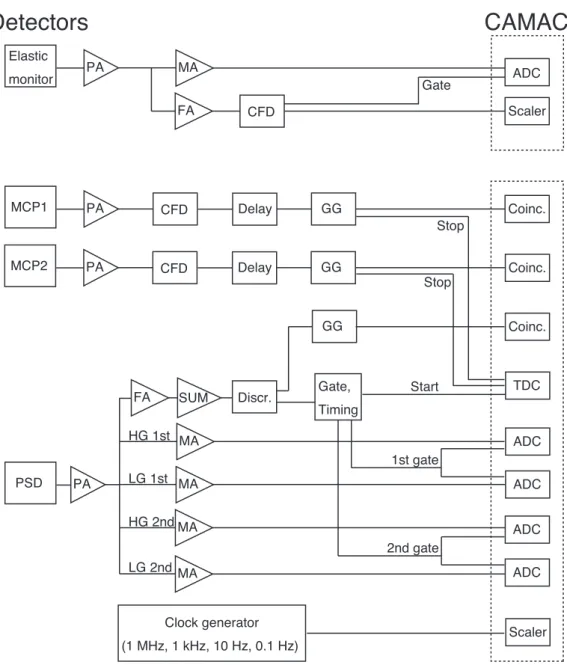
The events data were gathered by CAMAC/NIM system controlled by Linux OS personal computer. Figure 2.10 shows the block chart of the single processing and the data acquisition system. The signals were managed by electronic devices

(30)

indicated in 2.10, and the data were controlled by NaoDAQ program via crate con- troller CC7700. The data acquisition system was started by the signal measured by the PSD. The electronic discriminator level was set to approximately 1 MeV.

The events of our experiment were sorted for each incident energy. Our sort code was written on the basis of the ROOT code[54].

2.7.1 1st-2nd mode

The 1st-2nd DAQ mode was used for the reactions of⁴⁸Ca+²⁰⁸Pb,⁵⁰Ti+²⁰⁸Pb and

48Ca+²⁴⁸Cm. In case of searching the very short-lived nuclei correlation events (∼1 s), the 1st-2nd DAQ mode is used not to miss the DAQ for the very short-lived event which just after the preceding event. Figure 2.11 shows the time window for the 2nd gate. In case the time diﬀerence which between 1st event and 2nd event is 5−255µs, the 2nd event is observed by the 2nd gate.

The 2nd gate event was not used as an event of the QE scattering event in this barrier distribution study. The 1st-2nd DAQ mode was used for the reactions

48Ca+²⁰⁸Pb, ⁵⁰Ti+²⁰⁸Pb and ⁴⁸Ca+²⁴⁸Cm due to the machine time management with evaporation residue measurement. The dead time was revised to take into account for the diﬀerence of the dead time. The dead time was 310 µs in case of the only 1st gate event. The dead time was 480 µsin case of the 1st-2nd gate event.

The 1st-2nd mode was not used for the reactions²²Ne+²⁴⁸Cm, ²⁶Mg+²⁴⁸Cm,

30Si+²⁴⁸Cm,³⁴S+²⁴⁸Cm,⁴⁰Ar+²⁴⁸Cm,⁵⁰Ti+²⁴⁸Cm,⁴⁸Ca+²³⁸U.

2.7.2 Dead time

It takes 310µs to gather the data if only the 1st gate is used in the data acquisition (DAQ) system. The dead time is 3.1% in case of 100 counting per second at the focal plane detectors. The data were corrected for dead time. The dead time should be decreased as much as possible. The counting ratio at the focal plane detectors was checked and the beam intensity adjusted so as to maintain 100 - 200 counts per second at each energy setting.

(31)

Elastic

monitor PA MA

FA CFD

Gate ADC

Scaler

MCP1 PA CFD Delay GG Coinc.

MCP2 PA CFD Delay GG Coinc.

Coinc.

TDC Stop

Stop GG

PSD PA MA

MA SUM MA

MA HG 1st

FA

LG 1st HG 2nd

LG 2nd

Discr. Gate, Timing

Clock generator (1 MHz, 1 kHz, 10 Hz, 0.1 Hz)

ADC ADC ADC ADC 1st gate

2nd gate Start

Scaler

Detectors CAMAC

Figure 2.10: Block chart of the data acquisition system. PA : Pre-Amplifier, MA : Main-Amplifier, FA : Fast Amplifier, CFD : Constant Fraction Discriminator, Delay : Digital delay box, GG : Gate and delay Generator, Discr. : Discriminator, ADC : Analog to Digital Converter, Coinc. : Coincidence Register, TDC : Time to Digital Converter

(32)

Time OFF

ON

1st gate 2nd gate

Event

5 μs 35 μs

2nd gate open 250 μs

[μs]

0 5 255 290

Figure 2.11: Time window for the 2nd gate.

(33)

Chapter 3 Data Analysis and Results

Data analysis and results are described in this chapter. The particle identification, separation of deep-inelastic scattering events, transmission eﬃciency, analysis of 45^◦elastic monitor and experimental barrier distributions will be explained in this chapter.

3.1 Particle Identification

3.1.1 ToF-E matrix

The analysis procedure of the⁴⁸Ca+²⁴⁸Cm reaction, as shown in Fig. 3.1, should serve as an example for the analysis of all reactions described in tis section. Fig- ure 3.1 shows two-dimensional (2D) plots of the content of the ToF-E matrix for the reaction ⁴⁸Ca+²⁴⁸Cm as described in Ref. [37]. From the expected energy calculations, such as the two body reaction, energy loss calculation in target, mylar windows, helium gas in GARIS, the events in the 2D plots were classified as follows:

• ²⁴⁸Cm target-like events,

• ¹⁸¹Ta-like events sputtered from the stopper by an impinging beam,

• ¹⁸¹Ta-like events sputtered from the slits by an impinging beam,

• ⁴⁸Ca beam-like events.

The ¹⁸¹Ta (beam slit) events were not observed in case of ²⁰⁸Pb and ²³⁸U target reactions, because there was no beam slit.

(34)

0 5 10 15 20 25 30

0 20 40 60 80 100 120 140

×

10 0 ×

10 20 30 40 50 60 70 80 90 100

Time-of-Flight [ns]

0 10 20 30 40 50 60 70 80 90 E_c.m. = 174.8 MeV

10 0 ×

10 20 30 40 50 60 70 80 90

0 10 20 30 40 50 60 70 80 E_c.m. = 186.3 MeV 90

10 0 ×

10 20 30 40 50 60 70 80 90

0 50 100 150 200 250 300 350 Ec.m. = 208.2 MeV 400

0 20 40 60 80 100 120

10

× Energy [MeV]

0 10 20 30 40 50 60 70 80 90

0 5 10 15 20 25 30 35 40 45 E_c.m. = 221.5 MeV

Target-like

181Ta (Beam slit) Beam-like

181Ta (Beam stopper)

30 32 34 36 38 40 42 44 46 48 50

50 60 70 80 90 30 50 60 70 80 90 32

34 36 38 40 42 44 46 48 50

Energy [MeV]

Time-of-Flight [ns]

E_c.m. = 221.5 MeV E_c.m. = 208.2 MeV

(a)

(b)

181Ta (Beam slit) Target-like 48Ca +²⁴⁸Cm

Figure 3.1: (a) Two-dimensional plots of ToF vs E. The vertical axis shows the

(35)

3.1.2 Estimation of the mass

As shown in Fig. 3.1, ¹⁸¹Ta-like events resulting from beam impinging the slits were observed to be commingled with²⁴⁸Cm target-like events. To more clearly separate these events required an eﬀort to estimate masses from the time-of-flight and energy measurements.

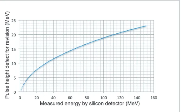
3.1.3 Pulse height defect

Electron and hole pairs are made in proportion to the kinetic energy of the implanted nucleus when lighter nuclei are implanted in a silicon detector. The kinetic energy of the implanted nuclei can be measured due to the electrons and holes moving to electric plates. In the case of heavy nuclei, the kinetic energy is released only within a very narrow range, then, some electrons and holes are combined again by ion recombination. The pulse height is artificially diminished.

This phenomenon is called the “pulse height defect”.

The eﬀect can be corrected by the method from the Ref. [55]. The following parameters, such as, the atomic number and mass of implanted nucleus Z₁ and M1, the atomic number and mass of detector materialZ2 and M2, Bohr radiusa0

were used to define the Kaufman constantk,

k= 0.8853a0(Z₁^2/3+Z₂^2/3)⁻¹^/²M2

Z₁Z₂e²(M₁+M₂) . (3.1) For example, the Kaufman constant isk = 0.5208 in case of²³⁸U implanted in the silicon detector. The parameterϵis defined as

ϵ =kE. (3.2)

By using thisϵ, the pulse height defect∆ϵis calculated as

∆ϵ(ϵ)= 6ϵ

ϵ+8 + A

1+525ϵ⁻¹^.⁴⁰⁷. (3.3) A is a free parameter ranging from 13 to 15. In this time, A = 14 is employed as it yields the maximally parsimonious experimental results. For example, the

∆ϵ = 16 MeV for E= 70 MeV of the combination of²⁴⁸Cm and silicon detector (see Fig. 3.2).

The variation of∆ϵ resulting from variation of the free parameterAis shown in Table 3.1. As the free parameterAdoes not significantly aﬀect the value of∆ϵ, the choice ofAsimilarly does not impact the particle identification.

(36)

Measured energy by silicon detector (MeV)

Pulse height defect for revision (MeV)

Figure 3.2: Calculated pulse height defect for combination of ²⁴⁸Cm and silicon detector based on Ref. [55].

Table 3.1: Calculated pulse height defect for combination of ²³⁸U and silicon detector based on Ref. [55] with changing the free parameter AbetweenA = 13 andA=15 at E =70 MeV.

A ∆ϵ(MeV)

13 15.0

14 15.5

15 16.0

3.1.4 Energy loss in mylar window

The time-of-flight between mylar 1 and mylar 2, indicated in Fig. 3.3, was gathered. The energyE₂indicated in Fig. 3.3 should be derived to estimate the correct mass for passing nuclei. The energy corresponding toE3in Fig. 3.3 was extracted by using the measured energy from the PSD and the correction of pulse height defect. To obtainE₂, the energy was modified using the following three-step procedure:

1. TheE₂-value was estimated by assuming all events were²⁴⁸Cm by the time- of-flight information,

(37)

3. TheE₂-value was derived by the sum of the calculated energy loss at mylar foil 2 andE3.

The value ofE2 was extracted from the measured energy at PSD and time-of- flight informations by this procedures.

E₁ E₂ E₃

Mylar 1 Mylar 2

Time-of-flight detectors PSD

Figure 3.3: Explanation for energy loss in mylar foils.

3.1.5 Estimated mass

The mass of passing nuclei was estimated from the measured time-of-flight and calculated energy based on measured energy. The mass-like M_like of nuclei was calculated by using the E2 in Fig. 3.3 and time-of-flight TToF measured by ToF detectors and the flight pass of ToF detectorL_ToF(= 29.5 cm),

Mlike =2EToF

T_ToF²

L²_ToF. (3.4)

Figure (a) in Fig. 3.4 show the 2D plots of the time-of-flight vs. M_like (ToF- M_like). The events were clearly assigned using the above calculation to be:

• ²⁴⁸Cm target-like events,

• ¹⁸¹Ta-like sputtered from the stopper by an impinging beam,

• ¹⁸¹Ta-like sputtered from the slits by an impinging beam,

• ⁴⁸Ca beam-like events.

For lighter nuclei, such as⁴⁸Ca and¹⁸¹Ta, theM_likevalues were overestimated, because the revision parameters were optimized for²⁴⁸Cm target-like events. Nev- ertheless, this analysis allowed for the clear identification of the events.

(38)

Figure 3.4 (b) and (c) show a zoom-in of the red square region in Fig. 3.4 (a). A valley between the¹⁸¹Ta-like (beam slit) components and²⁴⁸Cm target-like components was clearly observed in the plot, allowing for unambiguous determination of the²⁴⁸Cm target-like events. The target-like events gate for every experimental energy setting was defined from such figures.

3.2 Separation of deep-inelastic scattering events

The treatment of deep-inelastic (DI) scattering events is introduced in this section.

The previous experiments of DI events are also introduced. The observed DI events were displayed and the upper limit for DI events were derived.

3.2.1 Previous methods for the treatment of the deep-inelastic scattering events

In a previous work from Mitsuokaet al.[36], DI scattering events were not able to be separated from QE scattering events, because they did not use a separator such as GARIS. However, they were able to observe the QE and DI events without any separation. They applied two techniques to their analysis:

• set the borderline at − Q = 20 MeV following the study from Rehm et al.[56],

• comparison with the simulation results from the Monte Carlo reaction simulation code LINDA[57].

3.2.2 Upper Limit for Contaminated Deep-inelastic Events

It is diﬃcult to distinguish the QE event from the DI event. The main part of DI event was measured by changing the magnetic rigidity parameter of GARIS. The upper limits of the DI events were estimated from the main part of the DI events.

The parameter is not suitable for DI event when the magnetic rigidity parameter is set for QE event. The DI events should be decreased compared to the case of the optimum one. The upper limit for DI event was estimated by this logic.

Two dimensional plots of ToF-E and ToF-M

The target-like events were divided into QE and DI event using the observed data to estimate the DI components. Left side panels of Fig. 3.6 shows a two-

(39)

0 50 100 150 200 250 300 350 400

Mass-like [u]

0 10 20 30 40 50 60 70 80 90 100

Time-of-Flight [ns]

0 20 40 60 80 100

Beam-like

Target-like

181Ta (Beam slit)

181Ta (Beam stopper)

48Ca+²⁴⁸Cm Ec.m. = 219.8 MeV

200 210 220 230 240 250 260 270 280

26 28 30 32 34 36 38 40 42 44 46

0 20 40 60 80 100

Time-of-Flight [ns]

Target-like

181Ta (Beam slit)

Mass-like [u]

200210 220230

240250 260270

Mass[u] 280 ₂₆ ²⁸ ³⁰ ³²

34 36 38 40 42

Time-of-Flight [ns]

0 20 40 60 80 100 120

Counts

(a)

(b)

(c)

181Ta (Beam slit)

Target-like

Figure 3.4: Graphical explanation of how to separate target-like event and the

181Ta event from beam slit.

(40)

70

Zn+

²⁰⁸

Pb

Figure 3.5: Measured energy spectrum at θ = 172^◦ in ⁷⁰Zn+²⁰⁸Pb at Ec.m. = 254.9 MeV. This figure is taken from Ref.[36]. They tried to repro- duce the shape of the DI component by using the Monte Carlo reaction simulation code LINDA[57]. σMassandσTKEis the input parameter of the simulation code.

reaction⁴⁰Ar+²⁴⁸Cm similarly to Fig. 3.1. The two diﬀerent magnetic rigidity settings of the GARIS for every incident energy is displayed in Fig. 3.6. The energy E_c_._m_.and the magnetic rigidity settings was written in the figures.

Some 2D plots of the content of the ToF vs. Mass-like (ToF-M) following the procedures in Sec. 3.1.5, and displayed in center panels of Fig. 3.6. The magnetic rigidity setting is same as just left side panels. To discuss the behavior of DI and QE events, the red rectangular regions were used as the gate for target-like component (target-like gate).

Right side panels of the Fig. 3.6 show some energy spectra of the events which were gathered by target-like gate, and the energy Ec.m. and the magnetic rigidity setting is same as just left side panels. The valleys were observed following figures:

• energy=18 MeV forEc.m.= 154.5 MeV with 1.668 Tm,

• energy=26 MeV forE_c_._m_.= 181.2 MeV with 1.632 Tm,

• energy=33 MeV forE_c.m.= 193.7 MeV with 1.596 Tm.

From the comparison with Figs. 3.6 and 3.5 from the previous work in Mit- suoka et al.[36], the low energy side hump shown in the right side panels of the E_c.m. = 154.5 MeV 1.668 Tm, E_c.m. = 181.2 MeV 1.632 Tm and E_c.m. = 193.7 MeV 1.596 Tm in the Fig. 3.6 is assigned as DI components.

Study of Fusion Barrier Distributions from Quasielastic Scattering Cross Sections

超重核合成に向けた準弾性散乱による融合障壁分布 の研究

Study of Fusion Barrier Distributions from Quasielastic Scattering Cross Sections

towards Superheavy Nuclei Synthesis

Taiki Tanaka

Department of Physics, Kyushu University

February 11, 2019

Abstract

Contents

Chapter 1 Introduction

1.1 History of the new elements

1.2 Superheavy elements

1.2.1 Liquid drop model

1.2.2 Shell model and macroscopic-microscopic model

1.2.3 Quantum many body system

1.2.4 Frontier of the nuclei

1.2.5 Importance for optimum incident energy

E

(MeV) σ

( μ b )

1.2.6 How to solve the problem of optimum incident energy

1.3 Fusion barrier distribution

1.3.1 Previous works for barrier distribution studies and su- perheavy nuclei synsthesis

1.3.2 Weak points in previous works

1.4 Thesis objectives

1.4.1 Purpose of this thesis

1.4.2 New method of barrier distribution measurement

1.4.3 Fusion dynamics for synthesizing superheavy nuclei

1.4.4 Systematics of hot fusion reactions

1.5 Contributions

Chapter 2 Experiment

2.1 Overview of the Experiment

2.2 Beam

2.2.1 Ions

2.2.2 Beam intensity and attenuators

2.3 Accelerator

2.4 Targets

2.4.1

Pb Target

2.4.2

U Target

2.4.3

Cm Target

2.5 The gas-filled recoil ion separator GARIS

2.5.1 Overview of GARIS

2.5.2 Beam intensity monitor (45

elastic monitor)

0 1 2 [m]

D2 Q2

Q1 D1

GARIS

2.6 Focal plane detectors

2.6.1 Time-of-flight detectors

L = 29.5 cm ToF

Targ et-li ke

PSD Strip 0 Strip 15

2.6.2 Position sensitive silicon detector (PSD)

2.7 Data aquisition system

2.7.1 1st-2nd mode

2.7.2 Dead time

Detectors CAMAC

Time OFF

ON

1st gate 2nd gate

Event

Chapter 3

Data Analysis and Results

3.1 Particle Identification

3.1.1 ToF-E matrix

3.1.2 Estimation of the mass

3.1.3 Pulse height defect

3.1.4 Energy loss in mylar window

3.1.5 Estimated mass

3.2 Separation of deep-inelastic scattering events

3.2.1 Previous methods for the treatment of the deep-inelastic scattering events

3.2.2 Upper Limit for Contaminated Deep-inelastic Events

Zn+

Pb

超重核合成に向けた準弾性散乱による融合障壁分布の研究