欠陥を有するカーボンナノチューブの熱輸送特性

九州大学学術情報リポジトリ

Kyushu University Institutional Repository

欠陥を有するカーボンナノチューブの熱輸送特性

林, 浩之

https://doi.org/10.15017/1441239

出版情報：Kyushu University, 2013, 博士（工学）, 課程博士 バージョン：

権利関係：Fulltext available.

欠陥を有するカーボンナノチューブ

の熱輸送特性

博士（工学） 学位論文

九州大学大学院 工学府航空宇宙工学専攻

林 浩之

平成 26 年 1 月

目次

第

章 序論

概要

カーボンナノチューブ（

）の熱輸送特性

初期の実験的研究と多層

（

）の異方性

直接通電による熱伝導率計測

ラマン分光による熱伝導率計測

長さ依存性

欠陥依存性

単層

（

）の分子構造とカイラリティ依存性

熱整流作用

グラフェンの熱輸送特性

研究目的

論文の構成

第

章 熱処理によって欠陥を導入した

の熱輸送特性

概要

熱伝導率計測の原理

キャリブレーション

サンプルの計測

センサの作製方法

実験系

計測装置および装置の設定

熱起電力による計測誤差と対策

熱処理を行っていない

の熱伝導率計測

キャリブレーション

MWNT

の計測

熱酸化による欠陥の導入

熱処理の方法

加熱温度の決定

TEM

観察による欠陥の評価

熱伝導率の計測結果

考察

異方性を考慮した熱伝導シミュレーション

層間のギャップの影響 ... 57

まとめ ... 59

第

章 集束イオンビームによって欠陥 を導入した

の熱輸送特性 ... 60 概要 ... 60

集束イオンビームによる欠陥の導入 ... 61

照射条件 ... 61

TEM

観察による欠陥の評価 ... 62

実験系 ... 66

熱伝導率の計測結果 ... 67

考察 ... 68

拡散的な熱伝導モデル ... 68

準弾道的な熱伝導モデル ... 71

異なる長さの

が混在している場合 ... 75

まとめ ... 78

第

章 欠陥の不均一分布による熱整流作用 に関する数値解析 ... 79 概要 ... 79

欠陥が不均一に分布した

を対象とした解析 ... 79

計算手法 ... 79

計算結果 ... 90

考察 ... 92

一次元格子モデルを用いた解析 ... 96

計算手法 ... 97

計算結果 ... 101

考察 ... 102

まとめ ... 106

第

章

の熱伝導率計測手法の開発 ... 107 概要 ... 107

熱伝導率計測の原理 ... 107

センサの製作方法 ... 109

SWNT

の合成およびブリッジ構造の実現 ... 112

ラマン分光による

の評価 ... 114

原理 ... 114

SWNT

のラマンスペクトルの特徴 ... 114

ラマン散乱の共鳴効果 ... 115

分析結果 ... 116

5.5.4

高解像度

による

の評価 ... 120

5.6 SWNT

の切断 ... 122

5.7

実験系 ... 124

5.8

実験結果 ... 125

5.9

考察 ... 127

5.10

まとめ ... 129

5.11

第

章 総括 ... 130

Appendix

両端

の

の熱輸送特性の評価 ... 132

参考文献 ... 138

謝辞 ... 150

List of figures

Figure 1.1 Gaphene-based nanomaterials: SWNT and MWNT. [9] ... 1

Figure 1.2 Anisotropy of thermal conductivity of MWNTs. [9] ... 3

Figure 1.3 (a) Schematic view of heat conduction in a large-diameter MWNT. (b) Thermal conductivity dependence on diameter reported by Fujii et al. [16] and Yang et al. [17] ... 3

Figure 1.4 Thermal conductivity of a shorter SWNT decreases due to phonon scattering at nanotube end. ... 8

Figure 1.5 (a) Upper schematic shows a CNT with various-type defects. Lower schematic shows the representation of single vacancy, double vacancy, and Stone–Wales type defects. (b) Thermal conductivities of a SWNT are plotted as a function of defect concentration.[67] ... 9

Figure 1.6 Illustration diagram of molecular structure of a SWNT. ... 10

Figure 1.7 The chirality and structure of SWNT. Illustration shows edge strutcture of (a) chirality (10,0), (b) chirality (5,5), and (c) chirality (4,6). [9] ... 11

Figure 1.8 (a) Schematic description of mass-deposited nanotube and (b) SEM image of a CNT after deposition of experimentaly obtained solid state thermal rectifier. [84] (c) Schematic view of vacancy defect. (d) Calculation model of SWNT with vacancy defects only in half region of the SWNT.[86] Red arrows in (b) and (d) show direction where heat flows predominantly. ... 14

Figure 2.1 Schematic view of heat conduction in (a) a pristine MWNT and (b) a MWNT with a defect which covers whole circumference of the MWNT. [76] ... 19

Figure 2.2 Schematic views of T-type sensor (a) before nanotube attached and (b) after nanotube attached. ... 20

Figure 2.3 SEM image of Pt hotfilm suspended between heatsinks, recorded by tilting the sample 70°. ... 27

Figure 2.4 Schematics of fabrication process of a sensor. ... 29

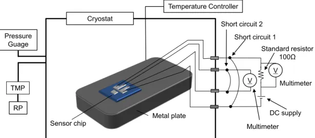
Figure 2.5 Schematic of experimental setup. ... 31

Figure 2.6 Picture of a sensor chip on the metal plate with interconnections. ... 31

Figure 2.7 Schematic of condition where the thermoelectric power is generated. ... 33

Figure 2.8 Effect of offset voltage. ... 33

Figure 2.9 Removing the offset voltage using current reversal method. ... 34

Figure 2.10 Comparison of normal and current reversal method of (a) volt-ampere characteristics and (b) resistance-power characteristics of hotfilm. ... 34 Figure 2.11 Resistance-heating power characteristics of a hotfilm when temperature of heatsink

is 300 K. ... 35

Figure 2.12 Resistance change divided by heating power ΔR/P of a hotfilm vs. temperature of heatsink T0. ... 37

Figure 2.13 Resistance under no heating condition R(0) of a hotfilm vs. temperature of heatsink T0. ... 37

Figure 2.14 Temperature coefficient of resistance per unit resistance β of a hotfilm vs. temperature of heatsink T0. ... 38

Figure 2.15 Thermal conductivity of a hotfilm vs. temperature of heatsink. ... 38

Figure 2.16 SEM image of a T-type sensor with a suspended MWNT between a Pt hotfilm and a heatsink. ... 39

Figure 2.17 TEM image of a pristine MWNT. ... 40

Figure 2.18 Resistance-heating power characteristics of a hotfilm with MWNT (circle plots) and without MWNT (diamond plots) when temperature of heatsink is 300 K. ... 41

Figure 2.19 Resistance change divided by heating power ΔR/P of a hotfilm with MWNT (circle plots) and without MWNT (diamond plots) vs. temperature of heatsink T0. ... 42

Figure 2.20 Temperature coefficient of resistance per unit resistance β of a hotfilm with MWNT (circle plots) and without MWNT (diamond plots) vs. temperature of heatsink T0. ... 42

Figure 2.21 Schematics of heating treatment procedure. ... 43

Figure 2.22 SEM image of MWNTs on Si substrate before heat treatment. ... 45

Figure 2.23 SEM image of Si substrate after heat treatment at 500 °C. ... 45

Figure 2.24 TEM images of outer shell defects in MWNT. (a) Defect covers the whole circumference and (b) confined defect in which an area 50 nm × 50 nm of the outer shell is lost. ... 46

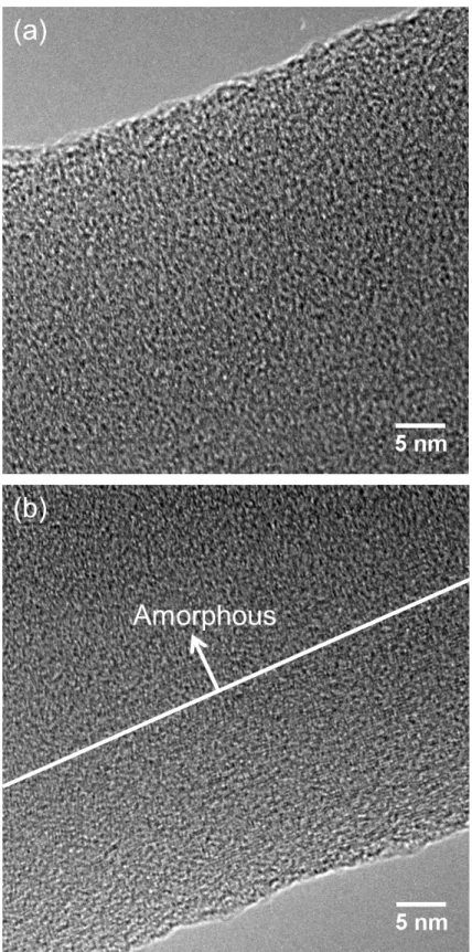
Figure 2.25 High magnificationTEM images of outer shells of not-defective parts of (a) a MWNT after heat treatment (b) a MWNT without heat treatment. ... 47

Figure 2.26 Positions of defects are indicated in a SEM image of a MWNT on TEM grid. Red lines show positions of two large defects which covers the whole circumference of MWNT. TEM images show shape of defects. Scale bar in TEM images show 50 µm. ... 48

Figure 2.27 Thermal conductivities of MWNT with whole circumferential defects (square plots), MWNT with only confined defects (triangle plots), pristine MWNT (circle plots).51 Figure 2.28 Schematic of simulation procedure. ... 53

Figure 2.29 Schematic view of definition of the coordinate where the application surface of adiabatic boundary conditions is shown as thick line. ... 55 Figure 2.30 Temperature distribution obtained using kin = 1800 W/m·K and k_out = 0.05 W/m·K from (a) model of pristine MWNT and (b) model of MWNT with whole circumference

defects, respectively. ... 56

Figure 2.31 TEM images of a pristine MWNT (a) section showing normal structure of graphitic shells and (b) section showing gaps between shells. The dashed lines mark the inner diameter of the MWNT. ... 58

Figure 3.1 (a) Schematic showing the the Ga⁺ ion beam irradiation experiment. (b) A SEM image of the thermal conductance test fixture, with a MWNT before FIB irradiation. The lines indicate FIB irradiation positions, with numbers denoting the nth irradiation. The 1st position is 1/2 way from the heat sink to the sensor. The 2nd and 3rd positions are 1/4 and 3/4 of the way, respectively. The 4th–7th positions are at 1/4 increments from 1/8 to 7/8, respectively. The 8th–15th positions are at 1/8 increments from 1/16 to 15/16, respectively. (c) SEM image of the FIB irradiation traces on the substrate. ... 60

Figure 3.2 Schematic view of the shape of the amorphous part with squares indicating the position where TEM images of Figure 3.3 (a), (b) and Figure 3.4 are obtained. ... 63

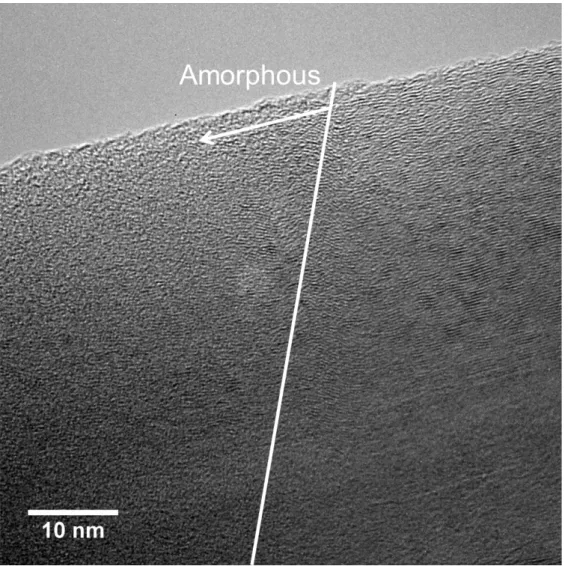
Figure 3.3 TEM images of the FIB-irradiated MWNT: (a) upper part of the MWNT irradiated directly and (b) lower part of the MWNT showing partially-remained structure of graphitic shells. These images were recorded by tilting the sample 70° toward the FIB irradiation direction. ... 64

Figure 3.4 TEM images of the FIB-irradiated MWNT obtained at the boundary of amorphization. ... 65

Figure 3.5 Schematic diagram of a cross-section of the amorphized MWNT. ... 65

Figure 3.6 Schematic of experimental setup in Versa 3D. ... 66

Figure 3.7 Picture of a sensor chip on Cu base with interconnections. ... 66

Figure 3.8 Measured thermal conductance at 300 K as a function of irradiation time. 0th irradiation indicates pristine MWNT before irradiated. Inset shows the temperature dependence of thermal conductance of pristine, 1st, 3rd, 7th, and 15th irradiated nanotubes at 260–320 K. ... 68

Figure 3.9 Schematic of thermal resistance change due to first irradiation on the assumption of diffusive thermal transport. ... 69

Figure 3.10 Thermal conductance measured (diamond plots) and calculated using the diffusive conduction model with gdefect−1 = 0.00037 K/nW (upper blue dotted line) and gdefect−1 = 0.00095 K/nW (lower red dotted line), at 300 K as a function of irradiation time. ... 70

Figure 3.11 Schematic of thermal resistance change due to first irradiation on the assumption of quasi ballistic thermal transport. ... 71 Figure 3.12 Thermal conductivity as a function of length ln of equally-divided MWNTs calculated using g ⁻¹ of 0, 0.00016, 0.00027, and 0.00034 K/nW are indicated by the

diamond plots, solid line, dashed-dotted line, and dotted line, respectively. ... 73

Figure 3.13 Schematic of three assumptions used to describe heat transfer phenomena when the different length of MWNT are connected. ... 76

Figure 3.14 Measured thermal conductance with error bars (diamond plots), and conductance calculated from the first (solid), second (dotted), and third (dashed) assumptions. ... 78

Figure 4.1 Simulation models of (5,5) SWNT: (a) to apply Langevin method and (b) to apply Nosé-Hoover method. ... 81

Figure 4.2 Schematic view of vacancy defect. ... 81

Figure 4.3 Relative position of mass points. ... 83

Figure 4.4 Calculation of the temperature distribution in the axial direction of SWNT. ... 86

Figure 4.5 Tempareture distribution in SWNT axial direction of (a) model of Langevin method and (b) model of Nosé-Hoover method． ... 91

Figure 4.6 Phonon DOS: (a) case of heat flow from pristine part to defective part and (b) case of heat flow from defective part to the pristine part. ... 95

Figure 4.7 Phonon DOS obtained from atoms near vacancy. ... 96

Figure 4.8 1D model for simulating the atoms near defects of SWNT. ... 97

Figure 4.9 (a) Fluctuation of instantaneous heat flux averaged every 5×10³ dimensionless time. (b)Temporal average of the dimensionless heat flux. Two dot-lines show ±0.5% of final value. ... 100

Figure 4.10 Temperature profile of 1D chain model using kR = 0.1 (dashed line), 0.01 (solid line). ... 101

Figure 4.11 Phonon spectra for kR = 0.1, |Δ| = 0.7, and dimensionless temperature is 1. (a) shows phonon spectra for Δ > 0. (b) shows phonon spectra for Δ < 0. ... 103

Figure 5.1 Temperature distribution in SWNT. ... 107

Figure 5.2 Schematics of fabrication process of electrode with trench for four probe method.112 Figure 5.3 Procedure of synthesis of SWNTs on the four-terminal electrodes. ... 113

Figure 5.4 Kataura plot. ... 115

Figure 5.5 Raman signals of RBM mode obtained by using the 532nm-wavelength laser. ... 116

Figure 5.6 Kataura plot with the wavelength of the RBM mode obtained by using the 532 nm-wavelength laser light. ... 117

Figure 5.7 Raman signals of RBM mode obtained by using the 633nm-wavelength laser. ... 118

Figure 5.8 Kataura plot with the wavelength of the RBM mode obtained by using the 633 nm-wavelength laser light. ... 118

Figure 5.9 Raman signals of RBM mode obtained by using the 785-wavelength laser. ... 119

Figure 5.10 Kataura plot with the wavelength of the RBM mode obtained by using the 785 nm-wavelength laser light. ... 119

Figure 5.11 SEM images of SWNT suspended between electrode with (a) no tilt and (b) tilting sample (30°). The SWNT contacts with the substrate. ... 120 Figure 5.12 SEM images of SWNT suspended between electrode with (a) no tilt and (b) tilting sample (30°). The SWNT does not contact with the substrate. ... 121 Figure 5.13 SEM images of a SWNT (a) before cutting and (b) after cutting. ... 122 Figure 5.14 Raman signal of G band and D band due to the laser light wavelength of 785nm obtained from (16,7) nanotube. ... 123 Figure 5.15 (a) Schematic of experimental setup and circuit diagram. (b) Enlarged view of the substrate. (c) SEM image of SWNT suspended beteween electrodes. ... 124 Figure 5.16 The current-voltage curve at each heat sink temperature ... 125 Figure 5.17 The resistance-heatingpower curve at each heat sink temperature. ... 125 Figure 5.18Changes that appeared in each measurement to the resistance vs. heating power curve at the heat sink temperature 300K ... 126 Figure 5.19 Circuit diagram of four-probe method. ... 127 Figure 5.20 Schematic view of SWNTs remain between voltage and current electrodes. ... 128 Figure 5.21 Circuit diagram contains current path between voltage and current electrodes. ... 128

List of Tables

Table 1.1 Thermal conductivities of individual carbon nanotubes at room temperature. ... 6

Table 1.2 Measured thermal conductivities of graphene at room temperature. ... 16

Table 2.1 Positions and dimensions of defects of two measured MWNTs. ... 49

Table 2.2 Characteristics of measured MWNTs. ... 50

Table 3.1 Conditions of the FIB irradiation. ... 61

Table 3.2 Thermal conductivity contribution of phonons with a certain free path range. ... 74

Table 4.1 Parameters of Brenner potential. ... 84

Table 4.2 Simulatin results of model (a) using Langevin method. ... 92

Table 4.3 Simulatin results of model (b) using Nosé-Hoover method. ... 92

Table 4.4 Obtained heat flow and calculated thermal rectification rates. ... 102

序論 第 1 章

概要

カーボンナノチューブ（carbon nanotube; CNT）は一層もしくは多層のグラフェンを繋ぎ 目無く円筒状に丸めた構造を有し，一層の物を単層

SWNT），多層の物を多層CNT（multi-walled carbon nanotube; MWNT）と呼ぶ（Figure 1.1）．

端が丸く閉じているか開いてグラフェンのエッジがむき出しになっているかで

open end

と区別される[1]．

の直径は

から太いもので

程度，

は

から

を超える程度で，長さはそれぞれ

から数

の物まで存在する．したが

って直径は

オーダーでありながら長さはマクロなスケールに達し得る特異な材料であ る．さらに，弾性係数は

で既存のあらゆるファイバーの

倍 を超え[2]，熱伝導率は室温でダイヤモンドを超える

（金や銅配線は

程度）に達し[4]，電子移動度も

を超えシリコンの

倍[5]であり，優れた性質を有する．近年では世界の

メーカの年間生産力は数千

にも及び[6]，

トランジスタを用いた計算機が

誌に紹介される[7, 8]等，その工業 的・学術的な関心は高まり続けている．

本章では，CNT の熱輸送特性を既存の研究成果と併せて解説した後，CNT の分子構造と 電気的特性，熱整流作用，グラフェンの熱的特性について概説し，本論文の目的，構成を 述べる．

  Figure 1.1 Gaphene-based nanomaterials: SWNT and MWNT. [9]

Graphene

Single-walled carbon nanotube (SWNT)

Multi-walled carbon nanotube (MWNT)

カーボンナノチューブ（CNT）の熱輸送特性

CNT

の高い熱伝導率は強力な

混成軌道による結合と繋ぎ目の無い分子構造のための 長いフォノン平均自由行程（phonon mean free path; PMFP）に由来する．この高い熱伝導率 のため電子機器や導線として利用した際の高い排熱効果，ポリマーや金属の複合材料のフ ィラー材として用いることで複合材料の熱伝導率や電流容量を向上させる

の利用が期待され熱輸送特性の解明が求められる．本節では既存の研究成果を紹介する．

初期の実験的研究と多層

SWNT

マットを用いた最初期の計測では，

と低い熱伝導率が得られている[13]．

これは計測に用いた試料が複数の

が寄り集まったマットであるためにナノチューブ

‐ナノチューブ間の接触熱抵抗の影響が大きく現れているためである．その後，ピエゾ駆 動のマニピュレータ・走査型電子顕微鏡（scanning electron microscope; SEM） ・EBID （electron

beam-induced deposition）[14]といったナノテクノロジーを組み合わせてMWNT

をハンドリ

ングすることで，単一の

の熱伝導率計測が行われた．Kim らは

mechanical systems

（MEMS）技術によって梁で真空中に懸架された窒化ケイ素薄膜上に白金

抵抗体をパターニングしたものを一対作製し，その間に架橋した

内に発生した熱流 を検知することで熱伝導率を計測した[15]．

らもヒータ兼測温抵抗体として働く白金ホ ットフィルムを用いた

型一体型センサを用いることで計測に成功している[16]．これらの 単一の

を用いた信頼性の高い計測によって直径

程度の

の熱伝導率は

室温で

にも及ぶということが明らかになった．

更に

らはこの手法を用いて直径の異なる

の熱伝導率を計測することで直径

の大きな

ほど熱伝導率が低くなることを示した．同様の傾向が

らによっても 報告されている[17]．MWNT においては

に示すように

結合による層内方向の 高い熱伝導率と分子間力による層間方向の低い熱伝導率が複合している（熱伝導率の異方 性）．さらに，Figure 1.3 (a)のように，計測の際にセンサやヒータと接しているのは

の外層であるため，直径が大きいほど内層に熱が伝わらなくなる．そのため直径が大きい ほど内層の熱輸送への寄与が小さくなり，熱伝導率の直径依存性が生じる（Figure 1.3 (b)）．

このように，熱伝導率の異方性は

全体の熱輸送量に大きく影響する[15–17]．しかし

ながら，この異方性に関して定量的なデータは未だ存在せず，CNT の熱輸送特性における

未踏領域の

つと言える．

  Figure 1.2 Anisotropy of thermal conductivity of MWNTs. [9]

  Figure 1.3 (a) Schematic view of heat conduction in a large-diameter MWNT. (b) Thermal conductivity dependence on diameter reported by Fujii et al. [16] and Yang et al. [17]

単一の

を用いた最初の計測は

ら[18]によって[15]のデバイスを用いて行われた．

SWNT

のハンドリングは困難なため，この計測は

を合成する

法[19]において合 成の起点となる触媒をセンサ上に配置することで

が

つのセンサ間に懸架するよう に合成し達成された．SWNT の熱伝導率として室温で

から

と得 られている．値に幅があるのは

の直径を

から

と仮定して熱伝導率を算出 しているためである．その後，[15]のデバイスを透過型電子顕微鏡（transmission electron

microscope; TEM）での観察が可能なように改良し，懸架されたSWNT

を

で観察して

直径を把握した上で計測することで，熱伝導率

が報告されている[20]．

In-shell direction

sp²bonds→High thermal conductivity

Inter-shell direction

van-der Waals→Low thermal conductivity

0 500 1000 1500 2000 2500

0 50 100 150 200

Fujii, et al.

Yang, et al.

Diameter [nm]

Thermal conductivity[W/m·K]

Low thermal conductivity of Inter-shell direction

restrains the heat flow in inner shells.

(a) (b)

Heater Sensor

直接通電による熱伝導率計測

上記のように

で製作した測温抵抗体を用いた方法では，試料を流れる熱流を直接 計測することで多くの仮定を置くことなく熱伝導率を得ることが可能であるが，マイクロ センサ上にナノチューブを設置するには高度な技術を要する．より簡便な装置で計測可能 な

オメガ法による計測も行われてきた．こちらも最初期においてはバンドル（MWNT）

を用いた計測が行われ[21]，室温で

程度と低い熱伝導率が得られている．その後

らによって単一の

を用いた

端子法による計測[22]，2 端子法の接触電気抵抗 による影響を排除した

端子法による計測[23]と続き，

の熱伝導率として

から

の値が得られている．また，これらの計測では電極間に交流電圧を印加す

ることで

を電極間に配置する誘電泳動法が用いられている[24]．

一方で，

オーダーの長さを持つ

においては，光学フォノンのエネルギー0.16 eV を超える電圧を印加するとフォノンモードに依存した電子‐フォノン相互作用[25–27]によ って高周波側のフォノンが選択的に放出されるためにフォノンモードの分布に非平衡が生 じる．そのため格子温度の変化と電圧変化が関連しているという前提が必要な

オメガ法 や直接通電加熱法をそのまま適用することはできない[28]．また，サブミクロンの短い

においても電子の弾道的な輸送のために発熱が局所的に発生し通電を用いた方法は 適用できない．しかし，実際に

を電子機器として利用する際に通電によってどのよう に熱が発生し放熱されるかは工学上重要である[29]．電流が印加された

内における フォノンの非平衡状態を説明するために電子とフォノンの相互作用に適用するモデルを開 発した上で

の電気特性を実験的に計測し，光学，音響フォノンのカップリングコン スタント，接触熱抵抗，接触電気抵抗といった幾つかのパラミーターとともにフィッティ ングすることで熱伝導率を計測したものが

らの報告[3]である．これによると，SWNT の室温での熱伝導率は

で室温を超える範囲では温度に反比例して減少する．

これら通電加熱による

の熱伝導特性に関する計測のほとんどは基板への熱散逸を考 えなくて良いように電極間に懸架されて基板から浮いた試料を対象にしている．一方で，

窒化ケイ素薄膜に接した状態の

に通電し，electron thermal microscopy (EThM)[30]を 用いて窒化ケイ素薄膜の温度分布を調べることで，MWNT 内を流れている電流が基板の格 子振動と相互作用して基板を直接加熱し[31, 32]，効率的に排熱するという興味深い現象が

Baloch

ら[33, 34]によって報告されている．

ラマン分光による熱伝導率計測

上記のマイクロセンサを用いる方法や，通電加熱による方法では，計測結果に

とセ

ンサや電極との間の接触熱抵抗の影響が含まれることが問題となる．そこで，ラマン分光

を用いることで

のレーザーで加熱された部分の温度を求め，SWNT 自体の熱抵抗と

とヒートシンクとの接触熱抵抗の比を計測する手法が開発された[35]．この手法によ って接触熱抵抗のナノチューブ自体の熱抵抗に対する比が

倍から

倍と，大きなばら つきがあるものの計測されている．しかし[35]では，ナノチューブのレーザーのエネルギー の吸収量が不明であるため熱伝導率を定量的に決定することが出来ていない．

スと組み合わせることでレーザーの吸収量を把握できるよう改良されたものが

バン ドルに適用され，接触熱抵抗は得られていないものの，SWNT バンドルの熱伝導率は

W/m·K

から

と得られている．

ラマン分光による

の温度分布計測は通電加熱された

にも適用され長さ

と

の試料を比べて短い試料の方が選択的なフォノンの励起がより発生することが明ら かとなった[36]．ここまで紹介した計測はほとんどが数ミクロンの

を計測したもので あったが，約

の比較的長い

と

を電極間に懸架し通電加熱したものを ラマン分光により計測した

ら[37]によると，それぞれ熱伝導率が

と

W/m·K

であり，この長さのナノチューブでは接触熱抵抗は，CNT 自体の熱抵抗に比べて無

視できるほど小さいということが示された．ただし，Li ら[37]の計測では通電によるフォノ ンの選択的な励起に関しては議論されていない．また，ラマン分光による温度の分解能が

50 K

から

程度であるため，通電加熱によって

から

温度を上昇させる必

要があり，熱伝導率の温度依存性といった詳細な情報を得ることは難しいと考えられる．

近年になって[15]のデバイスで直接熱流を計測する手法においても，デバイス間に架橋さ れている

の長さを変えながら計測を行うことで接触抵抗の影響を排除して

自体 の熱伝導率を求めるという試みが

ら[38]によって成され， MWNT の熱伝導率として

200 W/m·K

が得られている．

紹介した既報の計測結果をいくつかまとめると次のようになる（Table 1.1）．SWNT に関 しては計測に大きな誤差を含む

ら[18]の結果を除くと熱伝導率は最高で

で ある．複数の理論研究によっても欠陥などの無い

の熱伝導率は

と 予測されており[39, 40]，理想的には

の熱伝導率は

ほどであると言える．

また，

に関しても最高で

と報告されており，

と

の理想的 な熱伝導率は自然界最高の熱伝導率を有するダイヤモンド（最大で~2300 W/m·K ）を超え る．しかしながら，

に示すように実際の計測結果は報告によって一桁以上異なる．

計測誤差以外の，この差の原因として先に述べた熱輸送の異方性の他に長さ依存性，欠陥

依存性，カイラリティ依存性が考えられる．

Table 1.1 Thermal conductivities of individual carbon nanotubes at room temperature.

Sample Thermal conductivity

[W/m·K] Method Reference

SWNT 2000–10000 Suspended microdevice Yu et al. [18]

SWNT 3500 Electrical heating Pop et al. [3]

SWNT 600 Suspended microdevice Pettes et al. [20]

SWNT, MWNT 2400, 1400 Raman Li et al. [37]

MWNT 3000 Suspended microdevice Kim et al. [15]

MWNT 2900 T-type nanosensor Fujii et al. [16]

MWNT 100 Suspended microdevice Yang et al. [18]

MWNT 300–800 3 omega Choi et al. [22, 23]

MWNT 200 Suspended microdevice Yang et al. [38]

長さ依存性

固体において熱はフォノンや電子によって輸送され，半導体や絶縁体における熱の主な キャリアはフォノンである．固体中の熱流束

は熱伝導のフーリエの法則により

dx kdT

qʹ′ʹ′=− (1-1)

と表され，温度勾配

に対して物質固有の定数である熱伝導率

を係数として比例する．

一般的に，フォノンの気体分子運動論からフォノンによって運ばれる熱流束

は

dx Cvl dT

q _PMFP

3

−1

ʹ′ʹ′= (1-2)

と表され，式

と比較すると熱伝導率は

CvlPMFP

k 3

=1 ^(1-3)

となる

．ここで，

はフォノンの比熱，

はフォノンの平均速度，

はフォノンの平

均自由行程（

，フォノンが一度衝突してから次に衝突するまでの距離の平均値）であ

る．つまり，フォノンが主な熱エネルギーのキャリアである物質において熱伝導率

は，

v，l_PMFP

といった物質固有のフォノン特性によって決定される定数であり，フーリエの法則 と一致する．この場合，フォノンは互いに衝突（フォノン‐フォノン散乱）しながら物質 中を拡散的に伝播する．これは物質の代表長さ

が

よりも十分長い（L >> l

）と 成立し拡散的熱伝導と呼ばれる．一方，物質のサイズがナノスケールまで縮小して代表長 さ

が

程度になると（L ~

），一部の自由行程の長いフォノンは拡散することな く界面に達する．そして界面においてフォノンは散乱され（界面フォノン散乱）自由行程 が制限されるため熱伝導率が減少しフーリエの法則に従わなくなる[42]．これを弾道的熱伝 導，あるいは一部のフォノンが界面まで弾道的に伝播するため準弾道的熱伝導と呼ぶ．こ のように，代表長さが

の材料では

よりも長い自由行程を持つフォノンが界面の影響を 受けて熱伝導への寄与が小さくなることと，速度や自由行程が分岐

や波数

によって異 なるフォノンの特性を考慮して，

( ) ∑

<

=

0 ,

,

, , ,

0 3

1^{l l}

q p

q p q p q p c

q p

l v C l

k (1-4)

のように表したものを累積熱伝導率(cumulative thermal conductivity)[43, 44]と呼ぶ．ここで

，

，

はそれぞれ分岐

を持つフォノンの比熱，速度，自由行程を表し，

は

から

までの自由行程を持つフォノンの熱伝導率への寄与を足し合わせたも のである．数値計算などで分岐

や波数

に依存したフォノンの特性を求めた上で

を計算することで，自由行程が短く（l

ノンのみの熱伝導率への寄与を計算することができる．フォノンの特性と熱伝導率のサイ ズ依存性の関係を議論する上で重要な概念である．

一般的な材料の

は

程度であり

[45]，フォノンと電子の平均自由行程の違いを利用してシリコンを直径50–100 nm

程度のナ

ノワイヤ化することでフォノンの自由行程を制限し熱伝導率のみを低下させて熱電変換の 性能を向上させる応用研究がなされている[46, 47]．このようにナノスケールになると物質 の熱伝導率は多くの場合低下するが，

は直径

であるにも関わらず

と高い熱伝導率が示されている．これは

がグラフェンシートの

次元構造をつなぎ

目なくチューブ状に丸めた形状でありナノチューブの半径方向，円周方向に境界が存在し

ない特異な分子構造を有するためである．一方，SWNT は長手方向に対してはミクロンオ

ーダーの長さにおいて全長が小さくなるほど熱伝導率が減少する長さ依存性を示すことが

実験的[48]，理論的[49–51]に報告されている．これは

のように，ナノチューブの

両端で長い自由行程を持つフォノンが散乱されるためである．

  Figure 1.4 Thermal conductivity of a shorter SWNT decreases due to phonon scattering at nanotube end.

SWNT

はミクロンサイズのデバイスとして用いられると想定されるため，長さ依存性は 工業上も重要である．しかしながら，SWNT の長さ依存性を実験的に計測することは容易 ではなく，理論モデルによる検討が先行している．既存の実験的研究[48]に関しては，基板 に接している

に通電し

オメガ法によって熱伝導率を計測しており基板への熱散逸 の量が不明であるため大きな不確かさとなり，先述の通電によるフォノンの選択的な放出 の影響を考慮していないため信頼性にコメントが付いている[28]．つまり，多くの理論的研 究のモデルの信頼性を確認するための実験的なデータが存在せず，SWNT の長さ依存性は 十分に解明されているとは言えない．一方，

は

に比べて多くの原子を扱う必 要が有るため数値計算による解析は少ない．実験において長さ

以下[52]と

か

ら

の範囲[53]で熱伝導率の長さ依存性を示すということが報告されているが，その傾

向を詳細に検討するには至っていない．式(1-4)に示すようにフォノンは分岐や波数によっ て自由行程や熱伝導への寄与が異なる．今後は単に長さ依存性を示すことを計測するので はなく，どの程度の自由行程を持つフォノンがどの程度熱伝導に寄与しているのかを信頼 性の高い計測によって評価することが求められる．

欠陥依存性

CNT

を初めとする炭素系材料は合成法や後処理によって結晶に含まれる欠陥や不純物の 量などの質が異なることが知られており，欠陥の影響は実用上避けては通れない問題であ る．例えば単結晶のダイヤモンドは不純物である窒素やホウ素などの含有量によって分類 され，最も不純物の少ない

型は室温で熱伝導率

，不純物の多い

型では

W/m·K

と大きく熱伝導率が異なる[54]．熱伝導率に影響を与えるのはこのような原子オー

ダーの欠陥だけではない．結晶の不規則性が大きくなり粒状結晶が集まった多結晶ダイヤ モンドと呼ばれる状態になると

節の準弾道的熱伝導の効果と界面熱抵抗により熱伝導 率は減少し

晶粒径への依存性を議論することで定量的に結晶の不連続性と多結晶ダイヤモンドの熱伝

ShortSWNT LongSWNT

Decrease

thermal  conductivity

導 率 が 関 係 付 け ら れ て い る ． カ ー ボ ン フ ァ イ バ ー や ダ イ ヤ モ ン ド ラ イ ク カ ー ボ ン

（

）に関しても結晶度の指標となるラマンスペクトルの

バン

ドや電気伝導率と熱伝導率を関連付ける努力がなされている[61–63]．他にも結晶格子の同 位体置換の熱伝導率に対する影響がグラフェン[64]と炭素系材料ではないが同じナノチュ ーブである

CNT

に関しては結晶構造と熱伝導率の関係に関する報告は少ない．SWNT に関して，全

粒子の内

させることが複数の数値計算[66, 67]によって示されている（Figure 1.5）ものの，実験的な 計測はされていない．MWNT は扱うべき粒子数が多くなるため数値計算は適用されていな い．また，TEM 内で

の電子線を照射することでナノチューブに欠陥が生じるため

[68]熱伝導率が最大 39%減少することが実験的に報告されているが欠陥量と熱伝導率変化

の定量的な議論には至っていない[20]．一方で電子線を

に照射することによる電気 特性の変化[69]，集束イオンビーム（focused ion beam; FIB）の照射による

の結晶構 造や電気特性変化[70]，FIB による

の電気特性変化[71]など，電子線やイオンビーム を照射することで

の構造を変化させ，電気特性への影響を調べた例は多く存在する．

しかしながら，これら手法を単一の

へ適用して熱的特性を計測した例は少なく[20]，

それ以外はナノチューブマットに

を適用する[72]などバルクの報告である．

Figure 1.5 (a) Upper schematic shows a CNT with various-type defects. Lower schematic shows the representation of single vacancy, double vacancy, and Stone–Wales type defects. (b) Thermal conductivities of a SWNT are plotted as a function of defect concentration.[67]

(a)

(b)

単層

SWNT

の分子構造は，グラフェン構造をどのように取り出すかで異なる（Figure 1.6）

Figure 1.6 Illustration diagram of molecular structure of a SWNT.

この構造は図中の

から

に向かうベクトルと

から

へ向かうベクトルによって決定 され，O と

と

をつなげることで

つの

分子が出来る．O から

へ向かうベ クトルが

の全長を決定する．O から

に向かうベクトル

は

の断面の形状 を決定し，カイラルベクトルと呼ばれる．

カイラルベクトル

は二次元六方格子の基本並進ベクトル

，a

を用いて

(^{n m})

m

h =na₁+ a₂ ≡ ,

C (1-5)

で表され，(n, m)をカイラリティと定義する．ここで

と

は整数で次式を満たす．

n m≤

0≤ (1-6)

カイラリティが決定すれば，SWNT の断面が決定し，円周長

と直径

と

のなす角 であるカイラル角

はそれぞれ

O A

C_h B

C

a₁ a₂ Axial length

θ Circumferential length

P=Ch=^{a n2} +^m2 +^nm (1-7)

π d = P

π

nm m n

a + +

=

2 2

(1-8)

⎟⎠

⎜ ⎞

⎝

⎛ ≤ ≤

⎟⎟

⎠

⎞

⎜⎜

⎝

⎛

= ⁻ +

| 6

| 2 0

tan ¹ 3 π

θ

θ n m

m

(1-9)

から求めることができる．ただし

=0

m (1-10)

の場合，SWNT をジグザグ型であると言い，

n

m= (1-11)

となる場合はアームチェアー型と呼ぶ．いずれにも該当しない場合はカイラル型と呼ぶ

（Figure 1.7）．

  Figure 1.7 The chirality and structure of SWNT. Illustration shows edge strutcture of (a) chirality (10,0), (b) chirality (5,5), and (c) chirality (4,6). [9]

このカイラリティによって電子構造が変化することもCNTの特筆すべき性質である．カ イラリティ(n, m)が

( ^1,2,3,)

3 =

=

−m q q

n ^(1-12)

を満たすとき，SWNTの電子構造は金属的となり，満たさないとき半導体的となる[74]．

SWNTのカイラリティの熱輸送特性への影響は数値計算によって調査されている．熱伝導

に関しては，カイラリティの影響はチューブの欠陥密度などに比べ小さく[75]，低温におい てのみジグザグ型の熱伝導率が高い[76]ことが予測されているが，実験的知見は少ない[20]．

また，SWNTの熱伝導率計測に関しては直径の不確かさが大きな誤差要因となる[15]が，カ

イラリティを把握した上で計測を行えば厳密な直径を求めることができるので誤差の小さ

な計測が可能となる．

熱整流作用

熱流の「向き」を電子回路のダイオードのように制御することを熱整流，熱整流を行う 素子のことを熱ダイオードという．熱整流の最初のモデルは一次元格子を用いて

らによって提案された[77]．Terraneo らは，非調和な

ポテンシャルである

ポテ ンシャルを持つ格子を

つ結合し，左右の格子の非調和性を弱く，中央の格子の非調和性 を強く設定することで完全な熱ダイオードではないものの熱流の方向によって熱コンダク タンスが変化する効果(本論文ではこれを熱整流作用と定義する)が得られることを示した．

さらに

らはやはり非調和な

ポテンシャルを持つ

間のポテンシャルに非調和性を有する

熱流方向によって熱コンダクタンスが

倍以上異なる，より完全な熱整流作用を実現し た[78, 79]．熱流の向きによって熱コンダクタンスが変化するのは各領域のフォノンの状態 密度(density of states; DOS)の違い（ミスマッチ）の大きさが熱流方向によって変化し，この ミスマッチが大きいほど界面における熱抵抗が大きくなるためである．このようにミスマ ッチが大きいほど熱抵抗となる効果はフォノンフィルタリングと呼ばれる[80]．多くの場合，

非調和性を持つ格子のフォノン

はポテンシャルの非調和性に起因する温度依存性を示 す．上記のモデルでは非調和性を持つポテンシャルのパラメータを調節することで，ある 熱流方向では各領域のフォノン

が良く一致し逆の熱流方向ではフォノン

が大き く異なるように温度依存性を制御している．結果，熱整流作用が発生する．この熱ダイオ ードを応用することで，熱トランジスタ[81]，熱ロジックゲート[82]，さらには熱メモリ[83]

などの提案がなされている．

モデル計算が先行していた熱整流の分野であるが，初めて熱整流作用を実現した論文が

2006

年に

誌にて紹介された[84]．この論文において，Chang らは

によって

MWNT

または

の片側半分程度の領域に

を堆積することで平均質量の勾配を

作り出している（Figure 1.8 (a), (b)）．この試料に発生する熱流を[15]のデバイスを用いて計

測することで，平均質量の大きいほうから小さいほうへ熱流が流れる場合の熱コンダクタ

ンスがその逆よりも最大で

流作用の物理的要因は明らかになってはいない．実験では，振動の透過および反射が，質

量の大きいほうから小さいほうへ伝わる場合とその逆の場合で異なることが熱整流作用の

原因であると説明されている．Yang らも一次元格子を用いたシミュレーションによって質

量勾配を持つ系で実験と同じ方向の熱流が優位となる熱整流作用が発生することを示して

いる[85]．しかしながら，実験における熱伝導の本質は質量勾配を持つ一次元格子とは異な

る．なぜなら実験における堆積物はアモルファスであり，ナノチューブに弱い分子間力を

作用するのみで，ナノチューブの格子に堆積物の原子が置換しているとも考えにくく，堆

積物の熱輸送への影響はほとんどないと考えられるためである．

他の考えうる熱整流作用発生の要因として，実験において

を行った際に照射された 電子線などの高エネルギービームによって発生する格子欠陥に着目した数値解析による研 究が報告されている（Figure 1.8 (c), (d)）[86]．電子線によって質量付加された部分に集中し て欠陥が発生し，欠陥が不均一に分布することによって熱整流作用が発生したと仮定し，

長さ方向の半分の領域に格子欠陥を有する

を数値解析によって調査することで欠陥 の多い側から少ない方向への熱コンダクタンスが

が優位となる方向も質量堆積された部分に欠陥が集中していると考えると一致することが 示されている．しかしながら，第

章で詳述するが，[86]においても温度制御法に問題が有 ることや計算対象が複雑であるために熱整流作用の発生機構は明らかになっていない．

Figure 1.8 (a) Schematic description of mass-deposited nanotube and (b) SEM image of a CNT after deposition of experimentaly obtained solid state thermal rectifier. [84] (c) Schematic view of vacancy defect. (d) Calculation model of SWNT with vacancy defects only in half region of the SWNT.[86] Red arrows in (b) and (d) show direction where heat flows predominantly.

(a)

(b)

(c)

(d)

グラフェンの熱輸送特性



を構成するグラフェンの伝熱特性は

の特性を議論するにあたって有用な情報 である．グラフェンは

に示すような炭素分子一層分の単層グラフェン

（

）と数層分の多層グラフェン（

 

）に大別され，初めて機械的な剥離によってグラファイトから取り出 されて以来

，次世代の半導体材料として注目されている

．また，強固な

共有結合のために伝熱特性も優れており，半導体として利用した際の高い排熱効果ととも に複合材の熱伝導率を向上させるためのフィラー材

としても期待される．



の最初期の熱伝導率計測は

らによってラマン分光を用いて行われた．高配 向熱分解黒鉛（Highly Oriented Pyrolytic Graphite；HOPG）から剥離された大面積の架橋グラ フェンの熱伝導率として

らに よっても計測され

る．その後，ラマン分光とレーザーの吸収量を得るためのレーザーパワーメータ（[90, 91]

の計測では

と比較することでレーザーの吸収率を推定している）を組み合わせるこ とで，

法で合成された

の熱伝導率は

において

る．HOPG から剥離した

を用いた[90, 91]と

法で合成された

を用いた[92]と の計測結果の違いについては，計測温度が異なるため直接比較することはできないが，

法による

の電子移動度は室温で

にも達する

か ら剥離形成された

程度であることから，熱伝導率は電気特性に比べると製造 法によって大きくは変化しないと言える．

ここまでは全て

と基板が接していない懸架された試料の熱伝導率の計測例を紹介し た．基板に

が接している場合，基板と

の相互作用のために熱伝導率が大きく減少 する．HOPG から剥離形成された

は

基板に接することで

法で合成された

は

膜に接することで室温で

ている．なお[95]の計測には

測温抵抗体を作りこんだマイクロデバイスが使用されて いる．

FLG

については，厚さ（層数

）の増加に伴って面内方向の熱伝導率が減少すること

が

らによって

層から

層程度の試料をラマン分光を用いて計測することで実験的

に示されており，

層以上でバルクグラファイトの熱伝導率（＜2000 W/m·K）程度となる[96]．

これは前述のサイズ効果によってサイズが小さくなるほど熱伝導率が減少するシリコンナ

ノワイヤ[46, 47]とは逆の傾向である．

し，Umklapp scattering が促進されるためと説明されている．加えて，FLG の最上面と最下

面における境界散乱の効果は，面内方向に層数が一定であれば，面内方向の熱輸送に関し

ては小さいということが明らかにされており，層数が多い場合は層数が少ない箇所が部分