Expl or i ng t he r el at i ons hi p bet w
een s ubj ec t i ve
w
el l - bei ng and obj ec t i ve pover t y i ndi c es :
evi denc e f r om
panel dat a i n Sout h Af r i c a
著者
Ai da Takes hi
権利
Copyr i ght s 日本貿易振興機構(ジェトロ)アジア
経済研究所 / I ns t i t ut e of D
evel opi ng
Ec onom
i es , J apan Ext er nal Tr ade O
r gani z at i on
( I D
E- J ETRO
) ht t p: / / w
w
w
. i de. go. j p
j our nal or
publ i c at i on t i t l e
I D
E D
i s c us s i on Paper
vol um
e
707
year
2018- 03
INSTITUTE OF DEVELOPING ECONOMIES
IDE Discussion Papers are preliminary materials circulated to stimulate discussions and critical comments
Keywords: subjective well-being; poverty line; multidimensional poverty index; panel data; multiple imputation
JEL classification: I32, D60, O12
* Research Fellow, Microeconomic Analysis Studies Group, Development Studies
IDE DISCUSSION PAPER No. 707
Exploring the Relationship between
Subjective Well-being and Objective
Poverty Indices: Evidence from
Panel Data in South Africa
Takeshi AIDA*
March 2018
Abstract
The Institute of Developing Economies (IDE) is a semigovernmental,
nonpartisan, nonprofit research institute, founded in 1958. The Institute
merged with the Japan External Trade Organization (JETRO) on July 1, 1998.
The Institute conducts basic and comprehensive studies on economic and
related affairs in all developing countries and regions, including Asia, the
Middle East, Africa, Latin America, Oceania, and Eastern Europe.
The views expressed in this publication are those of the author(s). Publication does not imply endorsement by the Institute of Developing Economies of any of the views expressed within.
INSTITUTE OF DEVELOPING ECONOMIES (IDE), JETRO
3-2-2, WAKABA,MIHAMA-KU,CHIBA-SHI
CHIBA 261-8545, JAPAN
©2018 by Institute of Developing Economies, JETRO
Exploring the Relationship between Subjective Well-being and Objective Poverty
Indices: Evidence from Panel Data in South Africa†
Takeshi Aida*
March 2018
Abstract
This study investigates the relationship between subjective well-being and objective poverty
indices such as income poverty and multidimensional poverty. Although they are popular indices, very few studies have analyzed their relationship using rigorous econometric approach. By applying the Blow-up and Cluster estimation of fixed effects ordered logit
model to a panel data collected in South Africa, this study finds that both income and multidimensional poverties significantly aggravate subjective well-being. However, their
effects are not robust to the inclusion of household income, implying that being below the poverty lines does not provide additional information to explain subjective well-being.
Moreover, a large part of the variation in subjective well-being cannot be explained by these
objective poverty indices, suggesting strong complementarity between subjective and objective welfare measures. This study also finds that multidimensional poverty index, constructed based on principal component analysis, performs better than the conventional approach, casting doubt on the conventional multidimensional poverty index.
Keywords: subjective well-being; poverty line; multidimensional poverty index; panel data;
multiple imputation
JEL Classification: I32, D60, O12
† This research was supported by JSPS KAKENHI Grant Number 16H00739. I am especially
grateful to Keijiro Otsuka for his detailed comments on the first draft. I also thank Keitaro Aoyagi, Yoko Kijima, Yuya Kudo, Momoe Makino, Tomoya Matsumoto, Hitoshi Sato, Masahiro Shoji, Jacques François Thisse, Yoshiro Tsutsui, and the participants at TEA 2017, ABEF 2017, and seminars at IDE, GRIPS, and Kyushu University for their constructive comments. All remaining errors are my own.
* Research Fellow at Institute of Developing Economies, Japan External Trade Organization
1. Introduction
The method of measuring welfare is especially important in order to assess the welfare effect of development projects on poverty alleviation; this is a central issue in recent development economics (e.g., Banerjee & Duflo, 2011). A natural and straightforward way to measure welfare is to use income or consumption compared to the poverty line. In fact, it is the most common target variable in both academics and policymaking. However, this monetary measure has been criticized for ignoring non-monetary aspects of poverty.
Poverty has many non-monetary aspects as well as monetary aspect. Thus, relying solely
on income or consumption is insufficient to measure poverty and such monetary measure should be supplemented by many other non-monetary factors. Especially, according to Sen
(1985), poverty should be regarded as a deprivation of capabilities. In order to take into account such dimensions of poverty, multidimensional poverty index (MPI) has been developed by many studies (e.g., Alkire & Foster, 2011; Bourguignon & Chakravarty, 2003; Chakravarty et al., 2008; Deutsch & Silber, 2005; Duclos et al., 2006; Ferreira & Lugo, 2013; Tsui, 2002). It uses the information on health, education, and living standards, and thus complements the conventional monetary measure. Human Development Report issued by United Nations Development Programme (UNDP) has been using this index since 2010, and it is becoming an effective policy instrument.
Another related but different concept is subjective well-being (SWB). SWB is a measure
of people’s subjective assessment of the quality of their life, often answered using a scale of ten. Numerous studies have revealed a fairly consistent relationship between SWB and individual socio-economic situations (e.g., age, sex, income, marital status, employment
status), as well as macroeconomic conditions (e.g., Frey & Stutzer, 2002). For this reason, it is also becoming an important policy instrument (e.g., OECD, 2013; Stiglitz et al., 2009).
Given the recent trend of measuring welfare by these indices, investigating the relationship between them—particularly whether they are complementary or substitute—is important for both academics and policymaking. If what is measured by these indices is the same and their correlations are very high, they can be substituted by one another. In this case, there is little advantage of looking at different indices and it is not desirable in terms of the parsimony of the indices. In contrast, if they truly capture different aspects of welfare, they can be supplemented by each other and it will be informative to look at different indices.
whether being below the poverty line has additional effect on SWB. This is an important question because it casts doubt on the poverty line’s validity. As for SWB and MPI, virtually no rigorous quantitative analysis has been conducted on their relationship in spite of the conceptual similarity between SWB and the capability approach (MacKerron, 2012). That said, there are several exceptional studies, relevant to this study. For example, Ravallion and Lokshin (2002) analyze the relationship between subjective economic welfare and income poverty. Kingdon and Knight (2006) analyze the relationship between SWB and income and capability poverty. However, the issue of inter-personal comparison—one of the fundamental
issues in SWB analysis—remains unclear in these studies. Furthermore, in order to avoid spurious correlation resulting from unobserved heterogeneities, extending these studies into panel data setting remains an important issue.
This study aims to fill this gap by investigating the quantitative relationship among these welfare indices. For this purpose, we estimate fixed effect ordered logit model by employing the Blow-up and Cluster method developed by Baetschmann et al. (2015). By doing so, we
can identify the relationship between SWB and objective poverty indices by taking into account individual-specific heterogeneities, as well as the ordinal nature of the dependent
variable. The dataset comes from a national household panel study in South Africa, where monetary and non-monetary aspects of poverty still remain important social issues, though
the country is regarded as one of the emerging economies.
This approach enables us to make several important contributions. First, we find that both income and multidimensional poverty significantly aggravate SWB, though the effect is not robust to the inclusion of household income. This implies that both income and multidimensional poverty measures have some complementarities, though both of them do not have additional information regarding income in terms of SWB. Second, both income and multidimensional poverty measures explain only a very small fraction of the variation in SWB, suggesting strong complementarities between subjective and objective poverty measures. Third, the MPI constructed by principal component analysis performs better than the MPI constructed based on pre-determined conventional weight, casting doubt on the
conventional method.
2.1. Data
This study uses the dataset from the National Income Dynamics Study (NIDS)—the first nationally representative household panel study in South Africa. It is led by the Southern Africa Labour and Development Research Unit (SALDRU) based at the University of Cape Town’s School of Economics. NIDS started in 2008 and currently 4 rounds of panel data are available. Its original sample is nationally representative over 28,000 individuals in 7,300 households across the country. It is a multi-purpose survey covering a wide variety of
socio-economic information to shed light on the lives of individuals in South Africa.
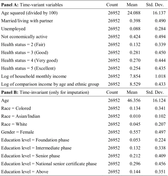
Table 1 shows the summary statistics of the variables used in this study. The full set of the variables is available for 26,952 observations, consisting of household heads. Panel A lists the standard time-variant control variables included in the previous studies (e.g., Baetschmann et
al., 2015; Ferrer-i-Carbonell & Frijters, 2004; Winkelmann & Winkelmann, 1998). According
to the table, 40% of the samples are married. The shares of unemployed and out of labor force add up to 51%. As for health, nearly 80% of the people report good, very good, and excellent perceived health condition. The base category for the health variables comprises those who answered that their health condition was bad. For income variables, the table reports the log of comparison income to take into account for the relative income effects (e.g., Clark & Oswald, 1996; Ferrer-i-Carbonell, 2005; McBride, 2001; Vendrik & Woltjer, 2007),
as well as their household monthly incomes. By following these previous studies, it is calculated as the average among those who are in the same age group (from 5 years younger to 5 years older) and the same race for each survey round.1
Panel B lists the time-invariant variables. The proportion of Colored, Asian/Indian, and
White are 13.4%, 1%, 4.5%, respectively, and the largest share is the base category (i.e., African), which is 81%. This more or less reflects the actual racial distribution in South Africa. As for education level, the base category is no education and its share is 16.3%. The primary education corresponds to the foundation and the intermediate phases, which add up to 18.5%, and secondary education corresponds to the senior and national senior certificate phases, which add up to 50.8%.
2.2. Poverty Line
Although South Africa is regarded as one of the middle-income countries, its Gini index
1 Racial disparity is one of the most serious social problems in South Africa and there are
is very high due to its high poverty incidence, which is an important social issue. The most commonly used measure for income poverty relies on the World Bank’s $1.25 poverty line.2
In addition to this conventional poverty line, this study uses a national poverty line published by South Africa. They published three national poverty lines in 2012: the food poverty line (R305), the lower-bound poverty line (R416), and the upper-bound poverty line (R577) as of
2008 (Statistics South Africa, 2014). The food poverty line is defined based on nutritional requirements. While the lower-bound and upper-bound poverty lines include non-food items,
the difference is whether those who are below the lines need to sacrifice food in order to obtain non-food items. Since the $1.25 poverty line captures acute poverty, this study uses the
upper bound national poverty line as the national poverty line.3 Note that these poverty lines
are adjusted for the price level.
2.3. Multidimensional Poverty Index (MPI)
MPI consists of three dimensions: education, health, and living standard. In order to construct this index, we need to determine the indicators, weight, and cutoffs. Though there are many ways to choose these criteria, this study uses the one proposed by Alkire and Santos (2014) that is a unified criterion for international comparison. In the NIDS dataset, however, one of its indicators (material of floor) is not available in the first round. Thus, following Finn et al. (2013) and Rogan (2016), who analyze MPI using NIDS dataset by modifying Alkire and Santos’ (2014) approach, we adjust the weight for the indicators under the living standard dimension.
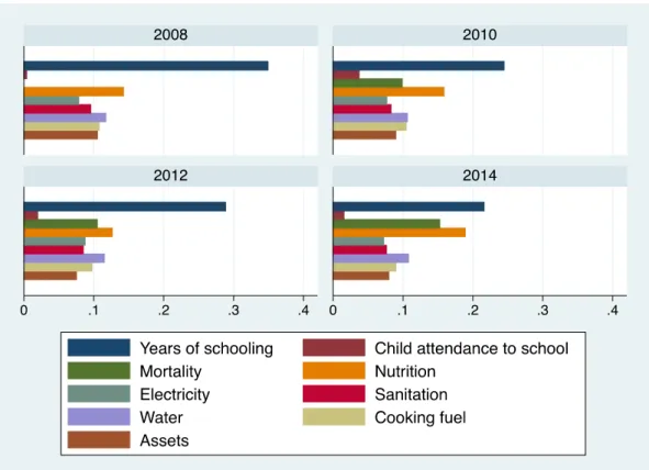
The information used to construct MPI for this study is shown in Table 2. Under the dimensions of education, health, and living standard, there are several indicators with its specific weight. The education dimension is assessed by years of schooling and child attendance to school. The health dimension is assessed by child mortality and nutrition status. The living standard is assessed by whether the household has access to electricity, sanitation, water, cooking fuel, and assets. Note that the weights in each dimension add up to one third, implying that we treat the importance of education, health, and living standard equally.
Using these criteria, the MPI score is calculated for each individual as a weighted sum of the indicators:
2 Note that this poverty line is raised to $1.90 since 2015. However, the data was collected
before 2015. Thus, we use $1.25 as the World Bank’s poverty line.
���� = ∑ ����� �
�=
,
where ��� is a dummy variable, which takes one if the indicator j (= , … , �) is met for individual i and takes zero otherwise. Those who have MPI score lower than the threshold (1/3) are classified as MPI poor. Note that MPI is defined at the household level, and there is no variation among household members. Thus, stacking individual-level observations
violates the iid assumption (Moulton, 1986). In order to avoid this issue, we restrict the sample only to household heads.
An important characteristic of MPI is that it can determine the contributions of each indicator to overall MPI poverty (e.g., Alkire & Santos, 2014). Specifically, we can obtain each indicator’s contribution to MPI by calculating each indicator’s average among those who are identified as MPI poor with its weight. Figure 1 shows the share of each contribution by each survey round. Note that the share of mortality is missing in 2008 because there is no variation due to missing values. Lack of education and mortality account for the largest part of MPI. In contrast, child school attendance has the smallest share, probably reflecting high attendance rate in primary education achieved in recent years. The shares of other indicators are more or less equal, except for the conspicuous high share of nutrition in 2014.
2.4. Distribution of SWB, Income Poverty, and MPI
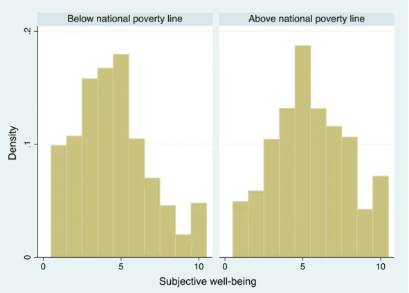
SWB in this dataset is elicited by asking the following question: “Using a scale of 1 to 10 where 1 means “Very dissatisfied” and 10 means “Very satisfied”, how do you feel about your life as a whole right now?” In terms of the national poverty line, 32% of the total population is classified as poor. Figure 2 shows the distribution of SWB by poverty status based on the national poverty line. As is clear from the figure, the distribution is right-skewed
for those below the national poverty line, whereas the distribution is non-skewed for
non-poor. This implies that poor people tend to report lower SWB, while non-poor people do
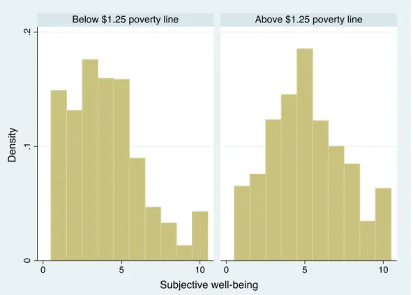
not necessarily report high SWB. This pattern holds even if we use the $1.25 poverty line in Figure 3, where only 3.5% of the people are classified as poor because this poverty line captures more severe poverty. These findings confirm that although there is a positive correlation between SWB and income poverty, these indices are not substitutable.
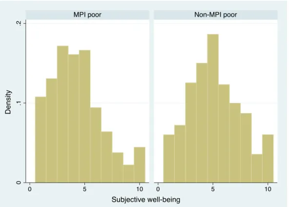
In terms of MPI, 10.3% of the sample is classified as poor. Figure 4 shows the distribution of SWB for those who are MPI poor and non-poor. Similar to income poverty
poor. Thus, the MPI poor also tend to report lower SWB, though the overlap between SWB and MPI is rather limited.
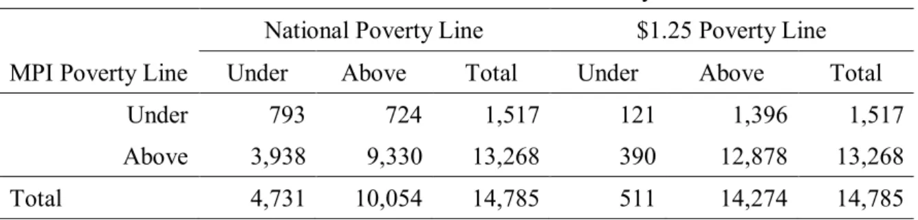
Lastly, Table 3 shows the relationship between income poverty indices and MPI. In this table, diagonal elements overlap between these indices. In terms of the national poverty line, 68.5% of the sample falls in the diagonal element. In terms of the $1.25 poverty line, the share of diagonal elements is 88%. Since MPI is considered to capture severe poverty, these results are reasonable. Pearson’s � test strongly rejects the null hypothesis that income and multidimensional poverty are independent at 1% significance level. However, we also need to note that income poverty and MPI are far from being perfectly substitutable, as 12.1–31.5% of the samples are in off-diagonal elements.
3. Empirical strategy
3.1. Empirical model
This study’s main purpose is to investigate the relationship between SWB, income poverty, and MPI. For this purpose, we estimate the following regression model:
����� = � �(��� < ��) + � � ����� < ���� + ���� + ��+ �� + ���,
(1)
where ����� is i’s SWB at time t, �(��� < ��) and � ����� < ���� are indicator
functions, which take one if their income or MPI score is less than respective poverty lines (�� and ����), ��� is a vector of other controlling variables, �� is survey-round dummies,
�� is individual fixed effects. For the controlling variables, as mentioned above, we follow
the previous studies, which use fixed effect models (Panel A of Table 1). Note that our main parameters of interest are � and � , which represent the effect of objective poverty indices on SWB.
A limitation of specification (1) is that we cannot test the impact of the “intensity” of these indices. For this reason, we also estimate the following model based on Ravallion and Lokshin (2002):
����� = � ln ����
� + � (
�����
���� ) + ���� + ��+ �� + ���.
Note that we do not take log for MPI variable because it lies between 0 and 1, and takes 0 for many observations. Also, note that � is expected to be positive because higher income is associated with higher SWB, while � is expected to be negative because MPI’s higher intensity is associated with lower SWB.
Another advantage of specification (2) is that we can compare the relative importance of income and MPI poverty by discussing how much additional income (relative to poverty line) is necessary to compensate for the decrease in SWB from one-unit change in MPI index (e.g.,
Clark & Oswald, 2002; van Praag et al., 2005; Powdthavee, 2008). Thus, we can address the nexus between income and MPI poverties, which is also an important but a missing issue in the literature.
The problems associated with SWB analysis are: (i) the dependent variable’s ordinal nature, and (ii) the possibility of individual comparison. (i) can be addressed by using ordered response model (e.g., ordered logit/probit model). (ii) can be addressed, albeit partially, by including individual fixed effect to control for the individual-specific mean. However, once
we try incorporating both these issues simultaneously, (e.g., fixed effect ordered logit/probit model), it is difficult to obtain consistent estimates from the standard maximum likelihood (ML) approach because of the incidental parameter problem (e.g., Neyman & Scott, 1948; Lancaster, 2000). Recently, however, Baetschmann et al. (2015) developed the Blow-up and
Cluster (BUC) estimator of fixed effects ordered logit model by extending the conditional ML approach. Specifically, their approach is to maximize the following log-likelihood
function: ��� � ≡ �� (� ��= ��| ∑ ���� = �� � �= ) = ∑ ��� ���� ��′��� �′��� �∈�� ����� � = ∑ ∑ ���{� �� � } � �= � �= ,
where �� and � denote the vectors of dependent variables and their coefficients,
respectively, ��� denotes the binary dependent variable, resulting from dichotomizing the
ordered at the cut-off point k: ��� = (���, … , ����)′ = �� , … , ��� ′ with ��� ∈ { , }, �� =
∑��= ���, and �� = {� ∈ { , }�| ∑��= ��= ��}. Note that it “blows up” the sample size by
finite sample properties. Thus, we estimate fixed effect ordered logit models for specifications (1) and (2) by employing BUC approach.
Another important statistic for this study is the coefficient of determination. Since we are interested in the overlap of the three indices, it is informative to see how much of the variation in SWB can be explained by income poverty and MPI. One straightforward way is to use pseudo-R2 (McFadden, 1974). However, this measure is known to be downward-biased
in our case (Veall & Zimmerman, 1996). By following Ravallion and Lokshin (2002), this study uses (normalized) Aldrich and Nelson pseudo-R2, defined as:
��� =���/ ��� + �− � / � − � ,
where ��� = ��− � , � and �� are the values of log-likelihood with a restriction that
non-intercept coefficients are zero and without any restriction, respectively, and � is the
number of observation. By using this measure, we can discuss the substitutability between SWB and objective poverty indices.
3.2. Multiple imputation
One of the problems of using MPI index is its missing values. Since MPI comprises nine component variables in this study, it cannot be calculated for observations with missing values in at least one of them. Due to this, MPI tends to suffer from missing observations and the resulting sample size becomes smaller. One way to deal with this problem is to ignore the missing values (list-wise deletion), though it can be a source of bias or inefficiency.
In order to deal with this issue, we employ Multivariate Imputation by Chained Equations (MICE) approach. The variables used for the imputation are listed in Table 1. Panel A shows the variables, also included in the main analysis. Panel B shows the time-invariant variables
used only for imputation. Following Graham et al. (2007), we set the number of the simulated data (D) to 40. Using Rubin’s rule (Rubin, 1987), the coefficient estimates and their variance are given by:
�̅� = � ∑ �̂� �
�� = � ∑�� � �= + ( + �)(� − ∑(�̂ �− �̅�) � �= ),
where �̂� and �� are the coefficient estimates and the variance, respectively, from each
imputed dataset d. Note that we calculate Aldrich and Nelson pseudo-R2 as the average of
each dataset.
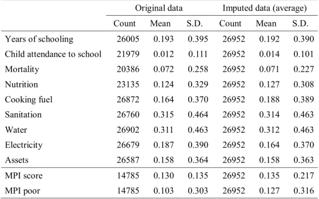
Table 4 shows the summary statistics of the MPI indicators for the original and imputed data. For the imputed data, the averages of the 40 simulated datasets are shown. In the original data, about 45% of the observation is missing in the MPI variables. This results from missing observations especially in child school attendance, mortality, and nutrition indicators. In the imputed dataset, the mean and variance are almost unchanged from the original dataset. The resulting MPI score is slightly higher than the original data, though the number of MPI poor is slightly lower, implying that the share of marginal non-MPI poor people tends to be
missing in the original dataset. In the following analysis, we use these imputed MPI variables.4
4. Results
4.1. SWB and poverty indices
First, we look at the effect of each poverty index on SWB, separately. Table 5 shows the estimation results of the impact of being below income and MPI poverty lines. First three columns show the results using the national poverty line. Being income poor significantly aggravates SWB. However, once we control for household income in column (2), it becomes insignificant while income itself has a significantly positive effect on SWB. Note that this result does not mean income poverty does not affect SWB. Rather, it means that lower income does lead to lower SWB, but that having income lower than the poverty line has no additional effect after controlling for income. Similar pattern can be found when we use $1.25 poverty line in columns (4)–(6).
Column (7) shows that the effect of being MPI poor also significantly aggravates SWB. However, similar to income poverty indices, the significance vanishes after controlling for household income in columns (8) and (9). This also implies that MPI has no additional information to determine SWB compared to household income.
In terms of Aldrich and Nelson pseudo-R2, the objective poverty indices themselves
explain only 6% of the variation in SWB and it increases only to about 7% even after controlling for other independent variables. In other words, 92–93% of the variation remains unexplained. Therefore, the welfare measured by SWB is different from what is measured by objective welfare index.
It is also informative to examine the effect of other control variables. In contrast to the previous studies (e.g., Alesina et al., 2004; Clark & Oswald, 2002; Oswald, 1997), we do not find a significant positive effect of being married. Also, the effect of comparison income is not significant, though the signs are negative. This probably reflects the low social mobility in South Africa, where it is difficult to form aspiration on their income level (Adato et al., 2006; Piraino, 2015). However, we do find some results in line with the previous studies (e.g., Alesina et al., 2004; Baetschmann et al., 2015; Blanchflower & Oswald, 2004; Clark & Oswald, 1994; Deaton & Paxson, 1994; Easterlin, 2001; Ferrer-i-Carbonell & Frijters, 2004;
Frey & Stutzer, 2000; Oswald, 1997; Winkelmann & Winkelmann, 1998): the effect of age is U-shape; being unemployed leads to lower SWB even after controlling for income; better
health condition significantly enhances SWB.
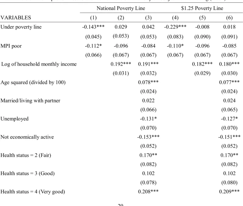
Table 6 shows the estimation results of specification (1), which compares the impact of being below income and MPI poverty lines. Without controlling variables, both being income poor and MPI poor, both significantly aggravate SWB. In this sense, these two metrics capture somewhat different aspects of poverty. However, consistent with Table 5, both effects become insignificant once the effect of income is controlled for. Thus, both measures have no additional information to income. The same pattern holds even if we use $1.25 poverty line in columns (4)–(6).
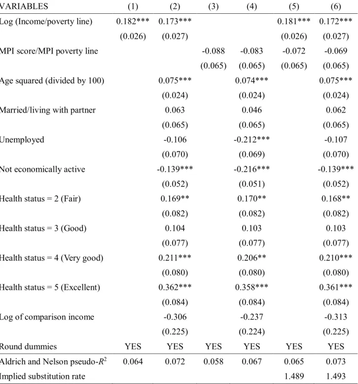
4.2. SWB and intensity of poverty
Table 7 shows the estimation results of specification (2), which analyzes the effect of the intensity of each poverty measure. Since there is no variation in the income poverty line after controlling for the survey round dummies, the choice between the national poverty line and the $1.25 poverty line does not affect the estimation results. For this reason, only the results using the national poverty line are shown in the table.
The effect of income measured by the poverty line is significantly positive, which is consistent with Ravallion and Lokshin (2002). However, MPI’s effect is insignificant, though the coefficient’s sign is negative. Therefore, MPI itself is not a good predictor of SWB, while it may be suitable to identify severe poverty. In terms of Aldrich and Nelson pseudo-R2, a
overlap between subjective and objective welfare measures.5 Other qualitative results remain
virtually unchanged from Tables 5 and 6.
As discussed above, we can calculate the substitution rate between income and multidimensional poverty indices using the coefficient estimates. Although the coefficient is insignificant, the calculated substitution rates are about 1.49 in both columns (5) and (6). This implies that around 1.5 times more poverty line income is necessary to compensate for the decrease in SWB from one unit change in MPI index. In this sense, MPI is a more acute poverty measure than income poverty in terms of SWB.
4.3. Principal component analysis
One fundamental problem with MPI is that its indicators and weights are arbitral (e.g., Ravallion, 2011). As for the weight, the most straightforward way is to include all the indicators separately instead of MPI. However, this approach is inappropriate in our case because some of the indicators are virtually time-invariant and the coefficients estimated
from the fixed effect model are difficult to interpret. In order to create MPI without relying on the pre-determined weight, we employ principal component analysis (PCA)—a standard
approach to create a composite variable (e.g., Alkire et al., 2015; Slottje, 1991).6
Table 8 shows the estimated eigenvectors, which is an average of the results from 40 imputed datasets. Interestingly, the weight on child school attendance, mortality, and nutrition is very small. In contrast, indicators under the living standard dimension have the highest and more or less the same weights except for sanitation. These findings show clear difference from conventional weights.
Using the estimated eigenvector, we can calculate the score as an alternative measure of MPI. However, two important differences should be noted. First, in contrast to the conventional MPI, the weights do not add up to one. This is because PCA maximizes the variance with the constraint that the sum of the squares of the weights is equal to one. Second, before calculating its eigenvectors, we need to normalize the variables by subtracting their means and dividing by their standard deviation. Thus, the mean of the calculated score is also zero. For these reasons, it cannot be treated as the conventional MPI, and therefore we include the calculated score directly instead of �����/���� in the equation (2).
5 R2 is lower than the ones in Ravallion and Lokshin (2002), probably because their
dependent variable is the subjective assessment on economic welfare, not life in general.
6 PCA assumes all component indices are proxies for the same concept; this might be a
The estimated results are shown in Table 9. In contrast to the conventional MPI in Table 7, the MPI score based on PCA has a significantly negative impact, robust to the inclusion of income and other controlling variables. This suggests a complementarity between income poverty and PCI-based MPI in terms of SWB. In this sense, MPI should be constructed based
on PCA, instead of pre-determined weights, in order to fully utilize the data variation. The
magnitude of other controlling variables remains virtually unchanged from Table 7. The implied substitution rate is around 1.2—smaller than the conventional MPI.
5. Concluding remarks
This study investigated the relationship between subjective well-being and objective
poverty indices (i.e., income poverty and MPI). Although these indices are popular in both academics and policymaking, rigorous econometric analysis on their relationship has seldom been conducted. In order to fill this existing gap in the literature, we applied the Blow-up and
Cluster estimation for fixed effect ordered logit model that enabled us to handle the potential problems associated with SWB analysis.
Using a panel data collected in South Africa, we found that both income and multidimensional poverties significantly aggravate SWB. However, the effect of these two metrics becomes insignificant once the effect of household income is controlled for. This implies that the two metrics have no additional information compared to income. However, when we construct MPI based on PCA, the effect of being MPI poor has robust negative effect on SWB, casting a doubt on using pre-determined weight. In terms of the
substitutability between income and multidimensional poverties, we found that being MPI poor is about 1.5 times more severe than income poverty in terms of SWB. Thus, MPI can be regarded as a poverty measure acute than income poverty, intended by Alkire and Santos (2014). Additionally, being below the income poverty lines does not lead to lower SWB if we control income. This implies that the threshold defined by the poverty lines has no additional information on SWB.
Appendix: Estimation using original data
As mentioned, one of the problems of constructing MPI is that it cannot be calculated for a person whose observation is missing in at least one of the indicators. Since the loss of the observations due to this reason is not negligible in this dataset, we imputed the data by employing the multiple imputation method. However, it is also informative to see how estimation results change without using this approach. For this reason, we estimate the model using the original dataset (i.e., without imputed values).
Estimation results are shown in Tables A1 and A2. Comparing to the corresponding results using multiple imputation in Tables 5, 6, and 7, the effect of being MPI poor has a significantly negative impact on SWB, and the effect is robust to the inclusion of controlling variables. This contrast comes from non-random missing observations in the variables
References
Adato, M., M. R. Carter, & J. May. (2006). Exploring poverty traps and social exclusion in South Africa using qualitative and quantitative data. Journal of Development Studies, 42(2), 226–247.
Alesina, A., R. Di Tella, & R. MacCulloch. (2004). Inequality and Happiness: Are Europeans and Americans different? Journal of Public Economics, 88(9–10), 2009–42.
Alkire, S. & J. Foster. (2011). Understandings and misunderstandings of multidimensional poverty measurement. Journal of Economic Inequality,9(2), 289–314.
Alkire, S. & J. Foster. (2011). Counting and multidimensional poverty measurement. Journal of Public Economics,95, 476–487.
Alkire, S., J. Foster, S. Seth, M. E. Santos, J. M. Roche, & P. Ballon. (2015).
Multidimensional Poverty Measurement and Analysis. Location: Oxford University Press.
Alkire, S. & M. E. Santos. (2014). Measuring Acute Poverty in the Developing World: Robustness and Scope of the Multidimensional Poverty Index. World Development, 59, 251–274.
Baetschmann, G., K. E. Staub & R. Winkelmann. (2015). Consistent estimation of the fixed effects ordered logit model. Journal of the Royal Statistical Society, Statistics in Society, Series A, 178(3), 685–703.
Banerjee, A. & E. Duflo. (2011). Poor Economics: A Radical Rethinking of the Way to Fight Global Poverty. New York: PublicAffairs.
Blanchflower, D. G. & A. J. Oswald. (2004). Well-being over time in Britain and the USA.
Journal of Public Economics, 88(7–8), 1359–86.
Bourguignon, F. & S. R. Chakravarty. (2003). The Measurement of Multidimensional Poverty.
Journal of Economic Inequality,1(1), 25–49.
Chakravarty, S. R., J. Deutsch, & J. Silber. (2008). On the Watts Multidimensional Poverty Index and its Decomposition. World Development,36(6), 1067–77.
Clark, A. E. & A. J. Oswald. (1996). Satisfaction and comparison income. Journal of Public Economics,61(3), 359–381.
Clark, A. E. & A. J. Oswald. (2002). A simple statistical method for measuring how life events affect happiness. International Journal of Epidemiology,31(6), 1139–1144.
Comparison of Various Approaches. Review of Income and Wealth,51(1), 145–74.
Duclos, J-Y, D. E. Sahn, & S. D. Younger. (2006). Robust Multidimensional Poverty
Comparisons. Economic Journal,116(514), 943–68.
Easterlin, R. A. (2001). Income and happiness: Towards a unified theory. Economic Journal, 111(473), 465–84.
Ferrer-i-Carbonell, A. (2005). Income and well-being: An empirical analysis of the
comparison income effect. Journal of Public Economics, 89(5–6), 997–1019.
Ferrer-i-Carbonell, A. & P. Frijters. (2004). How Important Is Methodology for The
Estimates of The Determinants of Happiness? Economic Journal,114(497), 641–659. Finn, A. & M. Leibbrandt. (2013). The Dynamics of Poverty in the First Three Waves of
NIDS. (NIDS Discussion Paper No. 119). Location: Publisher.
Finn, A., Leibbrandt, M., & Woolard, I. (2013). What happened to multidimensional poverty in South Africa between 1993 and 2010? (Southern Africa Labour and Development Research Unit Working Paper No. 99). Location: Publisher.
Ferreira, F. H. G. & M. A. Lugo. (2013). Multidimensional Poverty Analysis: Looking for a Middle Ground. World Bank Research Observer, 28(2), 220–235.
Frey, B. S. & A. Stutzer. (2002). What Can Economists Learn from Happiness Research?
Journal of Economic Literature, 40(2), 402–435.
Gradin, C. (2012). Race, Poverty and Deprivation in South Africa. Journal of African Economies, 22(2), 187–238.
Graham, J. W., A. E. Olchowski, & T. D. Gilreath. (2007). How Many Imputations are Really Needed? Some Practical Clarifications of Multiple Imputation Theory. Prevention Science,8(3), 206–213.
Helliwell, J., R. Layard & J. Sachs. (2016). World Happiness Report 2016. Retrieved from http://worldhappiness.report/wp-content/uploads/sites/2/2016/03/HR-V1_web.pdf
Kingdon, G. G. & J. Knight. (2006). Subjective well-being poverty vs. Income poverty and
capabilities poverty? Journal of Development Studies, 42(7), 1199–1224.
Lancaster, T. (2000). The incidental parameter problem since 1948. Journal of Econometrics,
95(2), 391–413.
McBride, M. (2001). Relative-income effects on subjective well-being in the cross-section.
Journal of Economic Behavior & Organization, 45(3), 251–278.
Moulton, B. R. (1986). Random Group Effects and the Precision of Regression Estimates.
Journal of Econometrics,32(3), 385–97.
Neff, D. F. (2007). Subjective Well-Being, Poverty and Ethnicity in South Africa: Insights
Neyman, J. & E. L. Scott. (1948). Consistent Estimates Based on Partially Consistent Observations. Econometrica, 16(1), 1–32.
OECD. (2013). OECD Guidelines on Measuring Subjective Well-being. Location: OECD
Publishing.
Oswald, A. J. (1997). Happiness and economic performance. Economic Journal, 107(445), 1815–31.
Piraino, P. (2015). Intergenerational Earnings Mobility and Equality of Opportunity in South Africa. World Development, 67, 396–405.
Powdthavee, N. (2007). Happiness and the Standard of Living: The Case of South Africa. In Bruni, L. & Porta, P.L. (Eds.), Handbook on the Economics of Happiness (447–486). Edward Elgar: UK.
Powdthavee, N. (2008). Putting a price tag on friends, relatives, and neighbours: Using surveys of life satisfaction to value social relationships. Journal of Socio-Economics,
37(4), 1459–1480.
Ravallion, M. (2011). Mashup Indices of Development. World Bank Research Observer, 27(1), 1–32.
Ravallion, M. (2011). On multidimensional indices of poverty. Journal of Economic Inequality,9(2), 235–248.
Ravallion, M. (2016). The Economics of Poverty: History, Measurement, and Policy. Location: Oxford University Press.
Ravallion, M. & M. Lokshin. (2002). Self-rated economic welfare in Russia. European
Economic Review,46(8), 1453–1473.
Rogan, M. (2016). Gender and Multidimensional Poverty in South Africa: Applying the Global Multidimensional Poverty Index (MPI). Social Indicators Research, 126(3), 987–1006.
Rojas, M. (2008). Experienced Poverty and Income Poverty in Mexico: A Subjective Well-Being Approach. World Development, 36(6), 1078–1093.
Rubin, D. (1987). Multiple Imputation for Nonresponse in Surveys. New York: John Wiley. Sen, A. (1985). Commodities and Capabilities. Amsterdam, New York, North-Holland:
Elsevier.
Slottje, D. J. (1991). Measuring the Quality of Life Across Countries. Review of Economics and Statistics,73(4), 684–93.
df
Stiglitz, J. E., A. Sen, & J. Fitoussi. (2009). Report by the Commission on the Measurement of Economic Performance and Social Progress. Location: Commission on the Measurement of Economic Performance and Social Progress, Paris.
Tsui, K-Y. (2002). Multidimensional Poverty Indices. Social Choice and Welfare, 19(1), 69–
93.
van Praag, B. M. S. & B. E. Baarsma. (2005). Using Happiness Surveys to Value Intangibles: The Case of Airport Noise. Economic Journal, 115(500), 224–246.
Veall, M. R. & K. F. Zimmermann. (1996). Pseudo-R2 measures for some common limited
dependent variable models. Journal of Economic Surveys,10(3), 241–259.
Vendrik, M. C.M. & G. B. Woltjer. (2007). Happiness and loss aversion: Is utility concave or convex in relative income? Journal of Public Economics,91(7–8),1423–1448.
Table 1: Descriptive Statistics of Sample Individuals
Panel A: Time-variant variables Count Mean Std. Dev.
Age squared (divided by 100) 26952 24.088 16.137
Married/living with partner 26952 0.398 0.490
Unemployed 26952 0.088 0.284
Not economically active 26952 0.424 0.494
Health status = 2 (Fair) 26952 0.132 0.339
Health status = 3 (Good) 26952 0.281 0.450
Health status = 4 (Very good) 26952 0.270 0.444
Health status = 5 (Excellent) 26952 0.254 0.435
Log of household monthly income 26952 7.854 1.018
Log of comparison income by age and ethnic group 26952 8.529 0.433
Panel B: Time-invariant (only for imputation) Count Mean Std. Dev.
Age 26952 46.356 16.124
Race = Colored 26952 0.134 0.341
Race = Asian/Indian 26952 0.010 0.102
Race = White 26952 0.045 0.207
Gender = Female 26952 0.557 0.497
Education level = Foundation phase 26952 0.053 0.224
Education level = Intermediate phase 26952 0.132 0.338
Education level = Senior phase 26952 0.212 0.409
Education level = National senior certificate phase 26952 0.296 0.456
Table 2: Indicators and Weights for the Multidimensional Poverty Index
Indicator Weight Deprived if…
Education:
Years of schooling 1/6 No household member has completed 5 years of schooling
Child attendance to school 1/6 Any school-aged child is not attending primary school
Health:
Mortality 1/6 Any child has died in the family in the last 20 years
Nutrition 1/6
Any adult whose BMI is below 18.5 or children whose
z-score of weight-for-age is below minus two standard
deviations from the median of the reference population
Living standard:
Electricity 1/15 The household has no electricity.
Sanitation 1/15 The household has no flush toilet or latrine, or ventilated
improved pit or chemical toilet; provided that it is not
shared.
Water 1/15 The household does not have access to piped water or
public tap.
Cooking fuel 1/15 The household cooks with dung, wood, or carbon.
Assets 1/15 The household does not own one of the following assets:
radio, TV, telephone, bicycle, motorbike, refrigerator, and
does not own a car or truck.
Table 3: Income and Multidimensional Poverty Indices
National Poverty Line $1.25 Poverty Line
MPI Poverty Line Under Above Total Under Above Total
Under 793 724 1,517 121 1,396 1,517
Above 3,938 9,330 13,268 390 12,878 13,268
Table 4: Summary Statistics for Multidimensional Poverty Indicators (Original and Imputed Data)
Original data Imputed data (average)
Count Mean S.D. Count Mean S.D.
Years of schooling 26005 0.193 0.395 26952 0.192 0.390
Child attendance to school 21979 0.012 0.111 26952 0.014 0.101
Mortality 20386 0.072 0.258 26952 0.071 0.227
Nutrition 23135 0.124 0.329 26952 0.127 0.308
Cooking fuel 26872 0.164 0.370 26952 0.188 0.389
Sanitation 26760 0.315 0.464 26952 0.314 0.463
Water 26902 0.311 0.463 26952 0.312 0.463
Electricity 26679 0.187 0.390 26952 0.164 0.370
Assets 26587 0.158 0.364 26952 0.158 0.363
MPI score 14785 0.130 0.135 26952 0.135 0.217
Table 5: The Impact of Income and Multidimensional Poverty on Subjective Well-being (Index)
National Poverty Line $1.25 Poverty Line Multidimensional Poverty
VARIABLES (1) (2) (3) (4) (5) (6) (7) (8) (9)
Below poverty line -0.144*** 0.030 0.043 -0.233*** -0.009 0.017
(0.045) (0.053) (0.053) (0.083) (0.090) (0.091)
MPI poor -0.114* -0.096 -0.085
(0.066) (0.067) (0.067)
Log of household monthly income 0.194*** 0.192*** 0.184*** 0.182*** 0.183*** 0.178***
(0.031) (0.032) (0.029) (0.030) (0.027) (0.027)
Age squared (divided by 100) 0.079*** 0.078*** 0.077***
(0.024) (0.024) (0.024)
Married/living with partner 0.021 0.023 0.024
(0.066) (0.066) (0.065)
Unemployed -0.131* -0.127* -0.126*
(0.070) (0.070) (0.070)
Not economically active -0.153*** -0.151*** -0.150***
(0.052) (0.052) (0.052)
Health status = 2 (Fair) 0.170** 0.171** 0.170**
(0.082) (0.082) (0.082)
Health status = 3 (Good) 0.103 0.104 0.102
(0.080) (0.080) (0.080)
Health status = 5 (Excellent) 0.362*** 0.364*** 0.362***
(0.084) (0.084) (0.084)
Log of comparison income -0.317 -0.315 -0.319
(0.225) (0.225) (0.225)
Round dummies YES YES YES YES YES YES YES YES YES
Aldrich and Nelson pseudo-R2 0.059 0.064 0.072 0.059 0.064 0.072 0.058 0.064 0.073
Table 6: The Impact of Income and Multidimensional Poverty on Subjective Well-being (Index)
National Poverty Line $1.25 Poverty Line
VARIABLES (1) (2) (3) (4) (5) (6)
Under poverty line -0.143*** 0.029 0.042 -0.229*** -0.008 0.018
(0.045) (0.053) (0.053) (0.083) (0.090) (0.091)
MPI poor -0.112* -0.096 -0.084 -0.110* -0.096 -0.085
(0.066) (0.067) (0.067) (0.067) (0.067) (0.067)
Log of household monthly income 0.192*** 0.191*** 0.182*** 0.180***
(0.031) (0.032) (0.029) (0.030)
Age squared (divided by 100) 0.078*** 0.077***
(0.024) (0.024)
Married/living with partner 0.022 0.024
(0.066) (0.065)
Unemployed -0.131* -0.127*
(0.070) (0.070)
Not economically active -0.153*** -0.151***
(0.052) (0.052)
Health status = 2 (Fair) 0.170** 0.170**
(0.082) (0.082)
Health status = 3 (Good) 0.102 0.102
(0.080) (0.080) Health status = 5 (Excellent) 0.361*** 0.362***
(0.084) (0.084)
Log of comparison income -0.320 -0.319
(0.225) (0.225)
Round dummies YES YES YES YES YES YES
Aldrich and Nelson pseudo-R2 0.059 0.064 0.073 0.059 0.064 0.073
Table 7: The Impact of Income and Multidimensional Poverty on Subjective Well-being (Intensity)
VARIABLES (1) (2) (3) (4) (5) (6)
Log (Income/poverty line) 0.182*** 0.173*** 0.181*** 0.172***
(0.026) (0.027) (0.026) (0.027)
MPI score/MPI poverty line -0.088 -0.083 -0.072 -0.069
(0.065) (0.065) (0.065) (0.065)
Age squared (divided by 100) 0.075*** 0.074*** 0.075***
(0.024) (0.024) (0.024)
Married/living with partner 0.063 0.046 0.062
(0.065) (0.065) (0.065)
Unemployed -0.106 -0.212*** -0.107
(0.070) (0.069) (0.070)
Not economically active -0.139*** -0.216*** -0.139***
(0.052) (0.051) (0.052) Health status = 2 (Fair) 0.169** 0.170** 0.168**
(0.082) (0.082) (0.082) Health status = 3 (Good) 0.104 0.103 0.103
(0.077) (0.077) (0.077) Health status = 4 (Very good) 0.211*** 0.206** 0.210***
(0.080) (0.080) (0.080) Health status = 5 (Excellent) 0.362*** 0.358*** 0.361***
(0.084) (0.084) (0.084)
Log of comparison income -0.306 -0.237 -0.313
(0.225) (0.224) (0.225)
Round dummies YES YES YES YES YES YES
Aldrich and Nelson pseudo-R2 0.064 0.072 0.058 0.067 0.065 0.073
Implied substitution rate 1.489 1.493
Table 8: Principal Component (Eigenvectors)
Component
(Average)
Education:
Years of schooling 0.298
Child attendance to school 0.058
Health:
Mortality 0.061
Nutrition 0.055
Living standard:
Cooking fuel 0.505
Sanitation 0.175
Water 0.453
Electricity 0.468
Table 9: The Impact of Income and Multidimensional Poverty on Subjective Well-being Using Principal Component Analysis
VARIABLES (1) (2) (3)
Log (Income/poverty line) 0.180*** 0.171***
(0.026) (0.027)
MPI score (principal component) -0.041** -0.034* -0.036*
(0.020) (0.020) (0.020)
Age squared (divided by 100) 0.075***
(0.024)
Married/living with partner 0.061
(0.065)
Unemployed -0.108
(0.070)
Not economically active -0.138***
(0.052) Health status = 2 (Fair) 0.169**
(0.082) Health status = 3 (Good) 0.104
(0.077) Health status = 4 (Very good) 0.212***
(0.080) Health status = 5 (Excellent) 0.363***
(0.084)
Log of comparison income -0.328
(0.225)
Round dummies YES YES YES
Aldrich and Nelson pseudo-R2 0.058 0.065 0.073
Implied substitution rate 1.208 1.234
Table A1: The Impact of Income and Multidimensional Poverty on Subjective Well-being (Index): Original Data
Multidimensional Poverty National Poverty Line $1.25 Poverty Line
VARIABLES (1) (2) (3) (4) (5) (6) (7) (8) (9)
Below poverty line -0.140* 0.048 0.051 -0.149 0.105 0.123
(0.079) (0.093) (0.093) (0.166) (0.177) (0.179)
MPI poor -0.295** -0.279** -0.272** -0.287** -0.280** -0.273** -0.291** -0.280** -0.273**
(0.121) (0.122) (0.121) (0.122) (0.122) (0.122) (0.121) (0.122) (0.121)
Log of household monthly income 0.170*** 0.163*** 0.185*** 0.178*** 0.180*** 0.174***
(0.043) (0.044) (0.050) (0.051) (0.045) (0.047)
Age squared (divided by 100) 0.065* 0.066* 0.066*
(0.039) (0.039) (0.039)
Married/living with partner 0.031 0.029 0.032
(0.104) (0.104) (0.104)
Unemployed -0.133 -0.139 -0.136
(0.107) (0.108) (0.107)
Not economically active -0.072 -0.077 -0.076
(0.087) (0.087) (0.087)
Health status = 2 (Fair) 0.071 0.069 0.072
(0.170) (0.170) (0.170)
Health status = 3 (Good) 0.122 0.120 0.122
(0.158) (0.158) (0.158)
(0.162) (0.162) (0.161)
Health status = 5 (Excellent) 0.392** 0.389** 0.393**
(0.165) (0.165) (0.164)
Log of comparison income 0.605 0.607 0.606
(0.425) (0.424) (0.424)
Round dummies YES YES YES YES YES YES YES YES YES
Table A2: The Impact of Income and Multidimensional Poverty on Subjective Well-being (Intensity)
VARIABLES (1) (2) (3)
Log (Income/poverty line) 0.177*** 0.174***
(0.042) (0.044)
MPI score/MPI poverty line -0.234** -0.197* -0.188
(0.119) (0.119) (0.120)
Age squared (divided by 100) 0.066*
(0.039)
Married/living with partner 0.069
(0.104)
Unemployed -0.107
(0.109)
Not economically active -0.045
(0.088) Health status = 2 (Fair) 0.087
(0.171) Health status = 3 (Good) 0.136
(0.159) Health status = 4 (Very good) 0.286* (0.162) Health status = 5 (Excellent) 0.404**
(0.165)
Log of comparison income 0.572
(0.426)
Round dummies YES YES YES
Aldrich and Nelson pseudo-R2 0.050 0.057 0.065
Implied substitution rate 3.043 2.946