R ESEARCH I NSTITUTEFOR M ATHEMATICAL S CIENCESKYOTOUNIVERSITY,Kyoto,Japan ByHiroshiHIRAIOctober2008 K + K andrelatedmaximizationproblems Boundedfractionalityofthemultiflowfeasibilityproblemfordemandgraph RIMS-1645

RIMS-1645

Bounded fractionality of the multiflow feasibility problem for demand graph K

+ K

and related

maximization problems

By

Hiroshi HIRAI

October 2008

R ESEARCH I NSTITUTE FOR M ATHEMATICAL S CIENCES

KYOTO UNIVERSITY, Kyoto, Japan

Bounded fractionality of the multiflow feasibility problem for demand graph K ₃ + K ₃ and related

maximization problems

Hiroshi HIRAI

Research Institute for Mathematical Sciences, Kyoto University, Kyoto 606-8502, Japan

[email protected]

October 2008

Abstract

We consider the multiflow feasibility problem whose demand graph is the vertex-disjoint union of two triangles. We show that this problem has a 1/12-integral solution or no solution under the Euler condition. This solves a conjecture raised by Karzanov, and completes the classification of the demand graphs having bounded fractionality. We reduce this problem to the multiflow maximization problem whose terminal weight is the graph metric of the complete bipartite graphKn,m, and show that it always has a 1/12-integral optimal multiflow for every inner Eulerian graph.

1 Introduction

Let G = (V G, EG) be an undirected graph with nonnegative edge capacity c : EG → R₊, and let S ⊆ V G be a set of terminals. Let H = (S, R) be another (simple) graph on S, which is called a demand graph. A (simple) path P in G is called anS-path if its ends belong to distinct nodes of S. A multiflow f = (P, λ) is a pair of a setP ofS-paths and its nonnegative flow-value functionλ:P →R₊ satisfying the capacity constraint

∑{λ(P)|P ∈ P :P contains e} ≤c(e) (e∈EG).

For a demand functionq :R→R₊, themultiflow feasibility problem with respect to (G, c;H, q) is:

(1.1) Find a multiflowf satisfying the demand requirement

∑{λ(P)|P ∈ P :P is an (s, t)-path}=q(st) (st∈R),

or establish that there is no such a multiflow.

The classical max-flow min-cut theorem, due to Ford-Fulkerson [2], says that ifHis one edgeK₂ (or a star),candqare integral and if a feasible solution exists, then an integral feasible solution also exists. Hu [6] extended this result to two-commodity flows, saying that ifH =K₂+K₂ (a matching of size 2),candqare integral and if a feasible solution exists, then a half-integral feasible solution also exists. On the other hand, the 3-commodity flow problem, that corresponds toH =K2+K2+K2

(a matching of size 3), does not have such a property. Lomonosov [14] gave an infinite series of the feasible integer-capacitated 3-commodity flow problems with integer demands in which there is no fixed integer k such that all these problems have a 1/k-integral feasible solution; see [17, Chapter 70, p.1232].

Motivated by these examples, following [9], we define the fractionality of a (simple) demand graphHby the least positive integerk with the property that for every integer-capacitated graph having H as a demand graph with every integral demand a 1/k-integral feasible solution exists whenever a feasible solution exists.

If such a integer k never exists, we define the fractionality to be the infinity.

Karzanov raised the problem:

(1.2) Characterize the demand graph H having bounded fractionality.

Lomonosov’s 3-commodity example above implies that ifH has a matching of size 3, then the fractionality ofH is infinity. Therefore, for the problem (1.2), we may restrict to consider the demand graphs without a matching of size 3. Such a graph (except a star) falls into one of the following three classes:

(i) K₄,C₅, or the union of two stars.

(ii) K₅ or the union of a star and a triangleK₃.

(iii) K3+K3, i.e., the vertex-disjoint sum of two triangles.

For the class (i), the works by Rothschild and Winston [15], Seymour [18] and Lomonosov [14] imply the following. Here, we say “(G, c;H, q) satisfies the Euler condition” if the graph G+H = (V G, EG∪R) with capacity c+q is Eulerian.

Theorem 1.1([15, 18, 14]). Suppose that H is K₄, C₅, or the union of two stars, and(G, c;H, q) satisfies the Euler condition. If a feasible multiflow exists, then an integral feasible multiflow exists.

In particular, the graphs of the class (i) have fractionality 2. Karzanov [8]

showed that the same result holds for the graphs of the class (ii).

Theorem 1.2 ([8]). Suppose that H is K₅ or the union of a star and a triangle, and(G, c;H, q) satisfies the Euler condition. If a feasible multiflow exists, then an integral feasible multiflow exists.

For the remaining last class (iii): H =K₃+K₃, it is known that the fractionality is greater than or equal to 4; see [17, p. 1275]. Karzanov [10] conjectured that K₃+K₃ has bounded fractionality, and also conjectured, more strongly, that under the Euler condition the existence of a feasible multiflow implies the existence of a half-integral feasible multiflow, and in particular the fractionality ofH =K₃+K₃

equals the lower bound 4. These two conjectures are also raised as Problem 52 and Problem 51 in Schrijver’s book [17]; also see p. 1274. The main result of this paper solves the weaker conjecture (Problem 52) affirmatively as follows.

Theorem 1.3. Suppose that H is K₃ +K₃, and (G, c;H, q) satisfies the Euler condition. If a feasible multiflow exists, then a 1/12-integral feasible multiflow exists.

This result completes the classification of the demand graphs having bounded fractionality. In particular, the fractionality of H =K₃+K₃ is one of 4,8,12,24.

We however do not know whether the constant 1/12 is tight.

Kn,m-metric-weighted maximum multiflow problem. In fact, the multiflow feasibility problem for H = K₃ +K₃ reduces to a certain multiflow maximiza- tion problem. Let G be an undirected graph with nonnegative edge capacity c and terminals S ⊆ V G. Let Kn,m be the complete bipartite graph having S as vertices. Consider the following multiflow maximization problem (K_n,m-metric- weighted maximum multiflow problem):

Maximize ∑

P∈P

dist_Kn,m(s_P, t_P)λ(P) (1.3)

subject to f = (P, λ): multiflow for (G, c;S),

wheres_P andt_P are the ends ofP, and dist_Kn,m denotes the graph metric induced by K_n,m. Suppose that the bipartition of K_n,m is {A, B}. If a path P ∈ P is an A-path or a B-path, then P contributes 2λ(P) for the objective value of (1.3). If P connects A andB, then P contributes λ(P). (G, c) is said to be inner Eulerian (with respect toS) ifcis integral and every node except the terminals S has even degree. For the case of min(n, m) = 2, Karzanov and Mannoussakis [13] showed that (1.3) has an integral optimal multiflow for every inner Eulerian graph having S as terminals. For the case of min(n, m)≥3, however, such an integrality result does not hold. For example, S is a six-set havingK_3,3, Gis a star havingS as the leafs, and all six edgesEG have unit capacity. Then (1.3) has no integral optimal multiflow (although a half-integral optimal multiflow exists). We will derive the main theorem (Theorem 1.3) from:

Theorem 1.4. Kn,m-metric-weighted maximum multiflow problem (1.3) has a 1/12-integral optimal multiflow for every inner Eulerian graph.

For µ-weighted maximum multiflow problems for a general terminal weight µ : S ×S → R₊, we can define the fractionality of µ in a similar way. Hence dist_Kn,m has bounded fractionality. This result is a step toward the classification of the terminal weights having bounded fractionality. We will further investigate this subject in the next paper [5].

This paper is organized as follows. In Section 2, we describe a combinatorial duality theorem (Theorem 2.1) for (1.3) due to Karzanov [12], and its two op- timality criterions: the first one (Lemma 2.2) is well-known and the second one (Proposition 2.3) is new. We explain a reduction of the feasibility problem for H =K₃ +K₃ to the maximization problem for K_3,3 in Section 2.5. The proof of

the combinatorial duality theorem together with the second optimality criterion is given in Section 2.7. Our proof of Theorem 1.4 is based on a fractional varia- tion of the splitting-off method together with optimality criterions. Section 3 is devoted to the proof. A basic idea and an overview of the proof are described at Section 3.1. Section 4 gives some concluding remarks.

Notation. R and R₊ denote the sets of reals and nonnegative reals, respec- tively. Similarly, Z and Z₊ denote the sets of integers and nonnegative integers, respectively. The set of functions from a setV toR (resp. R₊) is denoted by R^V (resp. R^V₊). For a subsetS of V, the characteristic vectorχ_S ∈R^V is defined by:

χ_S(x) = 1 ifx∈S andχ_S(x) = 0 otherwise. As usual, χ_{s} is denoted byχ_s for a singleton set{s}.

In this paper, by a graph we mean an undirected graph with possible parallel edges and loops. For a graphG, the set of vertices is denoted by V G, and the set of edges is denoted by EG. For an edge e and vertices x, y, the notation e = xy means that e connects x and y. If e is a unique edge connecting vertices x and y, then e is also denoted by xy. We will treat two types of graphs: one is a supply graph G in which multiflows flow, and the other one is a simple graph Γ that represents dual variables (potentials) as its vertices. To distinguish the roles of G and Γ, a vertex of a supply graph G is particularly called a node. A node that is not a terminal is called an inner node.

A path P in G is an alternating sequence (x₁, e₁, x₂, e₂, x₃, . . . , x_m) of nodes and edges with e_i = x_ix_i+1. Without noted, a path P means a simple path, i.e., there are no repeated nodes and edges in P. For two nodes x_i and x_j (i < j) in P, the subpath of P between x_i and x_j is denoted by P(x_i, x_j). For two paths P

=(x₁, e₁, . . . , e_m−1, x_m) andQ= (x_m, e_m, . . . , e_n−1, x_n) having exactly one common end x_m, the concatenation (x₁, e₁. . . , x_m, e_m, . . . , x_n) of P and Q is denoted by P ·Q. When P ·Q is nonsimple, we redefine P · Q by its simplification. For subsetsA₁, A₂, . . . A_m of nodes, a pathP passing A₁, A₂, . . . , A_m in order is called an (A₁, A₂, . . . , A_m)-path. As usual, if A_j is a singleton set {a_j}, we simply say that P is an (A₁, A₂, . . . , a_j, . . . , A_m)-path. In this paper, the terminal set S is partitioned into two sets A and B. For a ∈ A and b ∈ B, A\a and B \b are simply denoted by ¯aand ¯b, respectively. Clearly an A-pathP is an (a,a)-path for¯ some a ∈ A. For a path P and a function d on edges set EG, d(P) denotes the sum of d(e) over edges e in P.

For a multiflow f = (P, λ), P is allowed to be a multiset. Without noted, λ is supposed to be positive, i.e., λ(P) > 0 for every P ∈ P. When λ(P) = 0 occurs in some multiflow manipulation, we always delete P from P. For an edge e, the subset of paths in P passing e is denoted by P(e), and the total sum of its flow-values is denoted byf^e, i.e., f^e=∑

P∈P(e)λ(P).Similarly, for two edges e, e⁰, the subset of paths inP passing bothe ande⁰ is denoted by P(e, e⁰), and the total sum of its flow-values is denoted by f^e,e0.

By a metric d on a set S we mean a function defined on S ×S satisfying d(s, t) = d(t, s)≥d(t, t) = 0 and the triangle inequalities d(s, t) +d(t, u)≥d(s, u) for s, t, u ∈S. We often regard a metric d on V G of a graph G as d :EG →R+

by d(e) = d(x, y) for e = xy. For a graph Γ, the shortest path metric on V Γ by Γ (with unit length) is denoted by dist_Γ.

2 K

-metric-weighted

maximum multiflow problem

Let G be a graph with terminals S ⊆ V G. Suppose that the terminal set S is partitioned into two setsAandB with min{#A,#B} ≥3. Letµ_A,B be the metric onS defined by

(2.1) µ_A,B(s, t) =





4 if s6=t, s, t∈A ors, t ∈B, 2 if (s, t)∈A×B or (t, s)∈A×B, 0 if s=t.

Namelyµ_A,B is twice the graph metric of the complete bipartite graph with bipar- tition {A, B}. For a technical reason, instead of (1.3) we consider the following scaled version:

Maximize ∑

P∈P

µ_A,B(s_P, t_P)λ(P) (2.2)

subject to f = (P, λ) is a multiflow for (G, c;S),

wheres_P and t_P are ends of P. The optimal value of (2.2) is denoted by ν(G, c).

2.1 A combinatorial duality theorem

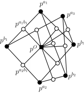
First we describe a combinatorial duality theorem for (2.2), which was (implicitly) described by Karzanov [12]. LetΓ be a simple graph whose vertices V Γ are

p^O, p^a, p^b, p^ab ((a, b)∈A×B), and edges EΓ are

p^Op^ab, p^ap^ab, p^bp^ab ((a, b)∈A×B).

Namely,Γ is the graph obtained by subdividing the complete bipartite graph with bipartition {{p^a}a∈A,{p^b}b∈B} and joining a new point p^O and each subdivided point p^ab. See Figure 1. Note that Γ has µA,B as a submetric, i.e.,

(2.3) µ_A,B(s, t) = dist_Γ(p^s, p^t) (s, t ∈S).

Consider the following discrete location problem (the minimum 0-extension prob- lem) on Γ:

Minimize ∑

e=xy∈EG

c(e)dist_Γ(ρ(x), ρ(y)) (2.4)

subject to ρ:V G→V Γ,

ρ(s) = p^s (s∈S =A∪B).

Theorem 2.1 ([12]). The maximum value of(2.2) is equal to the minimum value of (2.4).

Note that the weak duality is easily seen from (2.3). We call a feasible solution ρ of (2.4) apotential.

p

p

p

p

p

p

p

p

p

Figure 1: GraphΓ forA ={a₁, a₂, a₃}, B ={b₁, b₂, b₃}

2.2 Optimality criterion I

Second we describe the optimality criterion of primal-dual type, which involves both multiflow and potential. For a potential ρ, a metric d^ρ onV G is defined by

d^ρ(x, y) = distΓ(ρ(x), ρ(y)) (x, y ∈V G).

For a multiflow f = (P, λ) and a potential ρ, the objective values of (2.2) and (2.4) are denoted byµ_A,B◦f andhc, d^ρi=hc, d^ρiG, respectively. The weak duality states

µ_A,B◦f ≤ hc, d^ρi. The duality gap hc, d^ρi −µA,B◦f is given by

(2.5) ∑

e∈EG

d^ρ(e)(c(e)−f^e) + ∑

P∈P

λ(P)(d^ρ(P)−µ_A,B(s_P, t_P)).

Therefore the optimality criterion is given as:

Lemma 2.2. A multiflow f = (P, λ) and a potential ρ are optimal to (2.2) and (2.4), respectively, if and only if

∀e=xy∈EG:d^ρ(x, y)>0 ⇒ f^e =c(e), (2.6)

∀P ∈ P :λ(P)>0 ⇒ d^ρ(P) =µ_A,B(s_P, t_P).

Letf = (P, λ) andρbe an optimal multiflow and an optimal potential, respec- tively. Let x be an inner node and P an (s, x, t)-path in P passing x. By (2.6), the ends s and t of P must satisfy

d^ρ(s, x) +d^ρ(x, t) = d^ρ(s, t) = dist_Γ(p^s, p^t).

From this formula, we can determine the ends s, t of P. For example, we have:

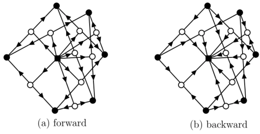
(a) forward (b) backward

Figure 2: (a) forward orientation and (b) backward orientation (2.7) Ifρ(x) =p^O, then P is an A-path or aB-path.

Ifρ(x) =p^a, then P is an (a, B)-path, an (a,¯a)-path, or a B-path.

Ifρ(x) =p^ab, thenP is an (a, b)-path, an (a,¯a)-path, or a (b,¯b)-path.

Lete=xybe an edge withρ(x)6=ρ(y) andP an (s, x, y, t)-path inP(e). Similarly, the ends s and t of P must satisfy

d^ρ(s, x) +d^ρ(x, y) +d^ρ(y, t) = dist_Γ(p^s, p^t).

Therefore we have the following.

(2.8) If{ρ(x), ρ(y)}={p^a, p^O}, then P is an (a,¯a)-path.

If{ρ(x), ρ(y)}={p^ab, p^O}, then P is an (a,¯a)-path or a (b,¯b)-path.

If{ρ(x), ρ(y)}={p^ab, p^a0b}, then P is an (a, a⁰)-path.

If{ρ(x), ρ(y)}={p^ab, p^a0b0}, then P is an (a, a⁰)-path or a (b, b⁰)-path.

If{ρ(x), ρ(y)}={p^a, p^a0b}, then P is an (a, a⁰)-path.

If{ρ(x), ρ(y)}={p^a, p^a0}, thenP is an (a, a⁰)-path.

2.3 Optimality criterion II

Third we describe the optimality criterion of dual type, involving potentials only.

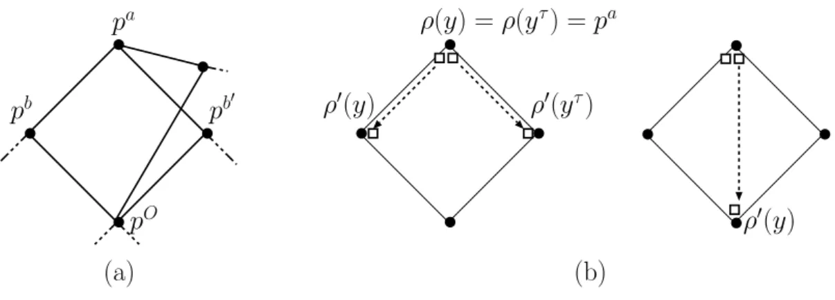
We endowΓ with two orientations. Theforward orientationof Γ is an orientation such that p^s are sinks and p^O is the unique source. The backward orientation of Γ is the reverse of the forward orientation. See Figure 2. For a potential ρ, a potential ρ⁰ is called a forward neighbor to ρ if for x ∈ V G with ρ(x) 6= ρ⁰(x),

−−−−−−→

ρ(x)ρ⁰(x) is an edge of the forward orientation, or (ρ(x), ρ⁰(x)) = (p^O, p^s) for some s ∈ S. Similarly, a potential ρ⁰ is called a backward neighbor to ρ if for

x ∈ V G with ρ(x) 6= ρ⁰(x), −−−−−−→

ρ(x)ρ⁰(x) is an edge of the backward orientation, or (ρ(x), ρ⁰(x)) = (p^s, p^O) for some s ∈ S. A potential ρ⁰ is called a neighbor to ρ if ρ⁰ is a forward neighbor or a backward neighbor to ρ. We give an optimality criterion to (2.4) using the notion of neighbors as follows.

Proposition 2.3. A potential ρ is optimal to (2.4)if and only if hc, d^ρi ≤ hc, d^ρ0i

holds for every neighbor ρ⁰ to ρ.

Namely, if ρ is not optimal, there is another potential ρ⁰ close to ρ such that hc, d^ρi>hc, d^ρ0i.

2.4 Euler condition

Recall that a graph (G, c) is calledinner Eulerianif cis integral and the degree of each inner node is even.

Lemma 2.4. For an inner Eulerian graph (G, c) and two potentials ρ, ρ⁰, we have hc, d^ρ0i − hc, d^ρi ∈2Z.

Proof. Since (G, c) is inner Eulerian,c∈Z^EG₊ can be decomposed into the sum of the characteristic vectors of cycles C_i and S-paths P_j. Then we have

hc, d^ρ0i − hc, d^ρi=∑

i

{d^ρ0(Ci)−d^ρ(Ci)}+∑

j

{d^ρ0(Pj)−d^ρ(Pj)}= 0 mod 2,

where d^ρ0(Ci) = d^ρ(Ci) mod 2 and d^ρ0(Pj) = d^ρ(Pj) mod 2 follow from the bi- partiteness of Γ.

2.5 Reducing the feasibility problem for K

+ K

to the maximization problem for K

Here we describe a reduction of the multiflow feasibility problem forH =K₃+K₃ toK_3,3-metric-weighted maximum multiflow problem (2.2).

LetGbe a graph with capacityc. LetH = (S, R) be the demand graph defined byS={s₁, s₂, s₃, t₁, t₂, t₃}andR ={s_is_j}1≤i<j≤3∪ {t_it_j}1≤i<j≤3, andq :R→R₊ a demand function. Construct a new graph (G⁰, c⁰) from (G, c) by adding new terminals S⁰ = {a1, a2, a3, b1, b2, b3} with A = {a1, a2, a3}, B = {b1, b2, b3} and connecting a_i and s_i by an edge with capacityq(s_is_j) +q(s_is_k) and connecting b_i and t_i by an edge with capacity q(t_it_j) +q(t_it_k) (i = 1,2,3;{i, j, k} = {1,2,3}).

Then (G⁰, c⁰) is inner Eulerian with respect to S⁰ if (G, c;H, q) satisfies the Euler condition. Consider (2.2) for (G⁰, c⁰;S⁰, µ_A,B). Let ρ^∗ be a potential defined by

(2.9) ρ^∗(x) =

{ p^x if x∈S⁰,

p^O otherwise, (x∈V G).

Then we have the following.

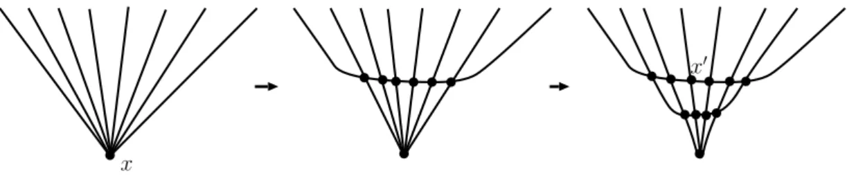
x

x⁰

Figure 3: Reduction of an inner node

Lemma 2.5. The multiflow feasibility problem for(G, c;H, q)is feasible if and only if potential ρ^∗ defined by (2.9) is optimal to (2.4) for (G⁰, c⁰;S⁰, µ_A,B). Moreover, if feasible, then the restriction of any optimal multiflow f^∗ to (G, c;S)is a feasible multiflow.

Proof. Suppose that (G, c;H, q) is feasible. From a feasible multiflow f = (P, λ), we can construct an optimal multiflow as follows. For each path P ∈ P, if the ends of P are s_i and s_j (resp. t_i and t_j), then extend P by adding edges a_is_i and s_ja_j (resp. b_it_i and t_jb_j). Let f⁰ be the resulting multiflow to (G⁰, c⁰;S⁰). By construction, a_is_i and b_it_i for i = 1,2,3 are saturated by f⁰. Clearly f⁰ and ρ^∗ satisfies the optimality criterion I (Lemma 2.2).

Conversely, suppose that ρ^∗ is optimal. Take an optimal multiflow f^∗. Then edges s_ia_i and t_ib_i for i= 1,2,3 are saturated by f^∗. By (2.8), each path passing s_ia_i is necessarily an (a_i,{a_j, a_k})-path, and each path passingt_ib_i is necessarily a (b_i,{b_j, b_k})-path. Then f^∗ consists of (a_i, a_j)-paths of the total flow-value q(s_is_j) for 1≤i < j ≤3 and (b_i, b_j)-paths of the total flow-valueq(t_it_j) for 1≤i < j ≤3.

Restricting f^∗ to (G, c;S), we obtain a feasible multiflow.

Therefore Theorem 1.4 implies Theorem 1.3.

2.6 Making each inner node have degree four

Here we describe a standard method reducing (2.2) to the problem on a graph with small-degree; see [3, p. 50] for example. Suppose that (G, c) is inner Eulerian. By multiplying edges, we can make each edge have unit capacity. Take an inner node x ∈ V G of degree greater than 4. Transform (G, c) into (G⁰, c⁰) by changing the incidence atx as in Figure 3.

Then we can easily see that any 1/k-integral multiflow in (G⁰, c⁰) can be trans- formed into a 1/k-integral multiflow in (G, c) having the same objective value, and any 1/k-integral multiflow in (G, c) can also be transformed into a 1/k-integral multiflow in (G⁰, c⁰) having the same objective value. Furthermore,

(2.10) any optimal potentialρ for (G, c) is extended to an optimal potential ρfor (G⁰, c⁰) by settingρ(x⁰) := ρ(x) for each new node x⁰ in (G⁰, c⁰), which is an easy consequence of the optimality criterion I (Lemma 2.2).

2.7 proof

The combinatorial duality theorem (Theorem 2.1) was essentially given in [12, p. 241] as a corollary of Karzanov’s modular closure construction together with the orbit splitting method. Here, we describe a more direct geometric proof by calculating the explicit coordinate of the tight span of µA,B. This approach is suitable to prove the optimality criterion II (Proposition 2.3).

2.7.1 T-dual to µ-problem

We start with a general framework. Letµbe a metric defined on the terminals S.

The µ-weighted maximum multiflow problem (for short, µ-problem) is:

(2.11) Maximize ∑

P∈P

µ(s_P, t_P)λ(P) over all multiflows f = (P, λ) in (G, c), wheres_P and t_P are the ends of P. As is well-known in the multiflow theory [14], the LP-dual toµ-problem (2.11) is given as follows:

Minimize ∑

e∈EG

c(e)d(e) (2.12)

subject to d: metric onV G,

d(s, t) =µ(s, t) (s, t∈S).

Sincecis nonnegative, we can always take an optimal metric from theminimal set of the feasible region of (2.12). Such a minimal metric is called a tight extension ofµ. Now let us introduce the formal definitions below. A metricd onV is called an extension of a metric µ on S if S ⊆ V and d(s, t) = µ(s, t) for s, t ∈ S. An extensiond onV of µ is said to betight if there is no extension d⁰ on V of µ with d⁰ ≤d andd⁰ 6=d. Therefore (2.12) might be regarded as the problem of finding a tight extension d onV G of µwith hc, di minimum.

Isbell [7] and Dress [1] independently showed that for any metric µthere is an essentially uniqueuniversaltight extension of µsuch that every tight extension of µ is a subspace of it. We shall describe it. For a metric µ on S, we define two polyhedral sets P_µ and T_µ in R^S₊ by

P_µ = {p∈R^S |p(s) +p(t)≥µ(s, t) (s, t∈S)}, (2.13)

Tµ = the set of minimal elements of Pµ.

T_µ is called thetight span ofµ. Fors∈S, letµ_s ∈R^S be a point inT_µ defined by µ_s(t) =µ(s, t) (t ∈S).

Namely, µ_s is thes-th row vector of distance matrix µ. One can easily see that kµ_s−µ_tk∞=µ(s, t) (s, t∈S).

Thereforeµis isometrically embedded into (T_µ, l_∞), and thus (T_µ, l_∞) is regarded as an extension ofµ. Moreover, every tight extension ofµis embedded into (T_µ, l_∞) as follows.

Theorem 2.6 ([7, 1]). (T_µ, l_∞) is a tight extension of µ. Moreover, for any tight extension d on V of µ, there is a unique map ρ:V →T_µ such that

(i) ρ(s) =µ_s for s∈S, and

(ii) kρ(x)−ρ(y)k_∞ =µ(x, y) for x, y ∈V.

In particular, the map ρ is given explicitly as (ρ(x))(s) =d(x, s) for x∈V, s ∈S.

Consider the following continuous location problem on (T_µ, l_∞).

Minimize ∑

e=xy∈EG

c(e)kρ(x)−ρ(y)k∞

(2.14)

subject to ρ:V G→T_µ (x∈V G), ρ(s) =µ_s (s∈S).

We call it T-dual; see also [4] for a general version. By the previous theorem, we have a sharper duality theorem for µ-problem:

Corollary 2.7. The maximum value of µ-problem (2.11) is equal to the minimum value of T-dual (2.14).

A map ρ : V G → T_µ satisfying the constraint of T-dual is called a potential.

The relationship between LP-dual (2.12) andT-dual (2.14) is summarized as fol- lows:

(2.15) (i) For a metricdminimalin the feasible region of LP-dual (2.12), a map ρ^d :V G→R^S defined by

ρ^d(x)(s) = d(s, x) (s∈S, x∈V G) is a potential to (2.14).

(ii) For a potential ρ to (2.14), a metric d^ρ defined by d^ρ(x, y) = kρ(x)−ρ(y)k∞ (x, y ∈V G) is minimal in the feasible region to LP-dual (2.12).

In particular, we can always take an optimal solution d^ρ of the LP-dual for some potential ρ:V G→T_µ of T-dual.

2.7.2 The tight span for µ_A,B

Letµ_A,B be the metric defined by (2.1). Let us calculate T_µA,B explicitly. Let q^O, q^a (a ∈A),q^b (b∈B) be the points in T_µA,B defined by

q^O = 2χ_S,

q^a = q^O+ 2(−χ_a+χ_¯a) = (µ_A,B)_a, q^b = q^O+ 2(−χ_b+χ¯b) = (µ_A,B)_b. Recall ¯a=A\a and ¯b=B\b. Then we have:

q

q

q

q

(a) (b)

Figure 4: (a) T_µA,B and (b)L¹∩T_µA,B with graphΓ¹ Lemma 2.8. T_µA,B coincides with

(2.16) ∪

(a,b)∈A×B

convex hull of {q^O, q^a, q^b}.

Proof. For a general metricµ, a point p∈P_µ is minimal inP_µ (i.e.,p∈T_µ) if and only if p−²χs 6∈Pµ for any ² > 0 and s ∈S. From this, to see (2.16) ⊆ Tµ_A,B is straightforward. We show the converse. Takep∈T_µA,B. By (2.13), there isa⁰ ∈A withp(a⁰)≥2. By minimality, there isa∈A\a⁰withp(a⁰)+p(a) = µ_A,B(a⁰, a) = 4.

In particular, p(a) ≤ 2. Again we have p(a⁰⁰) ≥ p(a) for a⁰⁰ ∈ A \ {a, a⁰} by p(a) +p(a⁰⁰) ≥ 4. By minimality, p(a⁰⁰) = p(a⁰) holds. Similarly, there is b ∈ B such thatp(b)≤2 and p(b⁰) = p(b⁰⁰)≥2 for b⁰, b⁰⁰∈B \b. Then we have

q^O =p−(2−p(a))(−χ_a+χ_a¯)−(2−p(b))(−χ_b+χ¯b).

By calculation, we have p=

(p(a) +p(b)

2 −1

)

q^O+ 2−p(a)

2 q^a+2−p(b) 2 q^b. Since p(a) +p(b)≥µ_A,B(a, b) = 2, all coefficients are nonnegative.

Therefore Tµ_A,B is isomorphic to the join of one point q^O and the complete bipartite graph with bipartition{{q^a}a∈A,{q^b}b∈B}; see Figure 4 (a).

2.7.3 Drawing graphs Γ^k on T_µA,B

Here we draw the graphΓ onTµ_A,B. For a positive integer k, letL^k be the lattice (a discrete subgroup) inR^S defined by

L^k ={p∈R^S |p(s) +p(t)∈2Z/k (s, t∈S)}.

LetΓ^k be a graph whose vertices areL^k∩T_µA,B and edges are given as pq∈EΓ^k

⇔ kp−qk_∞= 1/k. Then L¹ ∩T_µA,B consists of q^O, q^s (s∈S), and q^ab :=q^O+ (−χ_a+χ_¯a) + (−χ_b+χ¯b) ((a, b)∈A×B).

(a) (b) (c) q^a

q^a0

q^b0 q^b

Figure 5: (a) an apartment, (b)L⁵∩TµA,B withΓ⁵ on an apartment, and (c) orbit O₃

In particular,Γ¹ is isomorphic toΓ by the natural correspondenceq7→p, and thus we can identify a potentialρ of (2.4) with a potentialρof T-dual (2.14) satisfying ρ(V G)⊆T_µ∩L¹; see Figure 4 (b).

For (a, b),(a⁰, b⁰)∈A×B with a6=a⁰ andb 6=b⁰, consider the following subset of T_µA,B:

∪

(u,v)∈{a,a⁰}×{b,b⁰}

convex hull of {q^O, q^u, q^v}.

We call it the (a, b, a⁰, b⁰)-apartment; the name stems from the building theory. We easily see the following properties of apartments:

(2.17) (i) For every pair p, q ∈ T_µA,B, there is an apartment containing both p and q.

(ii) Each apartment is a geodesic subspace of (TµA,B, l_∞), i.e., each pair of points p, q in the apartment has a path of length kp−qk∞ within it.

(iii) The projection of the (a, b, a⁰, b⁰)-apartment to (R^{a,b}, l_∞) is an injec- tive isometry, and its image is a square with edge length 2.

See Figure 5 (a). Recall the well-known fact that thel_∞-plane is isomorphic to the l₁-plane by 45-degree rotation. Viewing from the rotated plane, the subgraph ofΓ^k induced by the apartment is exactly the grid graph of size (2k,2k); see Figure 5 (b).

By these observations, we see that the graph Γ^k realizes the l_∞-distances among L^k∩T_µA,B as follows.

(2.18) kp−qk_∞= 1

kdist_Γ^k(p, q) (p, q ∈V Γ^k =L^k∩T_µA,B).

Indeed, take an apartment containingp, q, and project it as in Figure 5. Then we can take a zig-zag shortest path in the grid graph induced by the apartment.

2.7.4 Constructing a convex combination Here we show the following statement.

(2.19) For any potential ρ : V G → L^k∩T_µA,B(= V Γ^k), the corresponding metricd^ρcan be represented as a convex combination of{d^ρi}for some potentials ρi :V G→L¹ ∩Tµ_A,B(= V Γ¹),

where the metric d^ρ for a potential ρ is defined by (2.15). This immediately yields Theorem 2.1. Indeed, for any rational potential ρ, there is k such that ρ(V G)⊆L^k∩T_µA,B since Z^S/l⊆L^2l. To prove (2.19), we use the notion of orbits and related concepts introduced by [11]. Two edgese, e⁰ ∈EΓ^kare called mates if there is a 4-cycle containingeand e⁰ as a nonadjacent pair. Two edgese, e⁰ ∈EΓ^k are called projective if there is a sequence of edges e = e₁, e₂, . . . , e_m = e⁰ such that ei and ei+1 are mates. The projectiveness defines an equivalence relation on the set of edges EΓ^k. An equivalence class is called an orbit. Γ^k has k orbits {O₁, O₂, . . . , O_k}. Here we order O₁, O₂, . . . , O_k so that

(2.20) O_i is the orbit containing the edge connecting k−i+ 1

k q^O+ i−1

k q^ab and k−i

k q^O+ i kq^ab.

For an orbitO_i, the orbit graph Γ_i^k is the graph obtained by contracting all edges not in O_i and deleting multiple edges appeared. Then the orbit graph Γ_i^k is isomorphic to Γ¹ =Γ. This construction naturally gives a map φ_i :L^k∩T_µA,B → L¹ ∩T_µA,B by defining φ_i(p) to be the contracted point and identifying Γ_i^k with Γ¹ so that φ_i is identity on L¹ ∩T_µA,B. In particular, if ρ : V G → L^k ∩T_µA,B is a potential, then the composition φ_i ◦ρ is also a potential by φ_i(q^s) = q^s. By considering each shortest path in some apartment, we easily see that the following relation holds:

dist_Γ^k(p, q) =

∑k i=1

dist_Γ¹(φ_i(p), φ_i(q)) (p, q ∈V Γ^k).

This can also be derived from a general property of orbits in the modular graph [12].

By (2.18), for any x, y ∈V G, we have d^ρ(x, y) = kρ(x)−ρ(y)k∞= 1

kdist_Γk(ρ(x), ρ(y)) (2.21)

= 1

k

∑k i=1

dist_Γ¹(φ_i◦ρ(x), φ_i◦ρ(y)) = 1 k

∑k i=1

d^φi◦ρ(x, y).

Then we obtain a desired convex combination.

2.7.5 Proof of Proposition 2.3

Take a potential ρ :V G → V Γ in (2.4). We can identify V Γ with L¹∩Tµ_A,B by the argument above, and thus we regard ρ as V G →L¹ ∩T_µA,B. Suppose that ρ is not optimal. Thend^ρ is not optimal to (2.12). By convexity, there is a rational metricd⁰ sufficiently close to d^ρ such that

(a) (b) (c)

Figure 6: Perturbation tod^ρ (i) d⁰ is minimal in the feasible region of (2.12), (ii) hc, d⁰i<hc, d^ρi,

(iii) |d^ρ(x, y)−d⁰(x, y)|<1/2 for anyx, y ∈V G.

The property (iii) means that d⁰ is sufficiently close to d^ρ. By (i) and the corre- spondence (2.15), there uniquely exists ρ⁰ :V G→T_µA,B such that d⁰ =d^ρ0. Since d^ρ0 is rational, there is a positive even integerk such thatρ⁰(V G)⊆L^k∩T_µA,B. By (2.21), we can decomposed^ρ0 asd^ρ0 = 1/k∑k

i=1d^φi◦ρ0.By (ii), at least one ofd^φi◦ρ0 satisfies hc, d^φi◦ρ0i < hc, d^ρi. By (iii) and (2.15), we have kρ(x)−ρ⁰(x)k∞ < 1/2.

Therefore, by (2.20) and by the construction of φ_i, if 1≤ i ≤k/2, then φ_i◦ρ⁰ is a forward neighbor to ρ, and if k/2 < i≤ k, then φ_i ◦ρ⁰ is a backward neighbor to ρ. Thus we are done. Figure 6 illustrates this situation restricted to some apartment. In this figure, a small square box representsρ⁰(x), which is sufficiently close to ρ(x) that belongs to L¹∩T_µA,B represented by black dot points. Consider orbit O_i, which is represented by bold lines in (b) for 1 ≤ i ≤k/2 and in (c) for k/2< i≤k. Then (φ_i◦ρ⁰)(x)6=ρ(x) if and only if a shortest path between ρ⁰(x) and ρ(x) crosses O_i. In (b), the change fromρ(x) to (φ_i◦ρ⁰)(x) produced by such a crossing is one of p^O→p^ab, p^O→p^a,p^O →p^b,p^ab →p^a, and p^ab →p^b for some a, b. This implies that φ_i ◦ρ⁰ for 1 ≤ i ≤ k/2 is a forward neighbor. In (c), the change occurs in the reverse way, which implies that φ_i ◦ρ⁰ for k/2 < i ≤ k is a backward neighbor.

3 Fractional splitting-off

Let (G, c) be an integer-capacitated graph (allowing multiple edges and loops).

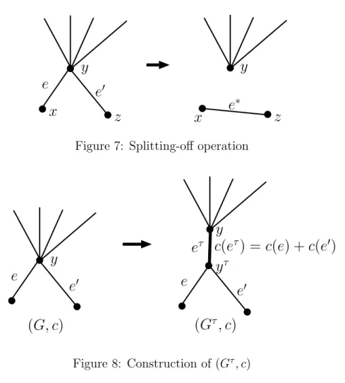
We begin with some notation. For two consecutive edges e and e⁰ incident to y, a triple (e, y, e⁰) is called a fork. If both e and e⁰ have no multiple edge and e =xy and e⁰ =yz, then (e, y, e⁰) is also simply denoted by xyz. For a fork τ = (e, y, e⁰), the splitting-off operation at τ is to decrease the capacity of edges e, e⁰ by one, and add a new edge e^∗ connecting the end of e and e⁰ different from y with unit capacity; see Figure 7. If this operation keeps the optimal value ν(G, c) invariant,

y

e e

x z

y

x z

e

Figure 7: Splitting-off operation

y e

e

y

e e

c(e

) = c(e) + c(e

) y

(G, c) (G

, c)

e

Figure 8: Construction of (G^τ, c)

then we say that τ is splittable. In addition, if the new graph has a 1/k-integral optimal multiflow, then so does the original graph. Consequently, if we can succeed the splitting-off operations until there is no inner node, then the resulting graph clearly has an integral optimal multiflow (by metricity of µ_A,B), and so does the original graph.

As seen in the introduction, our problem (2.2) may have no integral optimal solution. So we consider a fractional variant of the splitting-off operation. Our approach is slightly different from Karzanov’s one in [8, 13]. For a forkτ = (e, y, e⁰) withe=xyande⁰ =yz, consider the graph (G^τ, c) obtained from (G, c) by adding a new node y^τ and a new edge e^τ = yy^τ and reconnecting e and e⁰ to y^τ. The capacity of e^τ is defined by c(e) +c(e⁰); see Figure 8. Then multiflows in (G, c) and in (G^τ, c) are in one-to-one correspondence as follows.

(3.1) (i) For a multiflow f = (P, λ) in (G^τ, c), contract e^τ (to y) for each path inP(e^τ). Then the resulting f is a multiflow to (G, c).

(ii) For a multiflow f = (P, λ) in (G, c), replace subpath (x, e, y) of each path in P(e)\ P(e⁰) by (x, e, y^τ, e^τ, y), replace subpath (z, e⁰, y) of each path in P(e⁰) \ P(e) by (z, e⁰, y^τ, e^τ, y), and replace subpath (x, e, y, e⁰, z) of each path in P(e, e⁰) by (x, e, y^τ, e⁰, z). Then the re- sultingf is a multiflow in (G^τ, c).

We shall often identify a multiflow for (G, c) with a multiflow for (G^τ, c) by this