1804
INVITED SURVEY PAPER
A Comprehensive Survey of Potential Game Approaches to Wireless Networks
Koji YAMAMOTO†a),Senior Member
SUMMARY Potential games form a class of non-cooperative games where the convergent of unilateral improvement dynamics is guaranteed in many practical cases. The potential game approach has been applied to a wide range of wireless network problems, particularly to a variety of chan- nel assignment problems. In this paper, the properties of potential games are introduced, and games in wireless networks that have been proven to be potential games are comprehensively discussed.
key words: potential game, game theory, radio resource management, channel assignment, transmission power control
1. Introduction
The broadcast nature of wireless transmissions causes co- channel interference and channel contention, which can be viewed as interactions among transceivers. Interactions among multiple decision makers can be formulated and an- alyzed using a branch of applied mathematics called game theory[61],[131]. Game-theoretic approaches have been applied to a wide range of wireless communication tech- nologies, including transmission power control for code di- vision multiple access (CDMA) cellular systems[153]and cognitive radios[132]. For a summary of game-theoretic ap- proaches to wireless networks, we refer the interested reader to[68],[91],[92],[108], [168]. Application-specific sur- veys of cognitive radios and sensor networks can be found in[64],[102],[160],[166],[178],[189].
In this paper, we focus on potential games[126], which form a class of strategic form games with the following de- sirable properties:
• The existence of a Nash equilibrium in potential games is guaranteed in many practical situations[126](The- orems 1 and 2 in this paper), but is not guaranteed for general strategic form games. Other classes of games possessing Nash equilibria are summarized in [92,§2.2] and[68,§3.4].
• Unilateral improvement dynamics in potential games with finite strategy sets is guaranteed to converge to the Nash equilibrium in a finite number of steps, i.e., they do not cycle[126](Theorem 4 in this paper). As a result, learning algorithms can be systematically de- signed.
A game that does not have these properties is discussed in Manuscript received February 12, 2015.
Manuscript revised May 15, 2015.
†The author is with the Graduate School of Informatics, Kyoto University, Kyoto-shi, 606-8501 Japan.
a) E-mail: [email protected] DOI: 10.1587/transcom.E98.B.1804
Example 2 in Sect. 2.
We provide an overview of problems in wireless net- works that can be formulated in terms of potential games.
We also clarify the relations among games, and provide sim- pler proofs of some known results. Problem-specific learn- ing algorithms[92],[168]are beyond the scope of this pa- per.
The remainder of this paper is organized as follows: In Sect. 2, 3, and 4, we introduce strategic form games, poten- tial games, and learning algorithms, respectively. We then discuss various potential games in Sects. 5 to 18, as shown in Table 1. Finally, we provide a few concluding remarks in Sect. 19.
The notation used here is shown in Table 2. Unless the context indicates otherwise, sets of strategies are denoted by calligraphic uppercase letters, e.g.,Ai, strategies are de- noted by lowercase letters, e.g.,ai∈ Ai, and tuples of strate- gies are denoted by boldface lowercase letters, e.g.,a. Note thataiis a scalar variable whenAiis a set of scalars or in- dices,aiis a vector variable whenAiis a set of vectors, and aiis a set variable whenAiis a collection of sets.
We useRto denote the set of real numbers,R+to de- note the set of nonnegative real numbers,R++to denote the set of positive real numbers, andCto denote the set of com- plex numbers. The cardinality of setAis denoted by|A|.
The power set ofAis denoted by 2A. Finally,½conditionis the indicator function, which is one whenconditionis true and is zero otherwise.
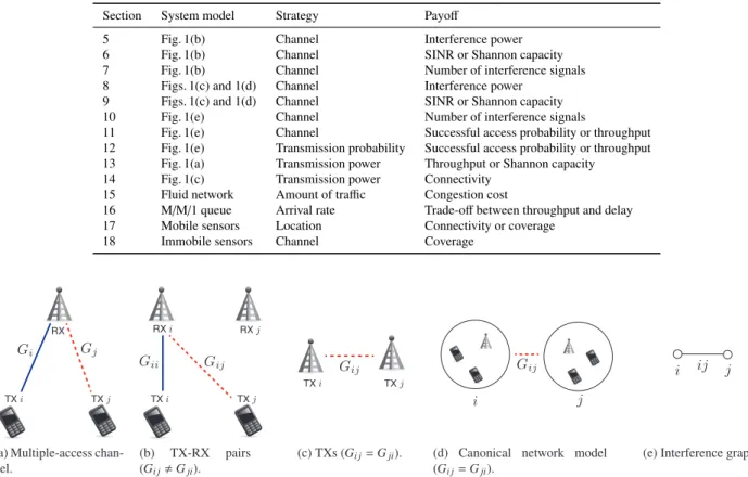
We treat many system models, as shown in Fig. 1. In multiple-access channels, as shown in Fig. 1(a), multiple transmitters (TXs/users/mobile stations/terminals) transmit signals to a single receiver (RX/base station (BS)/access point (AP)). In Fig. 1(a),Gi represents the link gain from TXito the RX.
In a network model consisting of TX-RX pairs, as shown in Fig. 1(b), each TX i transmits signals to RX i. In this case, Gi j Gji. In a network model consisting of TXs shown in Fig. 1(c), each TX (BS/AP/transceiver/station/terminal/node) interferes with others. In this model, Gi j = Gji. A “canonical network model”[15], shown in Fig. 1(d), consists of clusters that are spatially separated in order forGi j =Gjito hold. Note that these network models have been discussed in terms of graph structure in[143].
We use jito denote a directed link from TXito TX j or clusterito cluster j. Let interference graph (I,E) be an undirected graph, where the set of verticesI = {1,2, . . .} Copyright c2015 The Institute of Electronics, Information and Communication Engineers
Table 1 Games discussed in this paper.
Section System model Strategy Payoff
5 Fig. 1(b) Channel Interference power
6 Fig. 1(b) Channel SINR or Shannon capacity
7 Fig. 1(b) Channel Number of interference signals
8 Figs. 1(c) and 1(d) Channel Interference power
9 Figs. 1(c) and 1(d) Channel SINR or Shannon capacity
10 Fig. 1(e) Channel Number of interference signals
11 Fig. 1(e) Channel Successful access probability or throughput
12 Fig. 1(e) Transmission probability Successful access probability or throughput 13 Fig. 1(a) Transmission power Throughput or Shannon capacity
14 Fig. 1(c) Transmission power Connectivity
15 Fluid network Amount of traffic Congestion cost
16 M/M/1 queue Arrival rate Trade-offbetween throughput and delay
17 Mobile sensors Location Connectivity or coverage
18 Immobile sensors Channel Coverage
Fig. 1 System models. Straight blue lines represent communication channels of playeriand red dashed lines represent interference channels to playeri.
corresponds to TXs or clusters, andi interferes with j if ji ∈ E, as shown in Fig. 1(e), i.e., E {ji | GjiP > T} wherePis the transmission power level for every TX andT is a threshold of the received power. Note that in undirected graph (I,E), ji ∈ E ⇔ i j ∈ E, for every{i,j} ⊂ I. We denote the neighborhood ofiin graph (I,E) byIi {j∈ I \ {i} | ji∈ E }. We also defineIcii(c){j∈ Ii|cj=ci}, then,|Icii(c)|=
j∈Ii½cj=ci =
ji½cj=ci½i j∈E. 2. Game-Theoretic Framework
We begin with the definition of a strategic form game and present an example of a game-theoretic formulation of a simple channel selection problem. Moreover, we discuss other useful concepts, such as the best response and Nash equilibrium. The analysis of Nash equilibria in the channel selection example reveals the potential presence of cycles in best-response adjustments.
Definition 1: Astrategic (or normal) form gameis a triplet G (I,(Ai)i∈I,(ui)i∈I), or simply G (I,(Ai),(ui)), whereI={1,2, . . . ,|I|}is a finite set ofplayers(decision makers)†,Ai is the set ofstrategies(or actions) for player
†Infinite player (or non-atomic) potential games introduced in [150],[151] are beyond the scope of this paper. Infinite player potential games have been applied to BS selection games[158], [170].
i∈ I, andui:
i∈IAi → Ris thepayoff (or utility) func- tion of playeri∈ Ithat must be maximized.
If S ⊆ I, we denote the Cartesian product
i∈SAi
by AS. If S = I, we simply write A to denote AI, and
i to denote
i∈I. When S = I \ {i}, we let A−i
denote AI\{i}, and
ji denote
j∈I\{i}. For ai ∈ Ai, aS =(ai)i∈S ∈ AS, a =(ai,a−i) =(a1, . . . ,a|I|) ∈ A, and a−i=(a1, . . . ,ai−1,ai+1, . . . ,a|I|)∈ A−i.
Example 1: Consider a channel selection problem in the TX-RX pair model shown in Fig. 1(b). Each TX-RX pair is assumed to select its channel in a decentralized manner in order to minimize the received interference power.
The channel selection problem can be formulated as a strategic form game G1 (I,(Ci),(u1i)). The elements of the game are as follows: the set of players Iis the set of TX-RX pairs. The strategy set for each pairi,Ci is the set of available channels. The received interference power at RX i ∈ Iis determined by a combination of channels c=(ci)i∈I∈ C=
iCi, where Ii(c)
ji
Gi jP½cj=ci. (1) Let−Ii(c) be the payofffunction to be maximized, i.e.,
u1i(c)−Ii(c)=−
ji
Gi jP½cj=ci. (2)
1806
Table 2 Notation.
G Strategic form game
I Finite set of players,I={1,2, . . . ,|I|}
If(a) {i∈ I |f∈ai}
Ai Set of strategies for playeri∈ I A Strategy space,
i∈IAi
ui Payofffunction for playeri∈ I φ Potential function
BRi Best-response correspondence of playeri ai Strategy of playeri,ai∈ Ai
Δ(Ai) Set of probability distributions overAi
xi Mixed strategy,xi∈Δ(Ai) x Mixed strategy profile,x∈
iΔ(Ai)
Gi Link gain between TX i and a single isolated RX in Fig. 1(a)
Gi j Link gain between TXjand RXi;GjiGi jin Fig. 1(b), andGji=Gi jin Figs. 1(c) and 1(d)
ji Directed link fromitoj E Set of edges in undirected graph
Ii {j∈ I \ {i} |ji∈ E }. Neighborhood in graph (I,E) Icii(c) {j∈ Ii|cj=ci}.
N Common noise power for every player Ni Noise power at RXi
Ni(ci) Noise power at RXiin channelci
Ii(c) Interference power at RXiat channel arrangementc Ci Set of available channels for playeri
ci(∈ Ci) Channel of playeri c (ci)i∈I∈
iCi
Pi Set of available transmission power levels for playeri pi(∈ Pi) Transmission power level of playerias a strategy
p (pi)i∈I∈
iPi
P Identical transmission power level for every player Pi Transmission power level for playerias a constant Γ Required signal-to-interference-plus-noise power ratio
(SINR)
Note thatG1 was introduced in[140], and we further discuss it in Example 2.
Definition 2: Thebest-response correspondence†(or sim- ply, best response) BRi:A−i → 2Ai of playerito strategy profilea−iis the correspondence
BRi(a−i)
{ai∈ Ai|ui(ai,a−i)≥ui(ai,a−i),∀ai ∈ Ai}, (3) or equivalently, BRi(a−i)arg maxai∈Aiui(ai,a−i).
A fundamental solution concept for strategic form games is the Nash equilibrium:
Definition 3: A strategy profile a∗ = (a∗i,a∗−i) ∈ A is a pure-strategyNash equilibrium (or simply a Nash equilib- rium) of game (I,(Ai),(ui)) if
ui(a∗i,a∗−i)≥ui(ai,a∗−i), (4) for everyi ∈ Iandai ∈ Ai; equivalently,a∗i ∈ BRi(a∗−i) for everyi∈ I. That is,a∗i is a solution to the optimization problem maxai∈Aiui(ai,a∗−i).
†A correspondence is a set-valued function for which all image sets are non-empty, e.g,[92],[131].
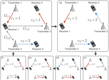
Fig. 2 Arrangement used in Example 2. A cycle results from the best- response adjustment.
At the Nash equilibrium, no player can improve his/her payoffby adopting a different strategyunilaterally; thus, no player has an incentive to unilaterally deviate from the equi- librium. The Nash equilibrium is a proper solution concept;
however, the existence of a pure-strategy Nash equilibrium is not necessarily guaranteed, as shown in the next example.
Example 2: Consider G1 and the arrangement shown in Fig. 2, i.e.,I={1,2,3},Ci = {1,2}for everyi, andG13 >
G12,G21 >G23, andG32>G31††. The game does not have a Nash equilibrium, i.e., for every channel allocation, at least one pair has an incentive to change his/her channel. The de- tails are as follows: when all players choose the same chan- nel, e.g., (c1,c2,c3)=(1,1,1), every player has an incentive to change his/her channel because BRi(c−i) = {2}for alli;
thus, it is not in Nash equilibrium. On the contrary, when two players choose the same channel, and the third player chooses a different channel, e.g., (c1,c2,c3) = (1,1,2), as shown in Fig. 2(a), BR2(c−2)={2}, i.e., pair 2 has an incen- tive to change its channela2 from 1 to 2, and (4) does not hold. Because of the symmetry property of the arrangement in Fig. 2, every strategy profile does not satisfy (4). Fur- thermore, the best-response channel adjustments, which will be formally discussed in Sect. 4, cycle as (1,1,2), (1,2,2), (1,2,1), (2,2,1), (2,1,1), (2,1,2), and (1,1,2), as shown in Figs. 2(a-f).
The channel allocation game G1 is discussed further in Sect. 5.
3. Potential Games
We state key definitions and properties of potential games in Sect. 3.1, show how to identify and design exact poten- tial games in Sects. 3.2 and 3.3, and show how to identify ordinal potential games in Sect. 3.4.
††This setting is essentially the same as that used in[63],[121], [134, Example 4.17],[137].
3.1 Definitions and Properties of Potential Games Monderer and Shapley [126] introduced the following classes of potential games†:
Definition 4: A strategic form game (I,(Ai),(ui)) is anex- act potential game(EPG) if there exists anexact potential functionφ:A →Rsuch that
ui(ai,a−i)−ui(ai,a−i)=φ(ai,a−i)−φ(ai,a−i), (5) for everyi∈ I,ai,ai∈ Ai, anda−i∈ A−i.
Definition 5: A strategic form game (I,(Ai),(ui)) is a weighted potential game (WPG) if there exist aweighted potential functionφ:A →Rand a set of positive numbers {αi}i∈Isuch that
ui(ai,a−i)−ui(ai,a−i)=αi(φ(ai,a−i)−φ(ai,a−i)), (6) for everyi∈ I,ai,ai∈ Ai, anda−i∈ A−i.
Definition 6: A strategic form game (I,(Ai),(ui)) is anor- dinal potential game(OPG) if there exists anordinal poten- tial functionφ:A →Rsuch that
sgn(ui(ai,a−i)−ui(ai,a−i))
=sgn(φ(ai,a−i)−φ(ai,a−i)), (7) for everyi ∈ I,ai,ai ∈ Ai, anda−i ∈ A−i, where sgn(·) denotes the sign function.
Although the potential functionφis independent of the indices of the players,φreflects any unilateral change in any payofffunctionuifor every playeri.
Since an EPG is a WPG and a WPG is an OPG [126],[177], the following properties of OPGs are satisfied by EPGs and WPGs.
Theorem 1(Existence in finite OPGs): Every OPG with finite strategy sets possesses at least one Nash equilibrium [126, Corollary 2.2].
Theorem 2(Existence in infinite OPGs): In the case of in- finite strategy sets, every OPG with compact strategy sets and continuous payofffunctions possesses at least one Nash equilibrium[126, Lemma 4.3].
Theorem 3(Uniqueness): Every OPG with a compact and convex strategy space, and a strictly concave and contin- uously differentiable potential function possesses a unique Nash equilibrium[138, Theorem 2],[154].
The most important property of potential games is acyclicity, which is also referred to as the finite improve- ment property.
†There are a variety of generalized concepts of potential games, e.g., generalized ordinal potential games [126], best- response potential games[177], pseudo-potential games[56], near- potential games[30],[31], and state-based potential games[117].
Applications of these games are beyond the scope of this paper.
Definition 7(Finite improvement property[126]): A path in (I,(Ai),(ui)) is a sequence (a[0],a[1], . . .) such that for every integer k ≥ 1, there exists a unique player i such that ai[k] ai[k−1] ∈ Ai while a−i[k] = a−i[k−1].
(a[0],a[1], . . .) is animprovement pathif, for everyk≥ 1, ui(a[k])>ui(a[k−1]), whereiis the unique deviator at step k. (I,(Ai),(ui)) has thefinite improvement property (FIP)if every improvement path is finite.
Theorem 4: Every OPG with finite strategy sets has the FIP[126, Lemma 2.3]; that is, unilateral improvement dy- namics is guaranteed to converge to a Nash equilibrium in a finite number of steps.
3.2 Identification of Exact Potential Games
The definition of an EPG utilizes a potential function (5).
Sometimes, however, it is beneficial to know if a given game is an EPG independently of its potential function. The fol- lowing properties of EPGs and classes of games known to be EPGs are useful for the identification and derivation of potential functions. Note that each EPG has a unique ex- act potential function except for an additive constant[126, Lemma 2.7].
Theorem 5: Let (I,(Ai),(ui)) be a strategic form game where strategy setsAiare intervals of real numbers and pay- offfunctionsuiare twice continuously differentiable. Then, the game is an EPG if and only if
∂2ui(a)
∂ai∂aj
=∂2uj(a)
∂ai∂aj
, (8)
for everyi,j∈ I[126, Theorem 4.5].
Theorem 6: Let (I,(Ai),(ui,1)) and (I,(Ai),(ui,2)) be EPGs with potential functionsφ1(a) andφ2(a), respectively.
Furthermore, letα, β∈R. Then, (I,(Ai),(αui,1+βui,2)) is an EPG with potential functionαφ1(a)+βφ2(a)[59].
3.2.1 Coordination-Dummy Games
Ifui(a) =u(a) for alli ∈ I, whereu: A → R, the game (I,(Ai),(u)) is called acoordination game††or anidentical interest game, anduis called a coordination function[59].
Ifui(a)=di(a−i) for alli∈ I, wheredi:A−i→R, the game (I,(Ai),(di)) is called adummy game, anddiis called a dummy function[59].
Ifui(a) = si(ai) for alli ∈ I, where si:Ai → R, the game (I,(Ai),(si)) is called aself-motivated game, andsiis called a self-motivated function[133].
Theorem 7: (I,(Ai),(ui)) is an EPG if and only if there exist functionsu:A →Randdi:A−i→Rsuch that
ui(ai,a−i)=u(ai,a−i)+di(a−i), (9)
††The term “coordination game” is also used to describe games where players receive benefits when they choose the same strategy [47].
1808
for every i ∈ I [59], [163]. This game is said to be a coordination-dummy game. The potential function of this game isφ(a)=u(a).
Example 3: From Theorem 7, any identical interest game is an EPG. Almost all games found in studies applying iden- tical interest games[19],[27],[55],[74],[107],[142],[165]
have the form of gameG2(I,(Ai),(u2i)), where u2i(a)
j
fj(a), (10)
for everyi∈ Iandfj(a) is a performance indicator of player j, e.g.,fj(a) is the individual throughput andu2i(a) is the ag- gregated throughput of all players[165]. Note that in most of these works,G2 is used for comparison with other games.
Example 4: Closely related toG2, the form of gameG3 with payoff
u3i(a) fi(ai,aIi)+
j∈Ii
fj(aj,aIj), (11) where fi: Ai × AIi → R, is found in many scenarios:
data stream control in multiple-input and multiple-output (MIMO)[14], channel assignment[187], joint power, chan- nel and BS assignment[162], joint power and user schedul- ing[207], BS selection[53], and BS sleeping[210]. Note thatG3 is not an identical interest game, but can be seen as G2 on graphs, where the performance indicator of playeriis a function of strategies of its neighbors, i.e., fi:Ai× AIi → R, and the sum of the performance indicators of playeriand neighborsIiis set for the payofffunction of playeri. It can be easily proved thatG3 is an EPG with potential
φ3(a)=
i
fi(ai,aIi). (12)
3.2.2 Bilateral Symmetric Interaction Games
A strategic form gameG4 (I,(Ai),(u4i)) is called abi- lateral symmetric interaction (BSI) gameif there exist func- tionswi j:Ai× Aj→Randsi:Ai→Rsuch that
u4i(a)=
ji
wi j(ai,aj)−si(ai), (13) wherewi j(ai,aj) = wji(aj,ai) for every (ai,aj) ∈ Ai× Aj
[174].
Theorem 8([174]): A BSI gameG4 is an EPG with poten- tial function†
φ4(a)= 1 2
i
ji
wi j(ai,aj)−
i
si(ai)
=
i<j
wi j(ai,aj)−
i
si(ai). (14) Example 5: Consider a quasi-Cournot game G5
†
i<j=
{i,j}⊆I=|I|
i=1
|I|
j=i+1.
(I,(Ai),(u5i)) with a linear inverse demand function, where each playeri∈ Iproduces a homogeneous product and de- termines the output. LetAi=R++ be a set of possible out- puts. The payofffunction of playeriis defined by
u5i(a) α−β
jaj
ai−costi(ai), (15) whereα, β > 0 and costi:Ai → Ris a differentiable cost function. Since
u5i(a)=αai−βai2−costi(ai)
self-motivated function
−β
jiajai
BSI
, (16)
G5 is an EPG with potential φ5(a)=α
iai−β
iai2−
ici(ai)−β
i<jaiaj
(17) [163]. Further discussion can be found in[126],[174].
3.2.3 Interaction Potential
Theorem 9([174]): A normal form game G6 (I, (Ai),(u6i)) is an EPG if and only if there exists a function {ΦS | ΦS:AS → R,S ⊆ I }(called aninteraction poten- tial) such that
u6i(a)=
S⊆I:i∈S
ΦS(aS), (18)
for everya∈ Aandi∈ I. The potential function is
φ6(a)=
S⊆I
ΦS(aS). (19)
3.2.4 Congestion Games
In congestion games (CGs), the payofffor using a resource (e.g., a channel or a facility) is a function of the number of players using the same resource. More precisely, CGs are defined as follows:
In the congestion model proposed by Rosenthal[149], each playeriuses a subsetaiof common resourcesF, and receives resource-specific payoffwf(|If(a)|) from resource f ∈ ai according to the number of players using resource f. Here, wf: {1, . . . ,|I|} → R, If(a) {i ∈ I | f ∈ ai}represents the set of players that use resource f. Then,
|If(a)|=
i½f∈ai.
A strategic form gameG7(I,(Ai),(u7i)) associated with a congestion model, whereAi⊆2F and
u7i(a)
f∈ai
wf(|If(a)|), (20)
is called a CG. Note thatAiis a collection of subsets ofF and is not a set. Moreover, ai ∈ Ai is a set, not a scalar quantity. Note that a CG where the strategy of every player is a singleton, i.e., Ai ⊆ F and u7i(a) = wai(|Iai(a)|) is called asingleton CG.
Theorem 10: A CGG7 is an EPG with potential function
φ7(a)=
f∈∪iai
⎛⎜⎜⎜⎜⎜
⎜⎜⎝
|If(a)| k=1
wf(k)
⎞⎟⎟⎟⎟⎟
⎟⎟⎠, (21)
[126, Theorem 3.1],[149]. Furthermore, every EPG with finite strategy sets has an equivalent CG[126, Theorem 3.2].
Note that generalized CGs do not necessarily possess potential functions. For generalized CGs with potential, we refer the interested reader to[1],[120]. It was proved that CGs with player-specific payofffunctions[125], and those with resource-specific payofffunctions and player-specific constants [120], have potential. CGs with linear payoff function on undirected/directed graphs has been discussed in[20].
3.3 Design of PayoffFunctions
In some scenarios, we can design payofffunctions and as- sign them to players to ensure that the game is an EPG. Such approach is often applied in the context of cooperative con- trol[114]. These design methodologies can be used when we want to derive payofffunctions from a given global ob- jective so that the game with the designed payofffunctions is an EPG with the global objective as the potential function.
If the global objective is in the form of (19), we can derive payofffunctions by using (18).
Otherwise, we can utilize many design rules: the equally shared rule, marginal contribution, and the Shapley values[159],[174]. Since Marden and Wierman[118]have already summarized these rules, we only present marginal contribution here.
Marginal contribution, or the wonderful life utility (WLU)[182], is the following payofffunction derived from the potential function:
ui(a)=φ(a)−φ(a−i), (22) whereφ(a−i) is the value of the potential function in the ab- sence of playeri. The game with the WLU is an EPG with potential functionφ[118].
When the potential function for each player is repre- sented as the sum of functions fi: A → R, i.e., φ(a) =
j fj(a) and φ(a−i) =
ji fj(a−i), the WLU (22) can be written as
ui(a)=
j fj(a)−
ji fj(a−i)
= fi(a)−
ji(fj(a−i)−fj(a)), (23) wherefj(a−i)−fj(a) represents the loss to playerjresulting from playeri’s participation.
Example 6(Consensus game): In the consensus problem [173], each playeriadjustsaiand tries to reacha1 =a2 =
· · ·=a|I|.
Marden et al.[114]considered the global objective φ8(a)−1
2
i
j∈Ii
ai−aj, (24)
and proposed using the WLU u8i(a)−
j∈Ii
ai−aj=
ji
ai−aj½i j∈E. (25)
Since game G8 (I,(Ai),(u8i)) is a BSI game with wi j(ai,aj)=−ai−aj½i j∈E,G8 is confirmed to be an EPG.
3.4 Identification of Ordinal Potential Games
In contrast to EPGs, OPGs have many ordinal potential functions[126].
Theorem 11: Consider the game (I,(Ai),(ui)). If there exists a strictly increasing transformation fi: R → Rfor everyi∈ Isuch that game (I,(Ai),(fi(ui))) is an OPG, the original game (I,(Ai),(ui)) is an OPG with the same poten- tial function[133].
4. Learning Algorithms
A variety of learning algorithms are available to facilitate the convergence of potential games to Nash equilibrium, e.g., myopic best response, fictitious play, reinforcement learn- ing, and spatial adaptive play. Unfortunately, there is no general dynamics that is guaranteed to converge to a Nash equilibrium for a wide class of games[71]. Since Lasaulce et al.[92, Sections 5 and 6] comprehensively summarized these learning algorithms and their sufficient conditions for convergence for various classes of games (including poten- tial games), we present only two frequently used algorithms.
Definition 8: Best-response dynamicsrefers to the follow- ing update rule: At each stepk, playeri ∈ Iunilaterally changes his/her strategy fromai[k] to his/her best response a−i[k]; in particular,
ai[k+1]∈BRi(a−i[k]). (26) The other players choose the same strategy, i.e.,a−i[k+1]= a−i[k].
Note that while the term “best-response dynamics” was introduced by Matsui [119], it has many representations depending on the type of game. We also note that best- response dynamics may converge to sub-optimal Nash equi- libria. By contrast, the following spatial adaptive play can converge to the optimal Nash equilibrium. To be precise, it maximizes the potential function with arbitrarily high prob- ability.
Definition 9: Consider a game with a finite number of strategy sets.Log-linear learning[22],spatial adaptive play [198], andlogit-response dynamics[5]refer to the follow- ing update rule: At each step k, a player i ∈ I unilater- ally changes his/her strategy fromai[k] toaiwith probability xi∈Δ(Ai) according to the Boltzmann-Gibbs distribution
xi(ai|a−i[k])= exp[βui(ai,a−i[k])]
ai∈Aiexp [βui(ai,a−i[k])], (27)
1810
whereβ(0 < β < ∞) is related to the (inverse) temper- ature in an analogy to statistical physics. Note that in the limitβ→ ∞, the spatial adaptive play approaches the best- response dynamics.
Note that (27) is the solution to the following approxi- mated maximization problem:
maxai∈Ai
ui(ai,a−i)=max
xi(ai)
ai∈Ai
xi(ai)ui(ai,a−i)
≈max
xi(ai)
⎡⎢⎢⎢⎢⎢
⎢⎣
ai∈Ai
xi(ai)ui(ai,a−i)−1 β
ai∈Ai
xi(ai) logxi(ai)
⎤⎥⎥⎥⎥⎥
⎥⎦, (28) which is called a perturbed payoff, where
ai∈Aixi(ai) logxi(ai) is the entropy function. The derivation of (27) from (28) can be found in[37].
Theorem 12([22],[198]): In the finite EPG (I,(Ai),(ui)) with potential functionφ, the spatial adaptive play has the unique stationary distribution of strategy profilex∈ Δ(A), where
x(a)= exp [βφ(a)]
a∈Aexp [βφ(a)], (29)
i.e., it is also the Boltzmann-Gibbs distribution.
Further discussion can be found in[15],[116].
5. Channel Assignment to Manage Received and Gen- erated Interference Power in TX-RX Pair Model In the TX-RX pair model shown in Fig. 1(b), Nie and Co- maniciu[140]pointed out that the channel selection game G1 introduced in Sect. 2 was not an EPG. Note that the pay- offfunction ofG1 is the negated sum of received interfer- ence from neighboring TXs. To ensure that the channel se- lection game is an EPG, they considered the channel selec- tion gameG9, whose payofffunction was the negated sum of the received interference from neighboring TXs, and gen- erated interference to neighboring RXs, i.e.,
u9i(c)−
ji
(Gi jPj+GjiPi)½cj=ci. (30) Since G9 is a BSI game with wi j(ci,cj) = −(Gi jPj + GjiPi)½cj=ci, it is an EPG with potential
φ9(c)=−
i
Ii(c)=−
i
ji
Gi jPj½cj=ci, (31) which corresponds to the negated sum of received interfer- ence in the entire network. Note that in order to evaluate (30), each pairineeds to estimate or share the values of the generated interference to neighboring RXs,GjiPi½cj=ci.
Concurrently with the above, Kauffmann et al.[82]dis- cussed the following potential function φ10(c), which in- cludes RX-specific noise powerNi(ci), and derived a payoff function using Theorem 9,
φ10(c)−
i
ji
Gi jPj½cj=ci−
i
Ni(ci), (32) u10i(c)=−
ji
(Gi jPj+GjiPi)½cj=ci−Ni(ci). (33) To enable multi-channel allocation, e.g., orthogonal frequency-division multiple access (OFDMA) subcarrier al- location or resource block allocation, La et al.[88]discussed a modification ofG9 suitable for multi-channel allocation.
In contrast to unidirectional links assumed in the TX- RX pair model, Uykan and J¨antti[175],[176]discussed a channel assignment problem for bidirectional links and pro- posed a joint transmission order and channel assignment al- gorithm.
5.1 Joint Transmission Power and Channel Allocation Nie et al.[141]showed that the joint channel selection and power control game with payofffunction
u11i(p,c)−
ji
(Gi jpj+Gjipi)½ci=cj (34) is an EPG. Because the best response inG11 results in the minimum transmission power level, Bloem et al.[21]pro- posed adding termsαlog(1+Giipi)+β/pito (34) to account for the achievable data rate and consumed power. Note that these terms are self-motivated functions, and the game with the modified payofffunction is still an EPG.
As another type of joint assignment, a preliminary beamform pattern setting followed by channel allocation was discussed in[202].
5.2 Primary-Secondary Scenario and Heterogeneous Net- works
To manage interference in primary-secondary systems, Bloem et al. [21]proposed adding terms related to the re- ceived and generated interferences from and to the primary user. They also proposed adding cost terms related to pay- offfunction (34). In particular, they discussed a Stackelberg game[131], where the primary user was the leader and the secondary users were followers. Giupponi and Ibars dis- cussed overlay cognitive networks[66]and heterogeneous OFDMA networks[67]. Mustika et al.[129]took a similar approach to prioritize users.
Uplinks of heterogeneous OFDMA cellular systems with femtocells were discussed in [130], whereas down- links of OFDMA cellular systems, where each BS trans- mits to several mobile stations, were discussed in[89],[90].
OFDMA relay networks were considered in[96]. Further discussion can be found in[76]. Joint BS/AP selection and channel selection problems were discussed in[48].
6. Channel Assignment to Enhance SINR and Through- put in TX-RX Pair Model
In the TX-RX pair model shown in Fig. 1(b), the signal-to- interference-plus-noise ratio (SINR) at RXiis given by
GiiPi
Ni+Ii(c) = GiiPi
Ni+
jiGi jPj½cj=ci
SINRi(c). (35) Menon et al.[123] pointed out that there may be no Nash equilibrium in the channel selection game (I,(Ci),(SINRi)).
Instead, they proposed using the sum of the inverse SINR, defined by
u12i(c)− 1
SINRi(c)−
ji
GjiPi
Gj jPj
½cj=ci, (36) as the payoff function. Similar to G9, G12 (I,(Ci),(u12i)) is a BSI game with wi j(ci,cj) =
−[(Gi jPj/GiiPi)+(GjiPi/Gj jPj)]½cj=ci. Thus, G12 is an EPG with potential
φ12(c)=−
i
1
SINRi(c), (37)
i.e., the sum of the inverse SINR in the network.
Note that the above expression is a single carrier ver- sion of orthogonal channel selection. Menon et al. [123]
discussed a waveform adaptation version ofG12 that can be applied to codeword selection in non-orthogonal code di- vision multiple access (CDMA), and Buzzi et al.[24]fur- ther discussed waveform adaptation. Buzzi et al.[23]also discussed an OFDMA subcarrier allocation version ofG12.
Cai et al.[25]discussed joint transmission power and chan- nel assignment utilizing the payofffunction (36) ofG12.
G´allego et al.[63]proposed using the network through- put of joint power and channel assignment,
i
½SINRi(p,c)≥Γ Bcilog (1+SINRi(p,c)), (38) as potential, whereBci is the bandwidth of channelci, and Γis the required SINR. It may have been difficult to derive a simple payofffunction, and they thus proposed the WLU (23) of (38).
7. Channel Assignment to Manage the Number of In- terference Signals in TX-RX Pair Model
Yu et al.[199]and Chen et al.[36]considered sensor net- works where each RX (sink) receives messages from multi- ple TXs (sensors). They proved that a channel selection that minimizes the number of received and generated interfer- ence signals is an EPG, where the potential is the number of total interference signals. Note that the average num- ber of retries is approximately proportional to the number of received interference signals when the probability that the messages are transmitted is very small, as in sensor net- works.
A simpler and related form of (30) is detailed in the following discussion. To reduce the information exchange required to evaluate (30), Yamamoto et al.[195]proposed using the number of received and generated interference sources as the payofffunction, where the received interfer- ence power is greater than a given thresholdT, i.e.,
u13i(c)−
ji
½Gi jPj>T+½GjiPi>T
½cj=ci. (39) This model is sometimes referred to as a “binary” interfer- ence model [110] in comparison with a “physical” inter- ference model. Because G13 (I,(Ci),(u13i)) is a BSI game withwi j(ci,cj) =−(½Gi jPj>T+½GjiPi>T)½cj=ci,G13 is an EPG. When we consider a directed graph, where edges between TX jand RXiindicateGi jPj>T, we denote TX i’s neighboring RXs byRi{j∈ I | jiand ji∈ E }, and RXi’s neighboring TXs byTi{j∈ I | jiandi j∈ E }.
Using these expressions, (39) can be rewritten to u13i(c)=−
ji
½i j∈E+½ji∈E
½cj=ci
=−
j∈Ti
½cj=ci−
j∈Ri
½cj=ci. (40) Yang et al.[196]discussed a multi-channel version ofG13.
8. Channel Assignment to Manage Received Interfer- ence Power in TX Network Model
8.1 Identical Transmission Power Levels
In Sect. 5, channel allocation games in the TX-RX pair model shown in Fig. 1(b) are discussed. Neel et al. [135], [136] considered a different channel allocation game typi- cally applied to channel allocation for APs in the wireless lo- cal area networks (WLANs) shown in Fig. 1(c), where each TXi∈ Iselects a channelci ∈ Cito minimize the interfer- ence from other TXs, i.e.,
u14i(c)−Ii(c)−
ji
Gi jP½ci=cj, (41) wherePis the common transmission power level for every TX. Note thatGi j = Gji in this scenario, whereas Gi j Gjiin the TX-RX pair model shown in Fig. 1(b). Moreover, note that interference from stations other than the TXs is not taken into account in the payofffunction. In addition to the TX network model, channel selection can be applied to the canonical network model shown in Fig. 1(d)[15].
Because G14 is a BSI game where wi j(ci,cj) =
−Gi jP½ci=cj, it is an EPG with potential φ14(c)=−1
2
i
Ii(c), (42)
which corresponds to the aggregated interference power among TXs. Neel et al. pointed out that other symmetric interference functions, e.g., max{B− |ci−cj|,0}/B, where Bis the common bandwidth for every channel, can be used instead of½ci=cj in (41).
Kauffmann et al. [82]discussed essentially the same problem. However, they considered player-specific noise, and derived (41) by substitutingGi j =GjiandPi =Pj=P into (33).
Compared with the payoff function (30), (41) can be