PyramidPredictiveAttentionNetworkforMedicalImageSegmentation PAPER

(1)

PAPER Special Section on Image Media Quality

Pyramid Predictive Attention Network for Medical Image Segmentation

Tingxiao YANG^†^a), Yuichiro YOSHIMURA^††, Akira MORITA^†††, Takao NAMIKI^†††,Nonmembers, andToshiya NAKAGUCHI^††,Senior Member

SUMMARY In this paper, we propose a Pyramid Predictive Attention Network (PPAN) for medical image segmentation. In the medical field, the size of dataset generally restricts the performance of deep CNN and deploying the trained network with gross parameters into the terminal device with limited memory is an expectation. Our team aims to the future home medical diagnosis and search for lightweight medical image segmentation network.

Therefore, we designed PPAN mainly made of Xception blocks which are modified from DeepLab v3+ and consist of separable depthwise convolutions to speed up the computation and reduce the parameters. Meanwhile, by utilizing pyramid predictions from each dimension stage will guide the network more accessible to optimize the training process towards the final segmentation target without degrading the performance. IoU metric is used for the evaluation on the test dataset. We compared our designed network performance with the current state of the art segmentation networks on our RGB tongue dataset which was captured by the developed TIAS system for tongue diagnosis. Our designed network reduced 80 percentage parameters compared to the most widely used U-Net in medical image segmentation and achieved similar or better performance. Any terminal with limited storage which is needed a segment of RGB image can refer to our designed PPAN.

key words: PPAN, CNN, predictive, separable, IoU, segmentation, medical

1. Introduction

In the medical field, it is often needed to partition the fo- cal zone of the medical images. For the most of diagnostic system, the segmentation of ROI will be further used to re- construct the 2D/3D lesion images to diagnose quantitatively [1]. Hence, direct generating the accurate binary mask for medical image processing is particularly important in most cases. Traditional segmentation methods need to consider the difference in the characteristics of the target area and the background area, which is difficult to find the best representation. Recently, deep learning has attracted much attention in the field of medical image segmentation. Convolutional Neural Networks (CNNs [2]) have become the dominant method of segmentation, replacing other traditional segmentation methods. However, the annotated dataset in the medical field is generally small. By contrast, CNNs need a large dataset to learn the feature representation. The more

Manuscript received January 8, 2019.

Manuscript revised April 10, 2019.

†The author is with Graduate School of Science and Technol- ogy, Chiba University, Chiba-shi, 263-8522 Japan.

††The authors are with Center for Frontier Medical Engineering, Chiba University, Chiba-shi, 263-8522 Japan.

†††The authors are with Graduate School of Medicine, Chiba University, Chiba-shi, 263-8522 Japan.

a) E-mail: [email protected] DOI: 10.1587/transfun.E102.A.1225

redundancies in the input images, the more annotated data are needed. The situation leads more convolution kernels to process the input image. Furthermore, from our training experience, the network exists a risk of “death” when training a segmentation network. Due to the proportion of the segmentation target is much smaller than the entire picture, the network is trying to erase all the existence of pixels in the image for readily minimizing the total loss and is unable to recover from the void. Therefore, filtering the input feature maps with local attention will reduce the amount of data re- quired and guide the network towards the right direction of optimization. Generally, transposed convolutions can realize such kind of functionality, not only to upsample the feature maps, but also to simplify the information redundancy of higher dimensional feature maps with skip-connection. The deeper feature maps have higher semantic and efficient information. In this research, we investigated several desgin options (see Table 1). Finally, the designed network with pyramid predictive attentions (segmentation masks) generated from deeper feature maps which contain adequate local attention information than pure transposed feature maps is proposed. The resulted concatenation of encoder feature maps and corresponding predicted attention mask significantly enhance the representation of ROI (see Fig. 1). Since each dimension stage of our network is predictive for tongue

Fig. 1 Mean feature maps of concatenations from each dimension stage.

(2)

Fully Convolutional Networks (FCN)[3]is one of the most popular and developed image segmentation frameworks.

It has a typical encoder (down-sampling)-decoder (upsampling) structure and can be trained end-to-end. Down- sampling is processed by max-pooling [4] layer, and upsampling is realized by transposed convolutional layer. In the later most of segmentation networks, the designers tend to use convolution layer with stride of 2 to replace the max- pooling down-sampling functionality. Come up with FCN, semantic segmentation in deep learning starts to attract more researcher. At the same year, there was another one famous network which was proposed for biomedical image segmentation so-called U-Net[1],[5]. It has the similar encoder- decoder structure additionally added skip-connection[5]between the down-sampling feature maps and upsampling feature maps. Skip-connection enriches the representation of features and corrects some pixel location error which is introduced by the max-pooling operation in the down-sampling path. There is an extreme type of skip-connection network called DenseNet[6]which tries to connect all the processed convolutional layers to enhance the feature. The drawback of DenseNet is that the network cost for many GPU resources.

Inspired by both U-Net and conditional Generative Adver- sarial Network (GAN), Pixel-to-Pixel[7]network provide a general solution for image-to-image translation problems.

Considering the segmentation image is the target image, and the input image is the source image. The segmentation problem can be handled exactly as the image translation problem. It regards a simplified U-Net as a generator, and five convolutional layers to be discriminator to judge the generated output from the simplified U-Net by optimizing the discriminator features between fake and real associated with input label and predicted label. Pixel-to-Pixel set up a flag for utilizing GAN in semantic segmentation. However, pixel-to-pixel requires the large size of parameters since it contains both generator and discriminator. Sometimes unsta- ble optimization also happened, especially for the different dataset. At the same year, DeepLab published their first ver- sion(v1) of semantic segmentation network with DenseCRFs [8]. CRF(Conditional Random Fields) is a kind of post- processing aiming to introduce the effects of the pixel with its location and pixel with it is around the pixels. Later, PSP-

RCNN[13]. The sub-segmentation network branch is a kind of FCN structure together with Feature Pyramid Network (FPN)[14]. Unfortunately, in the medical field, U-Net[22]–

[24]is still dominated. One reason is the implementation of U-Net is roughly easy (only contain 23 layers) compared to the other popular networks, and generally, it works well. An- other reason is that the backbones of other famous networks generally are ResNet (ResNet 50 or 101) [15]. Training of such a deep backbone generally requires large dataset. Sum- marizing the previous work in semantic segmentation with deep learning algorithms, the useful aspects considered to improve the segmentation results should contain the following modules:

• The multi-scale context capture module

• Skip-connection between down-sampling features and up-sampling features

• Encoder-decoder structure

• Res-type convolutional blocks

• Predict dimension consideration before resizing to the raw shape of input is vital according to the dimension of the dataset

Our designed PPAN covers the characteristics mentioned above with less memory consumption. More details can be found in the next section.

3. Methods

3.1 Data Preprocessing

Data preprocessing in CNN training process is essential in order to train the network efficiently. Generally, there are two essential aspects to consider:

• Data Augmentation

• Data Standardization/Normalization

Data augmentation works to enlarge the limited dataset properties to reduce the overfitting effect. Furthermore, CNN has the translation invariance property; it can only extract feature for the specified characteristics of the input, such as the fixed direction of the target. Therefore, it is needed to add as many as reasonable characteristics which can benefit

(3)

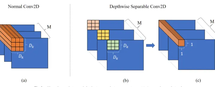
Fig. 2 Normal convolution and depthwise convolution comparison. (a) A normal convolutional operation with kernel sizeDk×Dk; (b) depthwise convolutional operation with the same size as (a);

(c) pointwise convolutional operation with kernel size 1×1. Dk is the kernel size. M represents the number of input feature maps.

the performance of inputs into the dataset. Data standardization/normalization makes the dataset space more compact and consistent with the range of output values and enables the gradient descent distance between each step is shorter. In this research, considering the process of tongue diagnosis, the flowing data augmentation strategies have been applied:

• Rotation with angle 10^◦

• Horizontal Flip

Since Batch Normalization (BN)[16]is applied in each convolutional block of our designed network, we only use data normalization in the preprocessing part. Directly apply the following method to normalize both input images and labels into the range [−1,1]:

p_[−1,_1]= p

255−1 (1)

To get predictions in [0, 1], process the predicted mask with Eq. (2):

p_[0,_1]=2p[−1,1]−1, (2) wherepmeans the intensity of pixel value, subscript means the value range.

3.2 Batch Normalization and ReLU

Batch normalization generally followed by ReLU[17]nonlinear activation function can speed up the training process.

Our training dataset contains different contrast RGB image.

Hence, it is necessary to use batch normalization to reduce the covariate-shift[16] between images in one batch data.

Meanwhile, batch normalization can prevent vanishing gradients and exploding gradients behaviours.

3.3 Depthwise Separable Convolution

As shown in Fig. 2, depthwise separable convolution contains two steps. The first step is depthwise convolutional step applying different kernels independently on each feature map which works as a filtering process. The second step uses pointwise convolutions with kernel 1×1 to sum- marize previous convolutional results into the final feature map. Considering the number of multiplication operations in two kinds of convolutional operations, define the kernel size and the number of input feature maps as shown in the figure. The number of multiplication operations in the normal convolutional operation can be calculated as below:

N_{nor m}=N M D_k², (3)

where D_k is the kernel size. M represents the number of input feature maps. For depthwise separable convolution:

N_dep.sep.=M(D_k²+N), (4)

whereNmeans the number of kernels in both cases. N_{nor m} and N_dep.sep. represent the number of multiplication operations for normal convolution and depthwise separable convolution, respectively. According to Eq. (3) and Eq. (4), the multiplication calculation is reduced *

, 1 N + 1

D²

k

+ -

times by replacing normal convolution with depthwise spreadable convolution. Some related works [18]–[20] have proved that the depthwise spreadable convolutions does not degrade performance with the multiplication reduction. On the contrary, sometimes it can improve the convergence performance. This is possibly due to the independently multiple kernels for each feature map which can gains the chance to avoid the local minima.

(4)

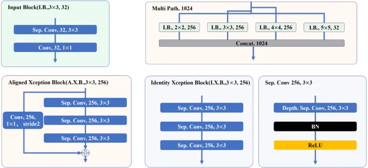
Fig. 3 The block components in the designed architectures. The above convolutional operation without stride specification means operation with stride 1. “Sep. Conv” means depthwise separable convolutional operation as mentioned in Sect. 3.3. “BN” refers to batch normalization. “ReLU” means ReLU nonlinear activation function. “I.B., 2×2, 256” means input block structure consists of 256 kernels with kernel size 2×2.

3.4 Modified Aligned Xception Block

The modified Aligned Xception Block (AXB) is proposed by DeepLab v3+[12]. [12],[18],[20]have exhibited good performance of Xception block in classification and segmentation tasks. Hence, the basic block in our designed architecture preserved the same structural unit. The modified aligned Xception block has the similar structure as ResNet convolutional block [15]which contains shortcut from input added directly with the output features of the block as shown in Fig. 3. The shortcut path is a normal convolutional operation with stride of 2. It is necessary to state that all the 1×1 convolution operations in our designed architecture are standard 2D convolution without BN and ReLU. Each depthwise separatable convolutional operation in one block as mentioned in Sect. 3.2 all followed by BN and nonlinear activation ReLU.

3.5 Architecture

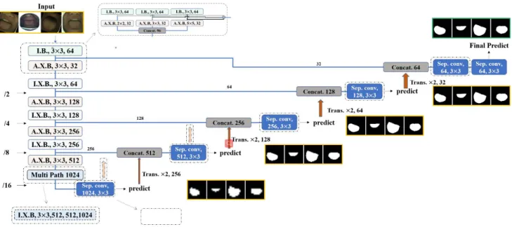
In this research, we have several designs according to our pyramid predictive design(see Sect. 3.5.2) philosophy. By trade-off of training efficiency, convergence speed, and inference time consumption, we choose the model as exhibited in Fig. 4 to be our final proposal. It follows the typical encoder-decoder framework and mainly contains four kinds of blocks (see Fig. 3). Compared to DeepLab v3+, our network is much shallower which will be more suitable for small dataset and inference faster usually. At the end of the encoder, we use multipath block which consists of four 256-IBs(Multi Path block in Fig. 3) with multi-scale kernel

sizes.

3.5.1 Encoder

The number of kernels for each layer is the same inside all kinds of blocks. The number of filters is doubled as the dimension halved.

Input block (IB) is only used for the starting point and end point (the last block) of the encoder. Each IB contains only one 3×3 depthwise separable convolutional layer attached with a 1×1 standard convolutional layer. From the beginning of the PPAN, the 1×1 standard convolution in IB plays the role of the color palette and feature integration.

In our training dataset, the RGB images contain multiple hues. We expect that the network can adjust hues from the beginning to make BN easier to norm with smaller variance inside one batch data. It is also an implicit input augmentation. The smaller number of convolutional features in the beginning is also benefit for GPU memory consumption and inference speed. Since the raw input image has the largest resolution and the highest information accuracy, we want to keep the raw information for the later concatenation in order to get the more accurate final segmentation result in the end.

In the middle dimension stages, each contains one AXB and one Identity Xception Block (IXB). The exact setting for the number of kernels for each layer can be found in Fig. 4 according to the definition in Fig. 3. IXB does not contain shortcut compared to AXB. The shortcut in AXB can smooth the parameter tuning[15],[18]. AXB has been introduced in Sect. 3.4.

At the end of the encoder, we attached the Multi-Path Block (MPB) which consists of four IBs with four different

(5)

Fig. 4 The designed baseline architecture of proposed segmentation network. “I.X.B., 64” indicate identity block with 64 kernels for all components inside the block as showed in Fig. 3. “A.X.B., 128”

means aligned Xception block with 128 kernels for all components inside the block. It is the same for other numbers with prefixes of “A.X.B.” and “I.X.B.”. “Multi Path 1024” is the exactly same as shown in Fig. 3. “I.X.B, 3×3, 512,512,1024” means identity Xception block with the filter number respectively 512, 512, 1024, which is not the same as definition in Fig. 3. Dotted line in the figure means the experiment attempts in this research (more details can be found in Sect. 4).

kernel sizes (2×2, 3×3, 4×4, 5×5). With the same purpose as PPM and ASPP, MPB helps the network to capture global context information of the entire image under the smaller dimension feature maps. The dimension of input for our network is 256 resulting in the last dimension in MPB to be 16 (1/16 of input dimension). With 5×5 kernels size, it can compute around one-third of the input image. Considering either ASPP or PPM will introduce pixel errors directly due to the discrete kernels and pooling strategy, the compact kernels should work better for the segmentation task.

3.5.2 Pyramid Predictive Attention in Decoder

In the decoder path, it works similarly as U-Net containing both skip-connection (concatenation) and transposed convolution. The key differences are that our tranposed operations are applied on the predictions not on the feature maps and we have multiple segmentation predictions on each dimension stage which are synchronously optimized with the defined cost function(see Sect. 3.6).

Before transposing the lower dimension to a higher dimension in each dimension stage, one group 3×3 of depthwise separable convolutions and one predictive convolutional layer are applied (see Fig. 4). Each of 3×3 convolutions is for integrating the coarse feature maps with lower dimension to make the feature maps able to use for each prediction directly. The convolutions before prediction in lower dimension can also reduce the burden of higher dimension integrating task. In the end, each stage 3×3 convolutions will make the final stage (raw dimension) 3×3 convolutions before the final prediction easier to process. The nonlinear

activation used for prediction is tanh [15] function which will map the input value to(−1,1)range. Tanh compared to sigmoid having larger derivative making the training process more efficient. Since we have multiple prediction operations, tanh is a better choice than sigmoid.

In our designed PPAN, transposed convolution is no longer applied on feature maps but the prediction with lower dimension. By directly predictions transposed, the memory cost in the network will be reduced. Furthermore, predictions from each dimension stage will be optimized by the same optimizer which is equally to pyramid optimization of the multi-scale predictions. The backward propagation will also be more natural with pyramid prediction strategy. It is not easy to tell the significant depth of the network for image segmentation task. However, the truth is that most accurate pixel information is the raw input image itself. The deeper of the network, the pixel information more deviate from the ground truth. Therefore, using our designed pyramid prediction and transposed from prediction will maximize the use of near-layer (the layer closer to the raw input, the more accurate pixel information, maximizing the utilizing of encoder feature maps) information without paying too much efforts on the deeper redundancy. At the same time, predictions from each dimension stage can make the network concen- trate on the local attention of each feature map from the encoder efficiently improved the feature representation (see Fig. 1, tongue boundary is more obvious in the mean feature maps) by concatenating the encoder feature maps with tranposed predictions. On the whole, the pyramid optimization combined with the local attention model will greatly optimize the training process, which is convenient for the model

(6)

The optimization algorithm used in this research is Adaptive Moment Estimation (Adam)[25], which is the combination of RMSProp[26]and momentum[27]. From[25], they em- pirically demonstrate that Adam generally works better than other stochastic optimization methods. Hence, we choose Adam to be our optimization choice in this research. The details of the parameters settings of this research implementation can be found in Sect. 4.

3.6.1 Cost Function

The final cost function formulated in this research is made of 3 kinds of weighted cost functions as following:

J_{tot al}(W,b) =αJ_Dice(W,b)+βJ_L₁(W,b)

+γJ_{SC E}(W,b), (5) where

J_Dice(W,b) = 1−Dice_coe, (6) and

Dice_coe = 2

n

X

i=1

yˆ_iy_i Xn

i=1

yˆ_iyˆ_i+ Xn i=1

y_iy_i

, (7)

Each pixel prediction ˆy_iand each pixel label y_iare in a pair of predicted maps at the pixel positioni. The numerator in Eq. (7) expresses the two times of intersection between predicted map and label map. When the predicted map is the same as label map, Eq. (7) is equal to 1. This definition is given by TensorLayer[28]. The shape of each map is [2,256,256,1]. Hence,n=2×256×256×1=131072 in Eq. (7). TheL₁-norm cost function for prediction and label is:

J_L₁(W,b) = 1 n

n

X

i=1

||yˆ_i−y_i||₁ (8) From the research work[7], it demonstrates thatL1-norm en- courages less blurring compared toL2-norm. The last term in Eq. (5) is the sigmoid-cross-entropy (SCE) cost function

to match the label distribution. Meanwhile, L1-norm will ensure the value closed to the label value based on distri- butions matched. The final evaluation will use Intersection over Union (IoU) metric to judge the segmentation performance, IoU and dice coefficient essentially are the same.

Hence, adding dice cost into the minimization will straight- forward improve the final performance. In some researches, dice coefficient is also used as an evaluation metric for medical image segmentation. All the cost functions mentioned above are synchronously optimized for different dimension predictions (As mentioned in Sect. 3.5.2).

3.6.2 Evaluation Metric

Intersection over Union (IoU) is defined as its name, sometimes called Jaccard Index[29]:

IoU= |A∩B|

|A∪B|. (11)

This metric is always used to evaluate the pixel-level segmentation quality and bounding box precision[30]–[32]. It is more sensitive to the positive predictions compared to ROC [33]metric for binary classification (binary segmentation can be interpreted as binary classification). The dice coefficient can also be converted to IoU by the following equation:

IoU= Dice

2−Dice. (12)

In the next section, the experiment in this research will be introduced.

4. Experiment

4.1 Dataset Description

The acquired tongue RGB images were shot with Tongue Image Analyzing System (TIAS[34]). Due to the upgrade of system equipment and different shooting time, images contain different hues and resolutions.

In order to simplify the experimental procedure, the images were split into the a training set, validation set and test set concerning around rate 3:1:1. The total number of

(7)

Table 1 Performance with different design candidates compared to U-Net.

Model Name Top Multi-Path Bottom Multi-Path Transpose from

Conv.

Before Pred.s

# Top 64

Conv.s M.M.IoU A.M.IoU M.Infer.

Time

M.VIoU Slope (e⁻⁵)

Variable Size (≈Bytes) U-Net +

Dice / / / / / 0.932161 0.929102 0.079946 / 124181764B

Design v1 [2x2, 3x3, 5x5] [2x2, 3x3, 4x4, 5x5] all stage

pred.s X 2 0.931306 0.927888 0.103371 5.04 14527448B

(−88.30%) Design v2 [3x3, 3x3, 3x3] [2x2, 3x3, 4x4, 5x5] all stage

pred.s X 2 0.924552 0.921599 0.101824 6.04 14521816B

(−88.31%) Design v3 [2x2, 3x3, 5x5] [2x2, 3x3, 4x4, 5x5] F: /16,/8;

P: /4, /2 X 2 0.928789 0.927208 0.105204 6.57 35474392B

(−71.43%) Design v4 IB+ AXB [2x2, 3x3, 4x4, 5x5] all stage

pred.s X 2 0.931254 0.929375 0.081483 7.81 14405632B

(−88.40%) Design v5 IB+ AXB [2x2, 3x3, 3x3, 5x5] all stage

pred.s X 2 0.928971 0.926642 0.084232 6.05 14391296B

(−88.41%)

Design v6 IB+ AXB IXB all stage

pred.s X 2 0.929731 0.928288 0.080295 7.40 15407104B

(−87.59%)

Design v7 [2x2, 3x3, 5x5] IXB all stage

pred.s X 2 0.934008 0.931902 0.106013 4.49 15528920B

(−87.50%)

pred.s 7 2 0.929518 0.926393 0.075178 4.17 9744384B

(−92.17%)

pred.s 7 1 0.925298 0.922802 0.071964 4.44 9724928B

(−92.15%)

images in the entire dataset is 443. Among those, the training dataset has 265 images. The size of validation dataset equals the size of the testing dataset with 89 images.

All the images in the entire dataset were resized to 256×256 and normalized into [−1,1] (see Eq. (1)). After normalization, the dataset is processed with data augmentation strategies as described in Sect. 3.1, shuffled and repeated with 50 epochs. Batch size is 2. Therefore there is 1060 batches in each epoch. In total, 53000 batches will be used for training our network. Due to tanh was applied for predictions, the output is also in the range [−1,1] (associated with bias in the convolutional operation). To make predictions in the range [0,1], simply apply Eq. (2).

4.2 Hyper-Parameters Settings for Training Process As described in Sect. 3.6, Adam optimizer is applied. β₁ (TensorFlow v.1.90[35]) was set to 0.5. This is quite smaller value compared to the commonly used setting (0.9[35]). We expect the exponentially weighted averages of gradients can be closer to real gradients in the case of that the model can be optimized more finely for the pixel-level segmentation task.

Other parameters of Adam were directly set to default in TensorFlow. The learning rate was set to 0.0002. The three weighted factorsα, β,γare set to 2, 1, 1 corresponding to dice cost,L1-norm cost and SCE cost (in Eq. (5)).

4.3 Design Cases

In this research, several cases were designed by considering the following aspects (see Fig. 4 and Table 1):

• Multi-path block at the top of the encoder

• Multi-path block at the bottom of the encoder

• From which stage to transpose

• Whether to use 3×3 convolutions between the down- sampling features and prediction for each dimension stage

• The number of 64-convolutional operations

The effect of the dice cost function is also evaluated by comparing the performance with U-Net, Res50-FPN and DeepLab v3+(Xception 65).

5. Results and Discussion

The evaluated results are as shown in Table 1 and Table 2.

Table 1 is about the exploration for the model design with considerations listed in the table. All the models trained in Table 1 as described in previous sections optimized with dice cost function. From Table 2, it shows that the average mean IoU is improved by introducing the dice cost into the total cost. IoU results are evaluated under the thresholds range from 0.05 to 0.95 with 10 samples. In both tables,

“M.M.IoU” means the Maximum value of mean IoUs across the whole threshold span for all batches. “A.M.IoU” tells the average value accordingly. The items listed in Table 1 has been explained at Sect. 4.3. The list (e.g. [2×2, 3×3, 5×5]) in the columns related to “Multi-path” means the kernel sizes.

“IB+AXB” means top multi-path block of designed network (Fig. 4) is replaced by IB and followed by AXB (defined in Sect. 3.5.1). Notation “IXB” in bottom multi-path block means replacing bottom multi-path block with single IXB as explained in the caption of Fig. 4. “M.VIoU Slope” is cal-

(8)

“VIoU Slope” is the average slope value for each increment between two recorded steps. “M. VIoU Slope” is the mean slope value for the whole training process. The larger of

“M.VIoU Slope,” the stronger of validated IoU increased.

For the “transposed from” aspect, only two cases for the consideration of applying transposed. One is applying transposed convolution on each stage prediction as proposed idea in this paper (Pyramid Predictive Attention, denoted as “all stage pred.s” in Table 1 and “predict” in Fig. 4). In another case, transpose feature maps before prediction in the lower dimension stage (1/16, 1/8) and predictions are transposed for the higher dimension stage (1/4, 1/2), which is denoted as “F: /16, /8; P: /4, /2”. We gave the hypothesis that lower dimension feature maps might contains richer information than the pure single prediction, which could benefit from the final segmentation. Nevertheless, by comparing Design v3 with Design v1, this hypothesis is not true. With more lower dimension feature maps transposed, in addition to enhanc- ing the convergence of validated IoU in the training process, other aspects all have had a negative impact.

Another unexpected result is the performance degrade quite a lot 0.007 (compared to other degrades) percentage points when changing the top multi-path kernels from di- verse kernel size (Design v1) to all 3×3 kernels keeping the multi-path property (Design v3). Design v4 is the same model as shown in Fig. 4. Analyzing from all the considerations, Design v4 has the performances with small variable size; high average mean IoU, high validation IoU convergence ability and relatively short inference time (denoted as

“M.Infer.Time”). Therefore, we propose the Design v4 to be our final design. There is another high-performance model as shown in Design v7. Both maximum mean IoU and average mean IoU are the highest from all the trained models’

performance. However, the inference time and variables size are increased due to the large dimension multi-path block at the top of the encoder. Comparing Design v1/v2/v3/v7 with other designs, it proves that put multi-path at the large dimension stage will increase the inference time. Without considering the variable size and inference time, Design v7 is also a good choice for tongue segmentation. Another important finding is that the top-64 convolutions have an essential role for validation IoU convergence and the final average mean IoU performance by comparing Design v9 with Design v8

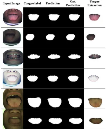
Fig. 5 The segmentation results of Design v4 on the test dataset. “Predic- tion” means the results are directly generated from the network. “Opt. Pre- diction” means “Optimal Prediction” in which the results are produced by thresholding the “Prediction” results concerning the largest IoU value.

“Tongue Extraction” results are the multiplication results of “Input Image”

and “Opt. Prediction”.

and Design v6.

All of the designs (in Table 1) work for current training dataset to segment tongue images, they all have mean average IoU performance more than 0.9 which is significant for pixel level segmentation task. As known, the deep learning algorithm is highly dependent on the dataset. Since we are using our own dataset, it is hard to compare our performance to others’ tongue segmentation performance. Without the same dataset, the comparison does not have too much sense in the deep learning world. Our main purpose in this research work is to reduce the memory consumption for the networks and keep the performance. We have picked 3 most popular (top performance on other dataset) encoder-decoder segmentation networks and evaluated in the Table 2. Compared to those popular networks, our designed network has similar or better segmentation performance. More importantly, our designs saved memory around 71% to 92% compared to U- Net (In most of segmentation networks, U-Net is the most shallow and small network), which will be a significant ad- vantage when deploying the segmentation network into the limited storage terminals. Our pyramid predictive attention design can contribute at least 15% memory saving compared to traditional up-sampling decoder without any performance degradation (compare Design v1 and Design v3).

Figure 5 shows the visualized segmentation results of Design v4 on the test dataset. As we can see, the designed

(9)

network can extract tongue from images with different hues, different posture, and different resolutions. It is robust to the contrast shift.

6. Conclusion

In this research, our team evaluated the popular segmentation models for the segmentation of tongue diagnosis images.

Although our dataset is quite challenge for the training (all the tongue images are acquired by different cameras with different resolutions and hues at the different time), we still get the IoU performance more than 0.9. In the proposed designs, the depthwise separable convolutions are applied, which are much more efficiency convolutional operations compared to the standard 2D convolutions.

We designed pyramid predictive attention functionality in the decoder by concatenating the feature maps with the tranposed predictions from the lower dimension. Multi-scale predictions are generated with multi-synchronous optimiza- tions. This provides a kind-of self attention to smooth in the upsampling path. By pure transposing the prediction from lower dimension to a larger dimension, the computation efficiency is future improved without the performance degrade. This kind of design can inspire other researchers a new thinking for attention based or region based segmentation task. We successfully achieved to reduce memory consumption around 80% without performance degrade. The pyramid predictive attention design contributes more than 15% memory saving. This provides a basis for the de- velopment of the future mobile diagnostic system and the tongue-based sublingual vein segmentation.

From our designed and tested results, multi-path design in the high dimension stage increase the inference time;

transposed operations applied on predictions of each dimension stage does not degrade the performance; convolutions at large dimension stage (raw dimension of input) play a vital role in order to improve the segmentation results.

In the future segmentation project, especially tongue related image segmentation, we will consider adding more images with individual cases to improve the robustness to tongue images shot in an unexpected situation. From the design considerations, we would investigate the global attention (global pooling multiplication) effect for the image segmentation task and Binary Neural Network (BNN[36]) in the future work. Although, the depthwise separable convolutional operation is efficient in multiplication calculation, the inference speed does not significantly improved. Therefore, BNN could possessively bring a leap in speed of interference, since it change full precision weights to binary weights.

References

[1] X. Li, H. Chen, X. Qi, Q. Dou, C.W. Fu, and P.A. Heng, “Hdenseunet:

Hybrid densely connected unet for liver and liver tumor segmentation from CT volumes,” arXiv preprint arXiv:1709.07330, 2017.

[2] A. Krizhevsky, I. Sutskever, and G.E. Hinton, “Imagenet classification with deep convolutional neural networks,” Advances in Neural Information Processing Systems, pp.1097–1105, 2012.

[3] J. Long, E. Shelhamer, and T. Darrell, “Fully convolutional networks for semantic segmentation,” Proc. IEEE conference on computer vision and pattern recognition, pp.3431–3440, 2015.

[4] J. Nagi, F. Ducatelle, G.A. Di Caro, D. Ciresan, U. Meier, A. Giusti, F.

Nagi, J. Schmidhuber, and L.M. Gambardella, “Max-pooling convolutional neural networks for vision-based hand gesture recognition,”

Signal and Image Processing Applications (ICSIPA), 2011, IEEE International Conference on, pp.342–347, IEEE, 2011.

[5] O. Ronneberger, P. Fischer, and T. Brox, “U-Net: Convolutional networks for biomedical image segmentation,” International Conference on Medical image computing and computer-assisted intervention, pp.234–241, Springer, 2011.

[6] G. Huang, Z. Liu, L. Van Der Maaten, and K.Q. Weinberger,

“Densely connected convolutional networks,” CVPR, p.3, 2017.

[7] P. Isola, J.Y. Zhu, T. Zhou, and A.A. Efros, “Image-to-image translation with conditional adversarial networks,” arXiv preprint arXiv:1611.07004v2, 2017.

[8] L.C. Chen, G. Papandreou, I. Kokkinos, K. Murphy, and A.L. Yuille,

“Semantic image segmentation with deep convolutional nets and fully connected CRFs,” arXiv preprint arXiv:1412.7062, 2014.

[9] H. Zhao, J. Shi, X. Qi, X. Wang, and J. Jia, “Pyramid scene parsing network,” IEEE Conf. on Computer Vision and Pattern Recognition (CVPR), pp.2881–2890, 2017.

[10] L.C. Chen, G. Papandreou, I. Kokkinos, K. Murphy, and A.L. Yuille,

“Deeplab: Semantic image segmentation with deep convolutional nets, atrous convolution, and fully connected CRFs,” IEEE Trans.

Pattern Anal. Mach. Intell., vol.40, no.4, pp.834–848, 2018.

[11] L.C. Chen, G. Papandreou, F. Schroff, and H. Adam, “Rethinking atrous convolution for semantic image segmentation,” arXiv preprint arXiv:1706.05587, 2017.

[12] L.C. Chen, G. Papandreou, F. Schroff, and H. Adam, “Encoder- decoder with atrous separable convolution for semantic image segmentation,” arXiv preprint arXiv:1802.02611, 2018.

[13] K. He, G. Gkioxari, P. Dollár, and R. Girshick, “Mask R-CNN,”

Computer Vision (ICCV), 2017 IEEE International Conference on, pp.2980–2988, IEEE, 2017.

[14] T.Y. Lin, P. Dollár, R.B. Girshick, K. He, B. Hariharan, and S.J.

Belongie, “Feature pyramid networks for object detection,” CVPR, p.4, 2017.

[15] K. He, X. Zhang, S. Ren, and J. Sun, “Deep residual learning for image recognition,” Proc. IEEE conference on computer vision and pattern recognition (CVPR), pp.770–778, 2016.

[16] L. Chen, H. Fei, Y. Xiao, J. He, and H. Li, “Why batch normalization works? a buckling perspective,” Information and Automation (ICIA), 2017 IEEE International Conference on, pp.1184–1189, IEEE, 2017.

[17] S. Woo and C.L. Lee, “Decision boundary formation of deep convolution networks with relu,” 2018 IEEE 16th Intl Conf on Dependable, Autonomic and Secure Computing, 16th Intl Conf on Pervasive Intel- ligence and Computing, 4th Intl Conf on Big Data Intelligence and Computing and Cyber Science and Technology Congress (DASC/

PiCom/DataCom/CyberSciTech), pp.885–888, IEEE, 2018.

[18] F. Chollet, “Xception: Deep learning with depthwise separable convolutions,” arXiv preprint arXiv:1610.02357, 2017.

[19] A.G. Howard, M. Zhu, B. Chen, D. Kalenichenko, W. Wang, T.

Weyand, M. Andreetto, and H. Adam, “MobileNets: Efficient convolutional neural networks for mobile vision applications,” arXiv preprint arXiv:1704.04861, 2017.

[20] L. Kaiser, A.N. Gomez, N. Shazeer, A. Vaswani, N. Parmar, L. Jones, and J. Uszkoreit, “One model to learn them all,” arXiv preprint arXiv:1706.05137, 2017.

[21] R. Zaheer and H. Shaziya, “GPU-based empirical evaluation of activation functions in convolutional neural networks,” 2018 2nd In- ternational Conference on Inventive Systems and Control (ICISC), pp.769–773, Jan 2018.

[22] V. Zyuzin, P. Sergey, A. Mukhtarov, T. Chumarnaya, O. Solovyova, A. Bobkova, and V. Myasnikov, “Identification of the left ventri- cle endocardial border on two-dimensional ultrasound images using

(10)

[28] L.M.F.L.A.O.S.Y.Y.G. H. Dong, and A. Supratak, “Tensor- layer: A versatile library for efficient deep learning develop- ment,” URL: https://tensorlayer.readthedocs.io/en/stable/modules/

cost.html?highlight=dice/, 2018 [Online; accessed 17-Dec.-2018].

[29] P. Jaccard, “Étude comparative de la distribution florale dans une portion des alpes et des jura,” Bull. Soc. Vaudoise Sci. Nat., vol.37, 2018.

[30] F. Meng, H. Li, Q. Wu, K.N. Ngan, and J. Cai, “Seeds-based part segmentation by seeds propagation and region convexity decompo- sition,” IEEE Trans. Multimedia, vol.20, no.2, pp.310–322, 2018.

[31] V. Iglovikov and A. Shvets, “Ternausnet: U-Net with VGG11 encoder pre-trained on ImageNet for image segmentation,” arXiv preprint arXiv:1801.05746, 2018.

[32] A. Shvets, V. Iglovikov, A. Rakhlin, and A.A. Kalinin, “Angiodys- plasia detection and localization using deep convolutional neural networks,” arXiv preprint arXiv:1804.08024, 2018.

[33] T. Fawcett, “An introduction to ROC analysis,” Pattern Recogn. Lett., vol.27, no.8, pp.861–874, 2006.

[34] N. Toshiya, “Tongue imaging and analysis system-TIAS,” URL:

http://nlab.tms.chiba-u.jp/topics.html, 2018 [Online; accessed 17- Dec.-2018].

[35] G. Brain, “Adamoptimizer,” URL: https://www.tensorflow.org/

versions/r1.9/api_docs/python/tf/train/AdamOptimizer, 2018 [On- line; accessed 17-Dec.-2018].

[36] J. Bethge, M. Bornstein, A. Loy, H. Yang, and C. Meinel, “Training competitive binary neural networks from scratch,” arXiv preprint arXiv:1812.01965, 2018.

Tingxiao Yang received B.E. and M.D. degrees from University of Gävle, Electronics and Telecommunications in 2012 and 2013 respectively. He became a Ph.D. graduate student, Department of Medical Engineering, Graduate School of Science and Technology, Chiba Uni- versity, Japan in 2018. His current research interests including image processing, computer vision and computer graphics, especially in deep learning.

in 2014. He received Ph.D. degree from Chiba University, Chiba, Japan in 2018. He is currently a Part-time Lecturer, Department of Japanese- Oriental (Kampo) Medicine, Graduate School of Medicine, Chiba University, Japan. He is specialized in Acupuncture/Moxibustion and Japanese Traditional (Kampo) medicine.

Takao Namiki received B.E. and M.D. degrees from Chiba University, School of Medicine in 1985 and 1993 respectively. He became an Associate Professor, Department of Japanese- Oriental (Kampo) Medicine, Graduate School of Medicine, Chiba University, Japan in 2010.

He is currently a Director of Department of Japanese-Oriental (Kampo) Medicine, Chiba University Hospital, Chiba University since 2011. He is specialized in internal medicine, cardiology and Japanese Traditional (Kampo) medicine.

Toshiya Nakaguchi received B.E., M.E., and Ph.D. degrees from Sophia University, To- kyo, Japan in 1998, 2000, and 2003, respectively.

He was a research fellow supported by Japan So- ciety for the Promotion of Science from 2001 to 2003. He moved to the Department of In- formation and Image Sciences, Chiba University in 2003, as an assistant professor. He moved to the Department of Medical System Engineering, Chiba University in 2010 as an associate professor. He moved to Center for Frontier Medical Engineering, Chiba University in 2013, as an associate professor. He is currently a professor in Center for Frontier Medical Engineering, Chiba University since 2016. His research interests include medical engineering, color image processing, computer vision and computer graphics.