LETTER
A General Perfect Cyclic Interference Alignment by Propagation Delay for Arbitrary X Channels with Two Receivers
Conggai LI†, Feng LIU†a), Shuchao JIANG††,Nonmembers,andYanli XU†,Member
SUMMARY Interference alignment (IA) in temporal domain is impor- tant in the case of single-antenna vehicle communications. In this paper, perfect cyclic IA based on propagation delay is extended to theK×2 X channels with two receivers and arbitrary transmittersK ≥ 2, which achieves the maximal multiplexing gain by obtaining the theoretical de- gree of freedom of 2K/(K+1). We deduce the alignment and separability conditions, and propose a general scheme which is flexible in setting the index of time-slot for IA at the receiver side. Furthermore, the feasibility of the proposed scheme in the two-/three- Euclidean space is analyzed and demonstrated.
key words: K×2X channel, propagation delay, cyclic interference align- ment, degree of freedom, feasibility
1. Introduction
Interference alignment (IA) technique[1]has become one of the most promising approaches, which overlaps the inter- ference in the same signal space to increase the multiplexing gain. It has been widely applied in many models such as in- terference channels (IC)[1]and X channels (XC) [2] and helps achieve the maximal multiplexing gain indicated by the concept of degree of freedom (DoF).
Basically IA can be implemented in the spatial domain.
There are many works such as[3],[4] on applying IA in multiple-antenna systems such as the 3GPP long-term evo- lution. On the other hand, if each node is equipped with only single antenna, implementation of IA in temporal do- main provides an important alternative at the cost of rela- tively large propagation delay (PD).
Seeking IA in the temporal domain attracted some at- tentions such as[5]–[8], which utilizes the PD difference among links and is suitable for the scenario of long PD communications including underwater acoustic networks (UANs). In[9], perfect PD-based cyclic IA was first studied for the 2×2 XC andK-user IC to achieve the DoF of 4/3 andK/2, respectively. Recently, we investigate the perfect IA based on proper PD structure forK×2 XC in[10], while further node placement analysis is given in[11]. Moreover, for the three-user X channel, since perfect IA is impossible [12], we propose a feasible scheme with one extra time slot to achieve the maximum DoF by allowing one more mes-
Manuscript received February 21, 2019.
Manuscript revised July 6, 2019.
†The authors are with the College of Information Engineering, Shanghai Maritime University, Shanghai, China.
††The author is with the School of Information Science and Technology, Fudan University, Shanghai, China.
a) E-mail: [email protected] DOI: 10.1587/transfun.E102.A.1580
sage based on the cyclic IA approach[13].
However, [10]provided only one feasible PD pattern with perfect IA forK×2 XC and pointed out that theK=2 case is a special case of the cyclic IA[9]. It is natural to ask that if the perfect PD-based cyclic IA can be extended to the generalK×2 XC, which leads us to this article.
In this work, we successfully extend the cyclic IA tech- nique for XC from the basic 2×2 case to the generalK×2 following the framework of the cyclic PD-based model[9].
The alignment and separability conditions of perfect cyclic IA are deduced, which achieves the DoF of 2K/(K+1).
Compared to[10], a general scheme withK+1 PD patterns is provided, where the index of time-slot for perfect cyclic IA at the receiver side can be arbitrarily determined by a system parameterK1. Furthermore, the feasibility condition is deduced in the Euclidean space.
2. System Model
The K ×2 XC has K (K ≥ 2) source nodes Sk,∀k ∈ {1,2,· · ·,K} and two destination nodes Dj,∀j ∈ {1,2}, where each node has single antenna. The message fromSk toDjis denoted byWk,j. Totally, there are M =2Kinde- pendent and different messages. Perfect synchronization is assumed among all communication nodes.
Equally sized time-slots are partitioned and normalized for the channel, while each message occupies one time-slot.
The transmission is divided into n ∈ Nconsecutive time- slots as a cycle, i.e., the cyclic delays are unrolled over time.
The PD between any Sk andDj are assumed to be static and non-negative integer multiples of one time-slot. The channel access is stationary over a period ofnconsecutive time-slots. Within the stationary period, delayed messages are cyclically right-shifted. Afterntime-slots new messages are transmitted and the procedure repeats again.
Similar to [9], cyclic right-shift by polynomials in x modulo xn − 1 is used for modeling. Single time- slot in the period of n time-slots is addressed by offsets x0,x1,· · ·,xn−1, from 0 (no offset) ton−1 (maximal off- set). Here zero-offset indicates a reference PD. The in- teger PD between Sk to Dj is denoted by τk,j ∈ D = nxi|i=0,1,· · ·,n−1o
. We define the following K×2 PD matrix Dwith elementsdk,j in polynomial form
Copyright c2019 The Institute of Electronics, Information and Communication Engineers
D=
d1,1 d1,2
d2,1 d2,2
... ... dK,1 dK,1
,
xτ1,1 xτ1,2 xτ2,1 xτ2,2 ... ... xτK,1 xτK,1
(1)
and assume it to be known at all nodes before transmission.
For a messageWto be transmitted at offsetxuand de- layed byvtime-slots, the resulting delayed message can be computed by xu+vW mod (xn −1) for a period ofn. For brevity, we denote mod (xn−1) as modXn.
Encoding procedure: The codeword sent from Sk is encoded into the polynomialvk(x) by the encoding function ekcarrying the two messagesWk,1andWk,2:
ek: (Wk,1,Wk,2)→vk(x) (2) where the input polynomial can be expressed as
vk(x)=Wk,1xpk,1+Wk,2xpk,2 modXn (3) with parameter pk,jindicating the index of allocated time- slot for messageWk,j. The input polynomial vector is
u=h
v1(x) v2(x) · · · vK(x)i
(4) Through the above PD-based model, each receiver obtains a polynomial denoted byrj(x),∀j∈ {1,2}. In the vector form,
r=h
r1(x) r2(x)i
≡uD modXn (5)
Decoding procedure: AtDj, the received polynomial rj(x) is decoded to obtain the dedicated messages:
fj:rj(x)→( ˆW1,j,Wˆ2,j,· · ·,WˆK,j) (6) For this PD-based model, its DoF is defined by DoF, M
n =2K
n (7)
Remark: To focus on the core problem of PD-based IA, we assume unit-gain channels and zero noises as well as that in[9]. In fact, different channel gains among all source- destination pairs are also allowed in the system model. In this case, channel estimation and equalization techniques should be applied at each receiver before the above decoding procedure.
3. A General Perfect Cyclic IA Scheme
From the existing result of general XC[2], the maximum achievable DoF ofK×2 XC is 2K/(K+1). In the PD-based model, we haveM =2K different messages to convey and decode over a period ofntime-slots. To achieve the theoret- ical DoF of 2K/(K+1), the minimal number of consecutive time-slots at the decoder side should be equal ton=K+1.
Otherwise, a larger period will decrease the achieved DoF, which makes the scheme suboptimal. In the following con- tent, we only discuss this DoF-optimal configuration based
on perfect cyclic IA over the above PD-based model.
Since each decoder needs Ktime-slots to separate its requiredKmessages, only one time-slot is available for per- fect cyclic IA. In detail, Dj should align its K undesired messagesWk,¯j,∀k∈ {1,2,· · ·,K},¯j, jas interference into one of the totalK+1 time-slots, which brings thealignment conditions:
dk,jxpk,¯j ≡ dl,jxpl,¯j modXK+1
⇔ xτk,j+pk,¯j ≡ xτl,j+pl,¯j modXK+1
⇔ τk,j+pk,¯j ≡ τl,j+pl,¯j modK+1
(8)
with∀k,l∈ {1,2,· · ·,K}and j,¯j∈ {1,2}.
On the other hand, the desiredKmessagesWk,jshould be distinct with each other and occupy all the Ktime-slots except the one for cyclic IA, which introduces thesepara- bility conditionsatDj:
dk,jxpk,j . dl,jxpl,j modXK+1
⇔ xτk,j+pk,j . xτl,j+pl,j modXK+1
⇔ τk,j+pk,j . τl,j+pl,j modK+1
(9) for theKmessages with∀k,l∈ {1,2,· · ·,K}, and
dk,jxpk,j . dl,jxpl,¯j modXK+1
⇔ xτk,j+pk,j . xτl,j+pl,¯j modXK+1
⇔ τk,j+pk,j . τl,j+pl,¯j modK+1
(10) between the message and interference with ∀k , l ∈ {1,2,· · ·,K}and j,¯j∈ {1,2}.
Theorem 1 summarizes our main contribution.
Theorem 1. Perfect cyclic IA achieving the DoF of2K/(K+ 1)for the K×2PD-based X channels exists and a general scheme of[10]is given by the following K×2PD matrix
DK1=
xτ1,1 xτ1,2 xτ2,1 xτ2,2 ... ... xτK1,1 xτK1,2 xτK1+1,1 xτK1+1,2 xτK1+2,1 xτK1+2,2
... ... xτK,1 xτK,2
=
x0 xK2 x1 xK2 ... ... xK1−1 xK2
xK1 x0 xK1 x1 ... ... xK1 xK2−1
(11)
where parameters0≤K1≤K and K2,K−K1are two in- tegers indicating the time-slot index for cyclic IA atD1and D2, respectively, and the following transmitter polynomial
vk(x)=
( Wk,1+xK1−k+1Wk,2 modXK+1, ∀k≤K1
Wk,2+xK−k+1Wk,1 modXK+1, ∀k>K1
(12) Proof. The proof is divided into two parts. Firstly, we show the existence of perfect cyclic IA with a DoF of 2K/K+1.
Then we show the general feature of the proposed scheme in contrast to that in[10].
From (5) withn=K+1, atD1, we have
r1(x) ≡ uDK1(:,1) modXK+1
≡
K1
X
k=1
vk(x)xk−1+
K
X
k=K1+1
vk(x)xK1 modXK+1
≡
K1
X
k=1
(Wk,1+xK1−k+1Wk,2)xk−1 +
K
X
k=K1+1
(Wk,2+xK−k+1Wk,1)xK1 modXK+1
≡
K1
X
k=1
(xk−1Wk,1+xK1Wk,2) +
K
X
k=K1+1
(xK1Wk,2+xK+K1−k+1Wk,1) modXK+1
≡
K1
X
k=1
xk−1Wk,1+
K
X
k=1
xK1Wk,2
+
K
X
k=K1+1
xK+K1−k+1Wk,1 modXK+1 (13) The second term in the last step shows that the alignment conditions (8) are satisfied, since all the interference mes- sages Wk,2,∀k ∈ {1,2,· · ·,K} are aligned into the time- slot K1, i.e., dk,1xpk,2 ≡ dl,1xpl,2 ≡ xK1 modXK+1, with
∀k,l ∈ {1,2,· · ·,K}. The first term indicates that the de- sired messageWk,1is exclusively located in time-slotk−1,
∀k ∈ {1,2,· · ·,K1}, while the third term indicates that the desired messageWk,1 is exclusively located in time-slot K+K1−k+1,∀k∈ {K1+1,K1+2,· · ·,K}. So the sepa- rability conditions (9)–(10) are also satisfied.
Similarly, atD2the received polynomial is r2(x) ≡ uDK1(:,2) modXK+1
≡
K1
X
k=1
vk(x)xK2+
K
X
k=K1+1
vk(x)xk−K1−1 modXK+1
≡
K1
X
k=1
(Wk,1+xK1−k+1Wk,2)xK2 +
K
X
k=K1+1
(Wk,2+xK−k+1Wk,1)xk−K1−1 modXK+1
≡
K1
X
k=1
(xK2Wk,1+xK−k+1Wk,2) +
K
X
k=K1+1
(xk−K1−1Wk,2+xK−K1Wk,1) modXK+1
≡
K1
X
k=1
xK−k+1Wk,2+
K
X
k=1
xK2Wk,1
+
K
X
k=K1+1
xk−K1−1Wk,2 modXK+1 (14) The second term in the last step indicates that the alignment
conditions (8) are satisfied by IA at the time-slot K2. The first term indicates that the desired messageWk,2 is exclu- sively located in time-slot K −k+1,∀k ∈ {1,2,· · ·,K1}, while the third term indicates that the desired messageWk,2
is exclusively located in time-slotk−K1 −1, ∀k ∈ {K1 + 1,K1+2,· · ·,K}. Thus, the separability conditions (9)–(10) are still satisfied.
In summary, 2K different messages are collected over K+1 time-slots, which indicates the DoF of 2K/(K+1) is achieved by the proposed scheme. So perfect cyclic IA ex- ists for the PD-basedK×2 X channels. Moreover, the above deduction also shows that K1andK2indicate the time-slot index of cyclic IA atD1andD2, respectively.
Then what left is the generality proof. For any given K,[10]gives one feasible PD pattern. In contrast, by ad- justing K1 from 0 toK, the proposed scheme can provide K+1 feasible PD patterns. Here we show that the one in [10]is just a special case of this work. This can be verified by setting
( K1 =N, K2=N even K:∀K=2N K1 =N, K2=N−1 odd K:∀K=2N−1
(15) whereN,b(K+1)/2cis the floored integer on (K+1)/2.
For example, ifK=6, we haveN=b7/2c=3 andK=2N, while ifK =5, we haveN =b6/2c= 3 andK =2N−1.
Next we take a closer look. With evenK =2N, the above settingK1 =K2=Ngives the following PD matrix
DN=
x0 xN x1 xN ... ... xN−1 xN
xN x0 xN x1 ... ... xN xN−1
which results in the equivalent PD matrix expression given by Eq. (18) in[10]. Correspondingly, the transmitter poly- nomial (12) becomes
vk(x)=
( Wk,1+xN−k+1Wk,2 modXK+1, ∀k≤N Wk,2+xK−k+1Wk,1 modXK+1, ∀k>N which shows the same scheduling message with Eq. (19) in [10]. With odd K = 2N−1, the above setting K1 = N, K2=N−1 gives the following PD matrix
DN=
x0 xN−1 x1 xN−1 ... ... xN−1 xN−1
xN x0 xN x1 ... ... xN xN−2
which results in the equivalent PD matrix expression given by Eq. (21) in[10]. The corresponding transmitter polyno- mial (12) is
vk(x)=
( Wk,1+xN−k+1Wk,2 modXK+1, ∀k≤N Wk,2+xK−k+1Wk,1 modXK+1, ∀k>N which shows the same scheduling message with Eq. (22) in [10]. Therefore, we have proven that the scheme in[10]just a special case of this paper. In other words, the proposed scheme is a generalization of that in[10]. This completes
the proof.
More discussions are provided below for better under- standing of the features of this general scheme.
The PD matrix (11) can be divided into two parts. The upper part includes the first K1 rows, which has the same PDxK2toD2and increasing PDx0toxK1−1fromS1toSK1. The lower part includes the lastK2rows, which has the same PDxK1 toD1and increasing PDx0toxK2−1fromSK1+1 to SK. The proportion of the upper part is determined byK1. By adjustingK1from 0 toK, the PD matrix has totalK+1 patterns. Specially, ifK1 =0 or equivalentlyK2 =K, the upper part will be an empty matrix without dimension since K1−1=−1. In this case, the PD matrix D0will only have the lower part as shown on the left of (16). On the other hand, ifK1 =Kor equivalentlyK2 =0, the lower part will be an empty matrix without dimension sinceK2−1 =−1.
In this case, the PD matrixDKwill only have the upper part as shown on the right of (16). Thus we have
D0=
x0 x0 x0 x1 ... ... x0 xK−1
, DK=
x0 x0 x1 x0 ... ... xK−1 x0
(16)
forK1=0 andK2 =0, respectively. Accordingly, the input polynomial is
vk(x)=(
Wk,2+xK−k+1Wk,1, K1=0
Wk,1+xK−k+1Wk,2, K2=0 (17) And the received polynomials are
"
r1(x) r2(x)
#
≡
"PK
k=1x0Wk,2+PK
k=1xK−k+1Wk,1
PK
k=1xKWk,1+PK
k=1xk−1Wk,2
#
modXK+1 forK1=0, and
"
r1(x) r2(x)
#
≡
" PK
k=1xk−1Wk,1+PK
k=1xKWk,2 PK
k=1xK−k+1Wk,2+PK
k=1x0Wk,1
#
modXK+1 for K2 = 0, respectively. We can see that the above PD matrices, input and received polynomials withK2 = 0 are equal to that with K1 = 0 if we exchange the role of D1 andD2. So the above cyclic IA scheme exhibits a kind of symmetric property between K1 andK2, i.e., a symmetry within the range ofK1from 0 toK.
On the encoder side, we have some observations from
(12). Whenk≤K1, messageWk,1always occupies the first time slot with index 0, while the other oneWk,2is allocated in the time slot K1−k+1. For example, W1,2 uses time slot K1, andWK1,2 uses time slot 1. Whenk > K1, mes- sageWk,2 always occupies the time slot 0, while the other oneWk,1 is allocated in the time slotK−k+1. For exam- ple,WK1+1,1uses time slotK−K1, andWK,1uses time slot 1. Scheduling windowis defined as the spanned time-slots from the first message to the last one. Whenk ≤ K1, the scheduling window at Sk is from time slot 0 to time slot K1−k+1, among whichS1has the longest scheduling win- dow of 1+K1−1+1 =K1+1 time slots. Whenk>K1, the scheduling window atSkis from time slot 0 to time slot K−k+1, among whichSK1+1has the longest scheduling window of 1+K−(K1+1)+1=1+K−K1=K2+1 time slots. So the maximal length of scheduling window denoted byLis max(K1+1,K2+1)=max(K1,K2)+1. The above deduction can be mathematically expressed as below
L =max
1+(K1−k+1)|kK=11,1+(K−k+1)|Kk=K
1+1
=max(K1,K2)+1 (18)
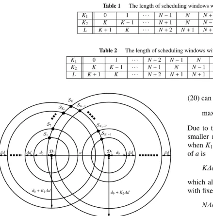
Tables 1 and 2 show the detailed evaluation ofK1,K2andL for even and oddK, respectively. From Table 1 we can see that there are totalM =N+1 kinds of differentLfor even K =2N, among which the least length occurs at K1 =N.
From Table 2 we know that there are total M = N kinds of differentLfor oddK = 2N−1, among which the least length occurs at K1 = N−1 andK1 = N. So there are M = bK/2c+1 different values ofLfor a general K. The minimum ofLisN+1 =dK/2e+1 for both tables, which shows the least length of scheduling window for the pro- posed scheme. All other values of LfromN+2 toK+1 have two combinations ofK1andK2. The maximum ofLis K+1, which occurs atK1=0 orK1=K. From the imple- ment viewpoint, a shorter scheduling window implies less complexity, since the shift register can use a smaller length.
By choosing proper value ofK1, the proposed scheme can be adaptive to variant implementation requirements.
4. Feasibility in the Euclidean Space
We analyze the feasibility of the above PD-based scheme by giving the conditions of node placement in the Euclidean space. For simplicity, constant propagation speed (v) is as- sumed. Denote the distance betweenD1andD2asa. The distance betweenS1andD1is initialized asd0=vτ0, where τ0is any positive value indicating the reference PD. The dis- tance increase step is denoted by∆d =vs∆τ > 0, wheres is a scaling factor and∆τis the PD gap which has been nor- malized in the above model.
Figure 1 is used for demonstration. Denote the cir- cle/sphere centered atDjwith radiusdbyOj(d). The most inner circles/spheres have a radius ofd0, while the increase step of radius is∆d. The most outer circle/sphere aroundD1 andD2 has a radius ofd0+K1∆dandd0+K2∆d, respec- tively. The positions of all source nodes are also partially
Table 1 The length of scheduling windows with evenK=2N.
K1 0 1 · · · N−1 N N+1 · · · K−1 K
K2 K K−1 · · · N+1 N N−1 · · · 1 0
L K+1 K · · · N+2 N+1 N+2 · · · K K+1
Table 2 The length of scheduling windows with oddK=2N−1.
K1 0 1 · · · N−2 N−1 N N+1 · · · K−1 K
K2 K K−1 · · · N+1 N N−1 N−2 · · · 1 0
L K+1 K · · · N+2 N+1 N+1 N+2 · · · K K+1
Fig. 1 Feasibility demonstration forK×2 XC with arbitrary integers 0≤K1≤KandK2=K−K1.
shown by the cross points of related circles/spheres. Fig- ure 1 only shows one possible candidate choice of the source nodes in the upper part. Indeed, the intersection points of the relative circles in the lower part are also feasible for the source nodes in the two-dimensional Euclidean space. So there might be many combinations of the node placement.
In the three-dimensional Euclidean space, the intersection of the relative spheres is a circle. Because any point on the intersection circle is feasible for a source node, the number of combinations of the node placement can be large enough as long as the intersection circle has a positive radius and enough high resolution. WhenK1 =0 orK2=0, there will be only one circle/sphere aroundD1orD2respectively, on which all source nodes are located.
The feasibility condition of the proposed scheme re- quires that the most outer circles/spheres centered at D1 must have at least one intersection point with the most inner circles/spheres centered atD2, and vice versa. Mathemati- cally, we have:∀K1=0,· · ·,Kand∀K2=K−K1
O1(d0+K1∆d) ∩ O2(d0) , ∅
O1(d0) ∩ O2(d0+K2∆d) , ∅ (19) which can be further expressed withaas
a−d0 ≤ d0+K1∆d ≤ a+d0
a−d0 ≤ d0+K2∆d ≤ a+d0
(20) After some computations, the above feasibility condition
(20) can be simplified as
max(K1,K2)∆d≤a≤2d0+min(K1,K2)∆d (21) Due to the relationship K2 = K −K1, we can see that a smaller max(K1,K2) has a wider range of a. Especially, whenK1 =0 orK2 =0, with fixed∆d the narrowest range ofais
K∆d≤a≤2d0 (22)
which also implies that ∆d ≤ 2d0/K. On the other hand, with fixed∆dthe widest range ofais
N∆d≤a≤2d0+N∆d (23)
for evenK=2NwithK1=K2=Nand
N∆d≤a≤2d0+(N−1)∆d (24) for oddK=2N−1 withK1 =NorK2=N. Since there is no other constraint on∆din (23), theoretically it can be any positive value. With properd0and∆d, the distance between D1 andD2 can be determined as required. However, with odd K =2N−1, the feasibility condition (24) implies that
∆d ≤2d0, which limits the upper bound onato be 2Nd0 = (K+1)d0. In this sense, evenKis more preferred than odd K. Other choice ofK1between 0 andKprovides a trade-off between the narrowest and widest ranges ofa. By flexibly adjustingK1,d0and∆d(equivalently the frame length∆τ), the feasibility condition (21) can be widely practical.
Examples: For underwater acoustic applications, we can set parameters asv =1500m/s andd0 =1000m. Two examples are given below.
(i) For a 10×2 XC with K1 = 0 or K1 = 10, the feasibility condition is 10∆d ≤ a ≤ 2d0 = 2000m, which gives the narrowest range ofaand implies that∆d≤200m.
On the other hand, withK1 =5, the feasibility condition is 5∆d≤a≤2d0+5∆d=2000+5∆d, which gives the widest range ofawith arbitrarily value of∆d>0.
(ii) For a 9×2 XC with K1 = 0 orK1 = 9, the fea- sibility condition is 9∆d ≤a ≤2d0 =2000m, which gives the narrowest range of aand implies that ∆d ≤ 2000/9m.
On the other hand, with K1 = 5 orK2 = 5, the feasibility condition is 5∆d ≤ a ≤ 2d0+4∆d = 2000+4∆d, which gives the widest range ofawith∆d≤2d0=2000m.
Moreover, when a suboptimaln(i.e.n>K+1) is con- sidered, we can expect that the feasibility can be greatly im- proved, since there will be more feasible patterns supported
and the alignment conditions can be relaxed to some extent.
For example, withn =K+2, now we have two time-slots for cyclic IA of theKundesired messages, which has many combinations of possible interference grouping for cyclic IA at each destination node, in contrast with the only one com- bination withn=K+1. This provides a trade-offmethod be- tween the multiplexing gain and feasibility in the Euclidean space. When no perfect cyclic IA exists such as in the 3-user X-networks shown in[12], this approach can be expected to make a feasible suboptimal scheme. In fact, when more time slots are involved, more messages besides the original ones are also possible, which compensates the DoF loss in some extent. For example, with one extra time slot, by allowing one more message the maximum DoF of 10/6=5/3 instead of 9/6=3/2 is achieved based on cyclic IA for the three-user X channel in[13].
5. Conclusion
We extended the approach of perfect cyclic IA by PD to K×2 X channels and proposed a general scheme, which is optimal to achieve the DoF of 2K/(K+1). The position of IA can be arbitrarily determined by the parameterK1from time-slot 0 toK along with theK+1 patterns. Feasibility analysis shows that it is widely practical in the Euclidean space. This work generalizes the scope of cyclic IA for X channels in temporal domain.
Acknowledgments
This work was partially supported by the National Natural Science Foundation of China (No. 61271283, U1701265, 61601283, 61472237).
References
[1] V. Cadambe and S. Jafar, “Interference alignment and degrees of freedom of theK-user interference channel,” IEEE Trans. Inf. The- ory, vol.54, no.8, pp.3425–3441, 2008.
[2] V. Cadambe and S. Jafar, “Interference alignment and the degrees of freedom of wirelessXnetworks,” IEEE Trans. Inf. Theory, vol.55, no.9, pp.3893–3908, 2009.
[3] S. Mosleh, J. Ashdown, J. Matyjas, M. Medley, C. Zhang, and L. Liu, “Interference alignment for downlink multi-cell LTE- advanced systems with limited feedback,” IEEE Trans. Wireless Commun., vol.15, no.12, pp.8107–8121, 2016.
[4] W. Shin, M. Vaezi, B. Lee, D.J. Love, J. Lee, and H.V. Poor, “Co- ordinated beamforming for multi-cell MIMO-NOMA,” IEEE Com- mun. Lett., vol.21, no.1, pp.84–87, 2017.
[5] M. Chitre, M. Motani, and S. Shahabudeen, “A scheduling algorithm for wireless networks with large propagation delays,” IEEE Oceans, pp.1–5, 2010.
[6] F.L. Blasco, F. Rossetto, and G. Bauch, “Time interference align- ment via delay offset for long delay networks,” IEEE Trans. Com- mun., vol.62, no.2, pp.590–599, 2011.
[7] M. Chitre, M. Motani, and S. Shahabudeen, “Throughput of net- works with large propagation delays,” IEEE J. Ocean. Eng., vol.37, no.4, pp.645–658, 2012.
[8] F.L. Blasco, F. Rossetto, and G. Bauch, “Time interference align- ment via delay offset for long delay networks,” IEEE Trans. Com- mun., vol.62, no.2, pp.590–599, 2014.
[9] H. Maier, J. Schmitz, and R. Mathar, “Cyclic interference align- ment by propagation delay,” 2012 50th Annual Allerton Conference on Communication, Control, and Computing (Allerton), pp.1761–
1768, IEEE, 2012.
[10] F. Liu, S. Jiang, S. Jiang, and C. Li, “DoF achieving propagation delay aligned structure forK×2 X channels,” IEEE Commun. Lett., vol.21, no.4, pp.897–900, 2017.
[11] S. Jiang, F. Liu, S. Jiang, and X. Geng, “A feasible distance aligned structure for underwater acoustic X networks with two receivers,”
IEICE Trans. Fundamentals, vol.E100-A, no.1, pp.332–334, Jan.
2017.
[12] H. Maier and R. Mathar, “Cyclic interference alignment and cancel- lation in 3-user X- networks with minimal backhaul,” Information Theory Workshop, pp.87–91, 2014.
[13] F. Liu, S. Wang, S. Jiang, and Y. Xu, “Propagation-delay based cyclic interference alignment with one extra time-slot for three-user X channel,” IEICE Trans. Fundamentals, vol.E102-A, no.6, pp.854–
859, June 2019.