AnalysisandDesignofAggregateDemandResponseSystemsBasedonControllability PAPER

(1)

PAPER

Analysis and Design of Aggregate Demand Response Systems Based on Controllability

Kazuhiro SATO^†a)andShun-ichi AZUMA^††b),Members

SUMMARY We address analysis and design problems of aggregate demand response systems composed of various consumers based on controllability to facilitate to design automated demand response machines that are installed into consumers to automatically respond to electricity price changes. To this end, we introduce a controllability index that expresses the worst-case error between the expected total electricity consumption and the electricity supply when the best electricity price is chosen. The analysis problem using the index considers how to maximize the controllability of the whole consumer group when the consumption characteristic of each consumer is not fixed. In contrast, the design problem considers the whole consumer group when the consumption characteristics of a part of the group are fixed. By solving the analysis problem, we first clarify how the controllability, average consumption characteristics of all consumers, and the number of selectable electricity prices are related. In particular, the minimum value of the controllability index is determined by the number of selectable electricity prices. Next, we prove that the design problem can be solved by a simple linear optimization. Numerical experiments demon- strate that our results are able to increase the controllability of the overall consumer group.

key words: aggregate demand response, controllability, real-time pricing

1. Introduction

Real-time pricing (RTP) in smart grids is a mechanism that controls the total electricity consumption by changing the electricity price frequently to reduce the high peaks of total electricity consumption[1]–[7]. RTP systems are usually implemented as feedback systems composed of electricity suppliers, an electricity price decision maker, and a large number of consumers composed of various residential loads, as illustrated in Fig. 1. The electricity price is decided by comparing the total electricity consumption with the electricity supply. The major challenges in RTP are how to determine the electricity prices[8]–[11]and the stability of the feedback system[12]–[14].

To implement RTP, in addition to the above tasks, an important issue is controllability such as electricity price elasticity used in[15]–[22]of a given consumer group, not each consumer. This is because even if there are some consumers with high controllability, a group of all consumers

Manuscript received July 30, 2020.

Manuscript revised November 12, 2020.

Manuscript publicized December 1, 2020.

†The author is with the Department of Mathematical Informat- ics, Graduate School of Information Science and Technology, The University of Tokyo, Tokyo, 113-8656 Japan.

††The author is with the Graduate School of Engineering, Na- goya University, Nagoya-shi, 464-8603 Japan.

a) E-mail: [email protected] b) E-mail: [email protected]

DOI: 10.1587/transfun.2020EAP1093

Fig. 1 Real-time pricing system.

may have low controllability (e.g., most consumers do not pay attention to electricity price changes except for few consumers). That is, if the controllability of a consumer group is low, RTP cannot control the total electricity consumption.

Such controllability can be adjusted by using automated demand response (ADR) machines that are installed into consumers composed of various residential loads to automatically respond to electricity price changes[23]–[29]. How- ever, the existing controllability concept used in[15]–[22]is not adequate to provide a design principle of ADR machines for maximizing the controllability, although it is useful to construct a mathematical model of consumers and to design electricity prices. That is, it is desired to introduce another controllability concept which facilitates to design ADR machines. To the best of our knowledge, only[30],[31]provide such controllability concept. However, these studies assume that each consumer’s consumption is in an on or off state.

Hence, we cannot use the controllability indices proposed in [30],[31]for more general consumers.

For this reason, we introduce a novel controllability index that is suitable for a consumer group composed of such general consumers, and consider a maximization of controllability of a consumer group, not each consumer. To this end, we formulate two problems using the index for maximizing the controllability. The first problem considers how to maximize the controllability of the whole consumer group when the consumption characteristic of each consumer is not fixed. In contrast, the second problem considers the whole consumer group when the consumption characteristics of a part of the group are fixed. Solutions to the second problem will provide the design principles for ADR machines.

The contributions of this paper are summarized as follows: By solving the first problem, we clarify how the controllability, average consumption characteristics of consumers, and the number of selectable electricity prices are related. In particular, we show that the minimum value of the controllability index is determined by the number of selectable electricity prices in the system. We also prove Copyright © 2021 The Institute of Electronics, Information and Communication Engineers

(2)

whole consumer group.

The remainder of this paper is organized as follows.

Section 2 defines an aggregate demand response system and the controllability index of the system. Moreover, we formulate analysis and design problems for system controllability maximization. Section 3.1 provides a solution to the analysis problem. In Sect. 3.2, we show that the design problem can be transformed into a simple linear optimization problem.

Section 4 demonstrates that our results increase the controllability of the whole group. The conclusion is presented in Sect. 5.

Notation: The set of real numbers is denoted by R.

The symbols0_n ∈ Rⁿ and1_n ∈ Rⁿ are column vectors of all zeros and ones, respectively. For any real numbera,|a| denotes the absolute value ofa. The symbols E(A|B)and V(A|B)are the expectation and variance of AassumingB, respectively.

2. Problem Formulations

This section introduces a mathematical model of consumers and a novel controllability concept of an aggregate demand response system composed of consumers. Moreover, in this section, we formulate analysis and design problems.

2.1 Consumer Model

We consider an aggregate demand response system composed ofNconsumers, as illustrated in Fig. 2. This system corresponds to that of the consumer group of the RTP system illustrated in Fig. 1. Each consumer is modeled based on the following perspectives.

1. Electricity consumption of each consumer has a time varying pattern. This pattern can be obtained through statistic studies. Thus, it is sufficient to consider a consumer model at an important time for performing RTP. Here, the important time means the time for total electricity consumption to be a high peak.

2. Electricity consumption of each consumer can be normalized by the maximum consumption among all consumers. Thus, it is sufficient to consider the case that electricity consumption of each consumer is in [0,1].

3. Electricity consumption of each consumer is a random variable, because it is different at an important time for RTP in different days. The random variables are independent from each other, because an electric usage of each consumer does not depend on those of other consumers.

4. Although the average of electricity consumption of each consumer under a fixed electricity price is known, the probability distribution is assumed to be unknown. This is because the identification of the probability distribution is more difficult than that of the average.

Fig. 2 Aggregate demand response system.

5. Each consumer’s electricity price elasticity is different.

We can find consumer models in[30]–[32]based on 2), 3), and 5), although a probability distribution of each electricity consumption is known, that is, 4) is not satisfied in [30]–[32]. In fact, electricity consumption of each consumer in[30]–[32]is a random variable and takes 0 or 1. The value is probabilistically determined by an electricity price elasticity which is different among different consumers. Moreover, [30],[31]modeled consumers based on 1), while[32]did not. That is, the following consumer model in this paper is more realistic than those used in [30]–[32]in senses of possible values of electricity consumption and the setting without assuming the exact identification of a probability distribution of individual electricity consumption.

In Fig. 2, the input is electricity price u ∈ {u1,u2, . . . ,um} at the important time for performing RTP, where mis a fixed positive number, and the output is the individual electricity consumption x_i that takes a value in [0,1] from the perspective 2) at the important time, where u₁,u₂, . . . ,u_mare selectable electricity prices such that

0<u_m<u_m−1 <· · ·<u₁ <∞. (1) From the perspective 3), individual electricity consumption x_iis a random variable andx₁,x₂, . . . ,x_N are independent.

The total electricity consumption of N consumers at the important time is given by

y:=x₁+x₂+· · ·+x_N ∈[0,N]. (2) The relation betweenx_ianduis given by

E(x_i|u=uj)=x¯i j, (3) where ¯x_{i j} (j=1,2, . . . ,m)denotes the consumption behavior of consumerithat is assumed to be known based on the perspective 4), and satisfy

¯

x_i1 ≤x¯_i2 ≤ · · · ≤ x¯_im (4)

that is consistent with the consumer buying behavior subject to (1); that is, if electricity price u is higher, the individual levels of electricity consumption x_i (i = 1,2, . . . ,N) are lower. Moreover, for a fixed j ∈ {1,2, . . . ,m}, ¯x_{i j} is different for each i ∈ {1,2, . . . ,N}, in general. This corresponds to the perspective 5). Because ¯x_{i j} is a characteristic of consumeri, we call ¯xi j (j = 1,2, . . . ,m) thecon- sumption characteristicsof consumeri, and the vectorx¯ :=

(x¯₁₁,x¯₂₁, . . . ,x¯_N1,x¯₁₂,x¯₂₂, . . . ,x¯_N2, . . . ,x¯_1m,x¯_2m, . . . ,x¯N m) ∈

(3)

Fig. 3 Example of a probability density function ofysuch that even if

|E(y|u=u⁰)−r|=0 holds,|y−r|is large.

Fig. 4 Probability density function ofywhen the number of consumers Nis sufficiently large.

[0,1]^{N m}thecollective consumption characteristic.

2.2 Controllability Index

The aim of RTP is to adjust the total electricity consumption, not individual electricity consumption of each consumer. From this perspective, we introduce the following controllability index:

C(x)¯ := max

r∈[0,N] min

u⁰∈ {u1,...,um}

|E(y|u=u⁰)−r|

N . (5)

This index represents the maximum difference between the expected total electricity consumption y and reference r when the bestuis chosen. From this definition, it follows that ifC(x)¯ is smaller (larger), the consumer group has a higher (lower) controllability. Note that controllability index (5) is different from those in [30],[31] which defined by using probability distributions of electricity consumption of consumers.

One might consider that even if|E(y|u =u⁰)−r|is small, the actual total electricity consumption y may be different from referencer. This is because small|E(y|u = u⁰)−r|does not mean thaty≈ris true, e.g., in the case of Fig. 3. However, it is not true ifNis sufficiently large. In fact, Theorem 3 in Appendix B guarantees that the probability distribution of the random variable y under u = u⁰ can be approximated as a Gaussian distribution with expectation E(y|u=u⁰), as shown in Fig. 4. Thus, if|E(y|u=u⁰)−r|= 0 holds,|y−r|is likely to be small. For this reason,C(x)¯ is a reasonable index of the controllability.

The following example illustrates controllability index C(x)¯ in a concrete situation.

Example 1: Consider a consumer group where N =

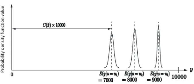
Fig. 5 Probability density functions ofywhenE(y|u=u1)=7,000, E(y|u=u2)=8,000, andE(y|u=u3)=9,000.

Fig. 6 Probability density functions ofywhenE(y|u=u1)=2,000, E(y|u=u2)=7,000, andE(y|u=u3)=8,000.

10,000 and m = 3, and assume that the probability density functions of ywith respect tou₁,u₂, andu₃are given as shown in Fig. 5. Then, we obtainC(x)¯ =0.7, because minu⁰∈ {u1,u2,u3} |E(y|u=u⁰)−r|

10,000 takes the maximum value 0.7 whenr=0, as shown in Fig. 5. In contrast, when the probability density functions of y are given as shown in Fig. 6, we haveC(x)¯ =0.25, because min_u⁰_{∈ {u}₁_,u₂_,u₃} |E(y|u=u⁰)−r|

10,000

takes the maximum value 0.25 whenr=4,500, as shown in

Fig. 6.

2.3 Analysis and Design Problems

It is desirable for controllability indexC(x)¯ to be small (i.e., for the controllability of a consumer group to be high), if we implement RTP. This is because if the controllability is high, we can reduce the high peak of total electricity consumption by changing the electricity price. To characterize such consumer groups, we consider the following analysis problem.

Problem 1: Find a collective consumption characteristic

¯

x∈[0,1]^{N m}that minimizes controllability indexC(x).¯ In Problem 1, none of the consumption characteristics ¯x_{i j}are fixed. In this particular model, all consumers are treated as an electric device equipped with an ADR machine[23]–[29].

That is, we can freely set the consumption characteristics of all consumers. However, in a practical situation, there are electric devices such as refrigerators with fixed consumption characteristics.

For this reason, we also consider the following design problem.

(4)

1,2, . . . ,n, j = 1,2, . . . ,m) of n consumers minimiz- ing controllability indexC(x).¯

Remark 1: Problems 1 and 2 can be formulated as linear programming problems directly using (5). However, we cannot solve the problems in a practical time if the number of consumers N is considerably large. Thus, in the next section, we simplifyC(x)¯ in (5) for solving Problems 1 and 2 in the cases thatNis considerably large.

3. Solution to Problems 1 and 2

3.1 Solution to Problem 1

This subsection derives the solution to Problem 1 using the consumer group characteristic.

We first characterize controllability indexC(x). It fol-¯ lows from (2) and (3) that

E(y|u=uj)=E(

N

X

i=1

xi|u=uj)=

N

X

i=1

¯

xi j. (6) Furthermore, from (4), (6), and ¯x_{i j} ∈[0,1], we have that

0≤E(y|u=u1)≤ · · · ≤ E(y|u=um)≤N. (7) We define













d₀(x)¯ :=E(y|u=u₁), d_m(x)¯ :=N−E(y|u=u_m), d_k(x)¯ :=Ê(y^|u⁼û^k⁺¹⁾₂^−E(y^|u⁼û^k⁾,

(8)

wherek=1,2, . . . ,m−1, such that

d₀(x)¯ +2d1(x)¯ +· · ·+2dm−1(x)¯ +d_m(x)¯ =N, (9) as illustrated in Fig. 7. Here, d0(x),¯ d1(x), . . . ,¯ d_m(x)¯ are nonnegative for any ¯x∈[0,1]^{N m}, because (7) holds. Using the functions in (8), the following lemma is obtained.

Lemma 1: (i) ForC(x)¯ in (5), C(x)¯ = 1

N max

k∈ {0,1,...,m}d_k(x).¯ (10)

(ii) For every ¯x∈[0,1]^{N m},

C(x¯^∗)≤C(x)¯ (11)

Fig. 7 Illustration of (8).

Proof : First, we prove (i). Let

y¯_j :=E(y|u=u_j). (13)

From (5) and (13), minu⁰∈ {u1,u2,...,um}|E(y|u = u⁰)−r| = minj∈ {1,2,...,m}|y¯_j−r|holds, and thusC(x)¯ is rewritten as

C(x)¯ = max

r∈[0,N] min

j∈ {1,2,...,m}

|y¯_j−r|

N . (14)

Furthermore, it follows from (7) and (13) that 0≤ y¯₁+y¯₂

2 ≤ y¯₂+y¯₃

2 ≤ · · · ≤ y¯_m−1+y¯_m

2 ≤N,

and we thus have

[0,N]=S₁∪S₂∪ · · · ∪S_m (15) for

S₁:=[0, y¯₁+y¯₂

2 ], S_m:=[y¯_m−1+y¯_m

2 ,N], (16)

S_k :=[y¯_k−1+y¯_k

2 , y¯_k+y¯_k+1

2 ] (k=2,3, . . . ,m−1).

Hence, (14), (15), (16), and (A·1) in Appendix A yield that C(x)¯ = 1

N max

k∈ {1,...,m} max

r∈Sk

j∈ {1,...,m}min |y¯_j−r|

!

. (17)

Because maxr∈Sk

j∈ {1,2,...,min m}|y¯_j−r|=max

r∈Sk

|y¯_k−r| (18) (which is illustrated in Fig. 8), the right-hand side of (17) is equivalent to

1

N max

k∈ {1,2,...,m} max

r∈Sk

|y¯_k −r|

!

. (19)

Using (13), (16), and (A·2) in Appendix A, for eachk ∈ {1,2, . . . ,m}, max

r∈Sk

|y¯_k−r|in (19) can be transformed into maxr∈Sk

|y¯_k−r|= max

i∈ {k−1,k}di(x),¯ (20)

whered_k(x)¯ is defined as (8). From (17), (19), and (20), we obtain that

C(x)¯ =1

N max

k∈ {1,2,...,m} max

i∈ {k−1,k}di(x)¯

!

=1

N max

k∈ {0,1,...,m}d_k(x).¯ Thus,C(x)¯ is given by (10).

Next, we prove (ii). Suppose that (11) holds for all

¯

x∈[0,1]^{N m}. Then,

(5)

Fig. 8 Illustration of (18).

C(x¯^∗)≤ 1

2m (21)

because ¯x_{i j} = ²_2m^j−1 (i =1,2, . . . ,N,j =1,2, . . . ,m)yields C(x)¯ = _2m¹ . From (10) and (21), maxk∈ {0,1,...,m}d_k(x¯^∗) ≤

N

2m, and thus d_k(x¯^∗)≤ N

2m (k=0,1, . . . ,m). (22) It follows from (9) and (22) that (12) holds. Conversely, suppose that (12) holds and ¯xminimizesC(x). If there exists¯ i∈ {0,1, . . . ,m}such thatd_i(x)¯ ≤d_i(x¯^∗)=d₀(x¯^∗), (9) and (iii) in Appendix A imply that there exists j ∈ {0,1, . . . ,m}

satisfying j,isuch thatd_j(x)¯ ≥d_j(x¯^∗)=d₀(x¯^∗). Hence, (10) yieldsC(x)¯ ≥C(x¯^∗). However, because ¯xminimizes C(x), i.e.,¯ C(x)¯ ≤C(x¯^∗), we obtain that

C(x)¯ =C(x¯^∗), (23)

which means that (11) holds for all ¯x∈[0,1]^{N m}. Statement (i) of Lemma 1 means thatC(x)¯ is characterized by the (half of) distances between two adjacent points in 0,E(y|u = u₁),E(y|u = u₂), . . . ,E(y|u = u_m), and N, as shown in Fig. 7. Statement (ii) means that the consumer group has the highest controllability if and only if the distances are equal. For example, Fig. 9 illustrates the probability density functions of y when (12) holds under m = 4. Then,C(x)¯ takes the minimum value ¹₈. This is because if (12) does not hold,C(x)¯ becomes larger than ¹₈ as with the case shown in Fig. 10.

Next, we express the solution to Problem 1 using average consumption characteristics. It follows from (8) that (12) can be transformed into

E(y|u=u_j)= 2j−1

2m N (j =1,2, . . . ,m). (24) Substituting (6) into (24), we have that

1 N

N

X

i=1

¯

x_{i j} =2j−1

2m (j=1,2, . . . ,m). (25) Thus, Lemma 1 and (25) imply the following theorem.

Theorem 1: (i) A collective consumption characteristic ¯x minimizes controllability index C(x)¯ if and only if (25) holds.

(ii) The minimum value ofC(x)¯ is given by_2m¹ . Theorem 1 clarifies how the controllability, average consumption characteristic of all consumers, and number

Fig. 9 Probability density functions ofywhen (12) holds underm=4.

Fig. 10 Probability density functions ofywhen (12) does not hold under m=4.

of electricity prices are related. In fact, (i) means that the consumer group with the maximum controllability can be characterized using the average consumption characteristic of all consumers. Furthermore, (ii) shows that the minimum value of C(x)¯ is determined by the number of selectable electricity prices.

3.2 Solution to Problem 2

This subsection shows that Problem 2 can be solved using a simple linear optimization problem. Such solutions are not trivial, because Theorem 1 implies that if there exists

j ∈ {1,2, . . . ,m}such that XN

i=n+1

¯

xi j >2j−1

2m N, (26)

then there exists no collective consumption characteristic ¯x satisfyingC(x)¯ =_2m¹ . To solve Problem 2 even if (26) holds, we first transform it into the following linear optimization problem:

minimize f(X,¯ t):=t (27)

subject to AX¯ +B≤t1_m+1,

EX¯ ≤0n(m−1), 0nm≤X¯ ≤1nm,

where the symbol ≤ denotes elementwise inequal- ity, X¯ :=

¯

x^T₁ x¯^T₂ · · · x¯^T_mT

∈ R^nm, x¯_j :=

x¯₁_j x¯_2j · · · x¯_{n j}T

∈Rⁿ (j =1,2, . . . ,m), and

(6)

Table 2 Second example of average consumption characteristics of N−nconsumers with fixed consumption characteristics.

j 1 2 3 4 5 6 7 8 9 10

1 N−n

PN

i=n+1x¯i j 0.60 0.65 0.70 0.75 0.80 0.85 0.90 0.93 0.94 0.97

A:=

* . . . . . . . . . ,

1^T_n

−¹^Tⁿ

2 1^T_n

. .. ...2

−¹^Tⁿ

2 1^T_n

2

−1^T_n + / / / / / / / / / -

∈R^(m+1)×nm,

B:=

* . . . . . . . . . . ,

PN k=n+1x¯k1 PN

k=n+1(x¯k2−x¯k1) 2...

PN

k=n+1(x¯k m−x¯k(m−1)) 2

N−PN k=n+1x¯_km

+ / / / / / / / / / / -

∈R^m+1,

E:=

* . . . . . ,

I_n −I_n I_n −I_n

. .. ...

I_n −I_n + / / / / / -

∈R^n(m−1)×nm.

The proof that Problem 2 is equivalent to problem (27) is given in Appendix C. Note that it follows from (A·10) in Appendix C that

C(x)¯ = t

N. (28)

Because problem (27) is a linear optimization problem, it can be solved using standard solvers such as the MATLAB linprog command. However, ifnis large, it becomes difficult to numerically solve problem (27), because the number of the optimization variables(X,¯ t)of problem (27) is equal to nm+1.

To solve Problem 2 with largen, we consider the following linear optimization problem:

minimize g(Z,t):=t (29)

subject to AZ˜ +B≤t1_m+1,

E Z˜ ≤0m−1, 0_m≤Z ≤n1_m,

where ˜Aand ˜Ecorrespond to AandEin the case ofn=1, respectively, and Z :=

Z₁ Z₂ · · · Z_mT

∈R^m. Note that the number of optimization variables(Z,t)of problem (29) is equal tom+1. Thus, we can solve problem (29) more efficiently than problem (27).

The optimal value of problem (29) is less than or equal to that of problem (27). In fact, if(X,¯ t)is a globally optimal solution to problem (27), then (Z,t) with Zj = Pn

i=1x¯i j

satisfies the constraint condition of problem (29). We thus obtain the following theorem.

Theorem 2: Let (Z,t) be a globally optimal solution to problem (29). Then, ¯x_{i j} (i = 1,2, . . . ,n, j = 1,2, . . . ,m) satisfying







 Pn

i=1x¯_{i j} =Z_j,

0≤x¯_i1 ≤x¯_i2 ≤ · · · ≤x¯_im≤1 (30) is a globally optimal solution to Problem 2, and (28) holds.

Proof : Because (Z,t) satisfies the constraint of problem (29), (X,¯ t) satisfies that of problem (27). Furthermore, because the optimal value of problem (29) is less than or equal to that of problem (27), (X,¯ t) is a globally optimal

solution to problem (27).

From Theorem 2, we can easily obtain a globally optimal solution to Problem 2 by solving problem (29). In fact, if(Z,t)is a globally optimal solution to problem (29), then

¯

x₁_j =x¯_2j =· · ·=x¯_{n j}= 1

nZ_j (j=1,2, . . . ,m) (31) implies that ¯x_{i j} (i = 1,2, . . . ,n, j = 1,2, . . . ,m) satisfies (30). This facilitates to design ADR machines for maximizing the controllability subject to the existences of fixed consumption characteristics.

4. Numerical Experiments

This section demonstrates that as the number of consumers nwith non-fixed consumption characteristics increases, we can increase the controllability of the whole consumer group.

That is, we show that asnincreases, we can decrease controllability indexC(x)¯ by appropriately designing ¯x. This is because Problem 2 is equivalent to (A·9), which means that C(x)¯ is able to be lower for largern, in Appendix C.

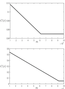
To this end, we suppose that the numbers of consumers in the consumer group and electricity prices are 10⁶ and 10, respectively, i.e., N = 10⁶ andm =10. Furthermore, we assume that Tables 1 and 2 illustrate two examples of the average consumption characteristics ofN−nconsumers with fixed consumption characteristics. Note that Theorem 1 implies thatC(x)¯ ≥ ¹

2m =0.05 for any ¯x∈[0,1]^{N m}. The top and bottom of Fig. 11 show the relationship between n andC(x)¯ for the average consumption characteristics of N −n consumers listed in Tables 1 and 2, respectively. Here, we adopted a solution to Problem 2 as ¯xi j

(7)

Fig. 11 Relationship betweennandC(x)¯ for the average consumption characteristics ofN−nconsumers listed in Tables 1 (top) and 2 (bottom).

(i=1,2, . . . ,n,j=1,2, . . . ,m), and obtained the solution by solving linear optimization problem (29), as stated in Theo- rem 2. According to Fig. 11, asnincreases,C(x)¯ decreases.

The difference between the top and bottom of Fig. 11 is the minimumnat which the consumer groups have maximum controllability. This comes from the difference in the average consumption characteristic ofN −nconsumers with the fixed consumption characteristics, as shown in Tables 1 and 2. That is, when the controllability of consumers with fixed consumption characteristics is low, more consumers with non-fixed consumption characteristics are required to achieve high controllability.

5. Conclusion

We presented two controllability maximization problems of aggregate demand response systems, one in which all consumers had variable consumption characteristics and one in which the consumption characteristics of some consumers was fixed. The problems were formulated using the controllability index. Formulating the first problem enabled us to clarify how the controllability, average consumption characteristics of all consumers, and the number of selectable electricity prices are related. Moreover, we proved that solutions to the second problem are given by solving a simple linear optimization problem. Furthermore, we demonstrated through numerical experiments that our results are able to increase the controllability of the whole consumer group.

Acknowledgments

This work was supported by JST CREST Grant Number JP-

MJCR15K1 and Japan Society for the Promotion of Science KAKENHI under Grant 20K14760.

References

[1] M.H. Albadi and E.F. El-Saadany, “A summary of demand response in electricity markets,” Electric Power Systems Research, vol.78, no.11, pp.1989–1996, 2008.

[2] M. Alizadeh, X. Li, Z. Wang, A. Scaglione, and R. Melton, “Demand- side management in the smart grid: Information processing for the power switch,” IEEE Signal Process. Mag., vol.29, no.5, pp.55–67, 2012.

[3] M. Jin, W. Feng, C. Marnay, and C. Spanos, “Microgrid to enable optimal distributed energy retail and end-user demand response,”

Applied Energy, vol.210, pp.1321–1335, 2018.

[4] T. Logenthiran, D. Srinivasan, and T.Z. Shun, “Demand side management in smart grid using heuristic optimization,” IEEE Trans.

Smart Grid, vol.3, no.3, pp.1244–1252, 2012.

[5] A.H. Mohsenian-Rad and A. Leon-Garcia, “Optimal residential load control with price prediction in real-time electricity pricing environ- ments,” IEEE Trans. Smart Grid, vol.1, no.2, pp.120–133, 2010.

[6] E. Shirazi and S. Jadid, “Optimal residential appliance scheduling under dynamic pricing scheme via hemdas,” Energy and Buildings, vol.93, pp.40–49, 2015.

[7] M. Ye and G. Hu, “Game design and analysis for price-based demand response: An aggregate game approach,” IEEE Trans. Cybern., vol.47, no.3, pp.720–730, 2017.

[8] K. Ma, G. Hu, and C.J. Spanos, “Distributed energy consumption control via real-time pricing feedback in smart grid,” IEEE Trans.

Control Syst. Technol., vol.22, no.5, pp.1907–1914, 2014.

[9] L.P. Qian, Y.J. A. Zhang, J. Huang, and Y. Wu, “Demand response management via real-time electricity price control in smart grids,”

IEEE J. Sel. Areas Commun., vol.31, no.7, pp.1268–1280, 2013.

[10] P. Samadi, H. Mohsenian-Rad, R. Schober, and V.W. S. Wong, “Ad- vanced demand side management for the future smart grid using mechanism design,” IEEE Trans. Smart Grid, vol.3, no.3, pp.1170–

1180, 2012.

[11] N.Y. Soltani, S.-J. Kim, and G.B. Giannakis, “Real-time load elasticity tracking and pricing for electric vehicle charging,” IEEE Trans.

[12] S. Izumi and S. Azuma, “Real-time pricing by data fusion on networks,” IEEE Trans. Ind. Informat., vol.14, no.3, pp.1175–1185, 2018.

[13] M. Roozbehani, M.A. Dahleh, and S.K. Mitter, “Volatility of power grids under real-time pricing,” IEEE Trans. Power Syst., vol.27, no.4, pp.1926–1940, 2012.

[14] X. Zhang and A. Papachristodoulou, “A real-time control framework for smart power networks: Design methodology and stability,”

Automatica, vol.58, pp.43–50, 2015.

[15] H.A. Aalami, M.P. Moghaddam, and G.R. Yousefi, “Demand response modeling considering interruptible/curtailable loads and ca- pacity market programs,” Applied Energy, vol.87, no.1, pp.243–250, 2010.

[16] M. Asensio and J. Contreras, “Risk-constrained optimal bidding strat- egy for pairing of wind and demand response resources,” IEEE Trans.

[17] S. Fan and R.J. Hyndman, “The price elasticity of electricity demand in South Australia,” Energy Policy, vol.39, no.6, pp.3709–

3719, 2011.

[18] H. Jalili, M.K. Sheikh-El-Eslami, M.P. Moghaddam, and P. Siano,

“Modeling of demand response programs based on market elasticity concept,” J. Ambient Intell. Human. Comput., vol.10, no.6, pp.2265–

2276, 2019.

[19] R. Lu, S.H. Hong, and X. Zhang, “A dynamic pricing demand response algorithm for smart grid: Reinforcement learning approach,”

Applied Energy, vol.220, pp.220–230, 2018.

(8)

constrained unit commitment problem with demand response,” IEEE Trans. Smart Grid, vol.9, no.2, pp.1175–1183, 2018.

[22] C. Yang, C. Meng, and K. Zhou, “Residential electricity pricing in China: The context of price-based demand response,” Renewable and Sustainable Energy Reviews, vol.81, pp.2870–2878, 2018.

[23] S. Althaher, P. Mancarella, and J. Mutale, “Automated demand response from home energy management system under dynamic pricing and power and comfort constraints,” IEEE Trans. Smart Grid, vol.6, no.4, pp.1874–1883, 2015.

[24] S. Azuma, T. Nakamoto, S. Izumi, T. Kitao, and I. Maruta, “Random- ized automated demand response for real-time pricing,” 6th IEEE PES Conference on Innovative Smart Grid Technologies, 2015.

[25] M. Kolenc, N. Ihle, C. Gutschi, P. Nemček, T. Breitkreuz, K. Goed- derz, N. Suljanović, and M. Zajc, “Virtual power plant architecture using OpenADR 2.0b for dynamic charging of automated guided ve- hicles,” International Journal of Electrical Power & Energy Systems, vol.104, pp.370–382, 2019.

[26] A.H. Mohsenian-Rad, V.W.S. Wong, J. Jatskevich, R. Schober, and A. Leon-Garcia, “Autonomous demand-side management based on game-theoretic energy consumption scheduling for the future smart grid,” IEEE Trans. Smart Grid, vol.1, no.3, pp.320–331, 2010.

[27] D.H. Nguyen, S. Azuma, and T. Sugie, “Novel control approaches for demand response with real-time pricing using parallel and distributed consensus-based ADMM,” IEEE Trans. Ind. Electron., vol.66, no.10, pp.7935–7945, 2019.

[28] X. Yang, G. Wang, H. He, J. Lu, and Y. Zhang, “Automated demand response framework in ELNs: Decentralized scheduling and smart contract,” IEEE Trans. Syst., Man, Cybern.,Syst., vol.50, no.1, pp.58–72, 2020.

[29] X. Yang, Y. Zhang, H. Wu, and H. He, “An event-driven ADR approach for residential energy resources in microgrids with uncer- tainties,” IEEE Trans. Ind. Electron., vol.66, no.7, pp.5275–5288, 2019.

[30] K. Sato and S. Azuma, “Controllability analysis of an aggregate demand response system,” Math. Probl. Eng., vol.2015, no.487173, pp.1–11, 2015.

[31] K. Sato and S.-I. Azuma, “Controllability analysis of aggregate demand response system in multiple price-change situation,” IEICE Trans. Fundamentals, vol.E100-A, no.2, pp.376–384, Feb. 2017.

[32] S.M. Krause, S. Börries, and S. Bornholdt, “Econophysics of adap- tive power markets: When a market does not dampen fluctuations but amplifies them,” Phys. Rev. E, vol.92, no.1, p.012815, 2015.

[33] L. Koralov and Y.G. Sinai, Theory of Probability and Random Pro- cesses, Springer, 2007.

[34] S. Boyd and L. Vandenberghe, Convex Optimization, Cambridge University Press, 2004.

Appendix A: Mathematical Formulas We present three formulas to prove Lemma 1.

(i) Let X be a closed set and f : X → R be a map. If X1,X2, . . . ,XnpartitionX, i.e.,X =X1∪X2∪ · · · ∪Xn, then

maxx∈X f(x)= max

i∈ {1,2,...,n} max

x∈Xi

f(x)

!

. (A·1)

(ii) Leta₁,a₂,a₃ ∈Rbe numbers satisfyinga₁ ≤ a₂ ≤a₃. Then, we obtain that

x∈[amax1,a3]

|a2−x|= max

i∈ {1,2}α_i (A·2)

Appendix B: Approximation of y Using a Gaussian Distribution

This appendix explains that if the number of consumers N is sufficiently large, the generalized central limit theorem implies that a probability distribution of y foru = u⁰can be approximated by a Gaussian distribution with expectation E(y|u=u⁰).

A sequence of random variables{X_i}is said to converge in distribution to a random variable X if limn→∞F_n(x) = F(x)for anyx∈Rat whichFis continuous, whereF_nand Fare the distribution functions of random variablesX_nand X, respectively. The following proposition is known as the generalized central limit theorem[33].

Proposition 1: Let{X_i}be a sequence of independent random variables with E(Xi) = µ_i and V(X_i) = σ²_i. Let

A_n:=µ₁+µ₂+· · ·+µ_nandB_n:=q

σ₁²+σ²₂+· · ·+σ²_n. If

n→∞lim 1 B²_n

Xn

i=1

E(|Xi−µ_i|²·1{ |Xi−µi| ≥Bn})=0 (A·3) for any >0, then^X¹^+X²⁺^···_B_n^+Xⁿ^−Aⁿ converges in distribution to the standard Gaussian random variable, where1{ · }denotes

the indicator function.

Note that Proposition 1 guarantees that if (A·3) (called the Lindeberg condition) is satisfied, normalized sums of independent random variables converge in distribution to the standard Gaussian random variable without needing the as- sumption that the random variables are identical.

The following condition is a sufficient condition for (A·3) to hold[33]: There existsδ >0 such that

n→∞lim 1 B^2+δ_n

n

X

i=1

E(|X_i−µ_i|^2+δ)=0. (A·4) In fact, because|X_i−µ_i| ≥B_nyields

Xi−µi

Bn

δ ≥1, for any >0,

1 B²_n

Xn

i=1

E

|X_i−µ_i|²·1_{{ |X}_i_−µ_i_{| ≥B}_n}

≤ 1 B²_n

n

X

i=1

E

X_i−µ_i B_n

δ· |X_i−µ_i|²·1_{{ |X}_i_−µ_i_{| ≥B}_n}

!

≤ 1

^δB_n²^+δ Xn

i=1

E

|X_i−µ_i|^2+δ .

Hence, if (A·4) holds, (A·3) also holds. Here, (A·4) is called the Lyapunov condition.

Using Proposition 1, we can show that if the number of consumersNis sufficiently large, the probability distribution

(9)

of total electricity consumption y foru = u⁰ is close to a Gaussian distribution with expectationE(y|u=u⁰).

Theorem 3: If

Nlim→∞V(y|u=uj)=∞, (A·5)

then ^y−E(y|u=u√ ^j⁾

V(y|u=uj) converges in distribution to the standard Gaussian random variable.

Proof : To prove this claim, we use Lyapunov condition (A·4). Let B_{N j} := q

PN

i=1V(x_i|u=u_j), whereV(x_i|u = u_j) = E(|x_i −E(x_i|u = u_j)|²) = E(|x_i −x¯_{i j}|²). Since xi ∈ [0,1], we have|xi −x¯i j| ≤ 1 for j =1,2, . . . ,m, and thus

N

X

i=1

E(|x_i−x¯_{i j}|³) B³_{N j} ≤

N

X

i=1

E(|x_i−x¯_{i j}|²) B³_{N j} ≤ 1

B_{N j}. (A·6) Because y is defined by (2) and the random variables x₁,x₂, . . . ,x_N are independent,

V(y|u=u_j)=

N

X

i=1

V(x_i|u=u_j)=B²_{N j}. (A·7) Thus, (A·5) holds if and only if limN→∞B_{N j} =∞. Hence, (A·6) implies that if limN→∞V(y|u = uj) = ∞, then limN→∞ 1

B³_{N j}

PN

i=1E(|x_i−x¯_{i j}|³)=0. Therefore, (A·4) with δ=1 holds, and thus (A·3) also holds. Hence, Proposition

1 implies this theorem.

If there exists a positive constantKsuch that

V(x_i|u=u_j)≥K (A·8) for any i ∈ {1,2, . . . ,N} and any j ∈ {1,2, . . . ,m}, then (A·7) yields V(y|u = u_j) ≥ K N. Hence, if (A·8) holds for anyi ∈ {1,2, . . . ,N} and any j ∈ {1,2, . . . ,m}, (A·5) also holds. In practice, we can consider that (A·8) holds for anyi ∈ {1,2, . . . ,N} and any j ∈ {1,2, . . . ,m}. Thus, if N is sufficiently large, V(y|u = u_j) is also sufficiently large. Hence, Theorem 3 guarantees that ifN is sufficiently large, the probability distribution ofy foru =u⁰is close to a Gaussian distribution with expectationE(y|u=u⁰).

Appendix C: Proof of that Problem 2 is Equivalent to Linear Optimization Problem(27) Problem 2 can be described as follows:

minimize C(x)¯ (A·9)

subject to 0≤x¯_i1 ≤ · · · ≤ x¯_im ≤1 (i=1, . . . ,n).

It follows from (6) and (8) that

n

X

i=1

¯ x_i1+

N

X

k=n+1

¯

x_k1=d₀(x),¯

n

X

i=1

(x¯_i(j+1)−x¯_{i j})+

N

X

k=n+1

(x¯_k_(j+1)−x¯_{k j})=2dj(x),¯

−

n

X

i=1

¯

x_im+N−

N

X

k=n+1

¯

x_km=d_m(x).¯

forj=1,2, . . . ,m−1. This is equivalent toAX¯+B=Dwith D:=

d0(x)¯ d1(x)¯ · · · dm(x)¯ T

. Defininga_k andb_k as thek+1-th rows of matricesAandB, respectively, (10) implies that

C(x)¯ = 1

N max

k∈ {0,1,...,m}(a_kX¯ +b_k). (A·10) Thus, problem (A·9) is equivalent to the piecewise-linear minimization problem

minimize max

k∈ {0,1,...,m}(a_kX¯+b_k) (A·11) subject to 0≤x¯_i1 ≤ · · · ≤x¯_im≤1 (i=1, . . . ,n).

By direct calculation, optimization problem (A·11) can be transformed into (27)[34].

Kazuhiro Sato received his B.S., M.S., and Ph.D. degrees from Kyoto University, Japan, in 2009, 2011, and 2014, respectively. He was a Post Doctoral Fellow at Kyoto University from 2014 to 2017. From 2017 to 2019, he was an As- sistant Professor at Kitami Institute of Technol- ogy. He is currently a Lecturer of Department of Mathematical Informatics, Graduate School of Information Science and Technology, The Uni- versity of Tokyo. He is a member of SICE and IEEE. His research interests include mathematical control theory and optimization.

Shun-ichi Azuma received the B.Eng. de- gree in electrical engineering from Hiroshima University, Higashi Hiroshima, Japan, in 1999, and the M.Eng. and Ph.D. degrees in control engineering from Tokyo Institute of Technology, Tokyo, Japan, in 2001 and 2004, respectively.

He is currently a Professor in the Department of Mechanical Systems Engineering, Graduate School of Engineering, Nagoya University, Na- goya, Japan. Prior to joining Nagoya University, he was an Assistant Professor and an Associate Professor in the Department of Systems Science, Graduate School of In- formatics, Kyoto University, Uji, Japan, from 2005 to 2011 and from 2011 to 2017, respectively. He serves as Associate Editors of IFAC Journal Au- tomatica from 2014, IEEE Transactions on Automatic Control from 2019, and so on. His research interests include analysis and control of hybrid systems and applications to systems biology.