Overview of Activities in Stochastic Data Assimilation for Applications in Aerodynamics
Richard P. Dwight Jouke H.S. de Baar Andrea Sciacchitano Mustafa Percin Hester Bijl Fulvio Scarano
Aerodynamics Section, Faculty of Aerospace Engineering, TU Delft, 2600 GB Delft, The Netherlands.
https://aerodynamics.lr.tudelft.nl/~rdwight
Abstract
In this conspectus paper we present a brief summary of a variety of recent activities in data assimilation performed at the Aerodynamics Section of the TU Delft. We hope to demonstrate a few of the exciting possibilities for combining experimental data and numerical models, improving the capability of both. Our activities are bound by a common theme of combining experimental wind-tunnel measurements and CFD simulations in order to (i) improve fidelity of experimental data, (ii) obtain estimates of unmeasured quantities, (iii) estimate modeling error and parametric uncertainty in simulation. The methodologies we use depends strongly on the application, but all have Bayesian inference at their root with some statistical model representing the relation between measurement and simulation. Bayesian statistics offers a coherent and flexible framework for describing solutions of the ill-posed problems that arise in this analysis of data, but new numerical methods are needed to find these solutions efficiently.
Key words: Bayesian inference, uncertainty quantification, data assimilation, aerodynamics, CFD, particle image velocimetry, model inadequacy, Kriging.
Introduction
This paper is intended primarily as an overview of some recent activities of the data assimilation group at the Aerodynamics Section, TU Delft. For technical details see our papers cited throughout. All work has a foundation Bayesian inference. In three sections we discuss three distinct methodologies and applications:
1. Reducing uncertainty in aeroelastic flutter boundaries.
2. Kriging interpolation of stereo-PIV data with a local error estimate.
3. Navier-Stokes simulation in gappy PIV data.
In addition to the activities described in this document, we are also working on at this time (September 2012):
1. Calibration of RANS turbulence models, with a view to obtaining estimates of model inadequacy.
2. Multi-level statistical models for estimating structural variability (Dwight et al., 2012).
3. Kalman smoothing for filling gaps and increasing time resolution of PIV data.
4. Least-squares FEM solutions to the problem of integrating PIV data and CFD solvers (Dwight, 2010).
https://aerodynamics.lr.tudelft.nl/~rdwight
Key words: Bayesian inference, uncertainty quantification, data assimilation, aerodynamics, CFD, particle image velocimetry, model inadequacy, Kriging.
1. Reducing Uncertainty in Aeroelastic Flutter Boundaries
1In this section we compute the uncertainty in dynamic stability boundaries in an aeroelastic system (flutter) due to uncertainties in structural parameters. For moderate levels of structural uncertainty (±5%) we observe extremely high levels of uncertainty in the flutter altitude (±3500 ft) for a model wing. This is a consequence of both high sensitivity of the stability boundary to individual structural parameters, and the cumulative effect of many parameters. We conclude that the predictive capability of our aeroelastic analysis is fundamentally limited by our incomplete knowledge of the structure, more so than by discretization error or modeling inadequacy. To address this limitation we assume measurements of the aeroelastic response at sub-critical altitudes are available, such data as might be gathered from flight-tests. Using Bayesian inference we deduce updated uncertainties for structural parameters and the flutter altitude. Using very small amounts of data we see the introduction of a covariance relationship into the structural parameters and a substantial reduction in flutter boundary uncertainty. In this framework we study the informativeness of sub-critical eigenvalue measurements for the flutter altitude with respect to two parameters: measurement accuracy, and proximity of the measurement to the flutter altitude.
Motivation and Methodology
Flight flutter tests entail cost and risk, whereas computational methods may not accurately predict the flutter boundary (Lind and Brenner, 1997). As such there is a history in aeroelasticity of combining limited flight-test data at sub-critical speeds, with simplified fluid-structure models to predict the flutter envelope, either deterministically (Zimmerman and Weissenburger, 1964) or stochastically (Khalil et al., 2010).
Stochastic approaches arise from the acknowledgement that both estimates of structural parameters and experimental measurements are imprecise. Epistemic uncertainty in the former arises from airframe material and manufacturing variability, as well as wear over varying service histories of aircraft. Recent work has shown that small uncertainties in a large number of structural parameters can result in dramatic uncertainties in the aeroelastic response (Pettit and Beran, 2006; Witteveen et al., 2007) in particular the flutter boundary (Marques et al., 2010). Our goal in this section is to reduce the epistemic uncertainty in both parameters and response using experimental observations of stability eigenvalues of the system at non-flutter conditions. In contrast to previous studies of model updating in aeroelasticity, our model is a high-fidelity fluid-structure interaction (FSI) solver, with a finite-volume compressible Euler solver for the fluid part - which makes the method applicable to the transonic regime. Furthermore since the stand-alone model (without data) is predictive and accurate, we expect the amount of flight-test data required to update the model to be low, and the calibrated model to have broad validity. These benefits justify the extra computational work involved resulting from the high cost of the FSI simulation.
The two main components of the statistical analysis are: 1) propagating specified structural parameter uncertainty through the FSI simulation to obtain estimates of flutter boundary uncertainty, and 2) using experimental data to update estimates of structural uncertainty in the model. The former is accomplished with non-intrusive uncertainty quantification (UQ) techniques (Xiu and Karniadakis, 2002), in particular probabilistic collocation (Loeven, 2010). For the latter we construct a statistical model relating the output of the simulation to the experimental observations, and solve it within the Bayesian framework. There are several benefits to this stochastic approach: the inherent ill-posedness of the inverse problem is treated naturally without need for regularization terms, noise in the experimental observations can be readily accounted for, as can prior information on the structure (Kennedy and O’Hagan, 2001).
Flutter Prediction with an Eigenvalue Solver
The unsteady fluid-structure system consisting of an elastic wing in high-speed flow, is approximated by coupling the compressible Euler equations to a structural model for the wing - with surface forces and displacements interpolated between the fluid mesh and the structural model. The flow discretization is based on the University of Liverpool's parallel multiblock solver - a cell-centered finite-volume code, operating on
1From: R.P. Dwight, S. Marques, H. Bijl, K.J. Badcock (2011). Reducing Uncertainty in Aeroelastic Flutter Boundaries using Experimental Data. International Forum on Aeroelasticity and Structural Dynamics, Paris, IFASD-2011-71.
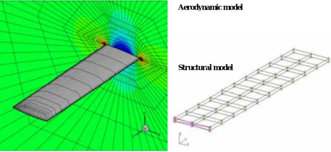
curvilinear body-fitted meshes. The structural discretization uses a finite-element model, analyzed with MSC.Nastran. The coupling approach used is described in Woodgate et al. (2005). For the Goland wing we consider throughout this section the coarse aerodynamic grid, and structural model are depicted in Figure 1.
In order to estimate the stability properties of the aeroelastic system, we could integrate the discrete system forward in time for each parameter-set and condition of interest - but this is computationally expensive. Instead we perform a linear stability analysis of the coupled discrete system (Marques et al., 2010) about a stationary solution. This involves a linearization of the full non-linear coupled solver, resulting in a Jacobian matrix containing both fluid, structure and cross-terms. Finding the eigenvalues of this matrix directly is intractable - therefore the system is factored using the Schur complement, resulting in a non-linear eigenvalue problem with of the size of the number of structural parameters. By parameterizing the structure using the leading-order mode-shapes only, this number is kept small and the eigenvalue problem is solved rapidly with a Newton iteration. A typical result (for the Goland wing) is shown in Figure 2 (left). Eigenvalues associated with the first 4 structural modes are plotted, and it can be seen that at a certain altitude two modes interact, leading to one mode going unstable (real-part of eigenvalue greater than zero). To get a rough estimate of the influence of discretization error in the fluid the calculation is repeated on a much finer fluid mesh. The altitude at which flutter occurs is only very slightly changed.
Probabilistic collocation for uncertainty propagation
Now we consider the case in which the wing structure is imperfectly known. Consulting with aero-structure experts, a preliminary best-guess of ±5% variability in any given structural model parameter was made. In a precursory sensitivity analysis with linear aerodynamics, of the 31 structural parameters in the model, only 7 were identified as having a substantial influence on flutter. These 7 are treated stochastically (as uniform distributions) in the following, and the influence of the remaining parameters is neglected.
Probabilistic collocation (PC), see e.g. Loeven (2010), is a means of computing statistics of the output of a computational model, given pdfs on the model's input parameters. The method uses a polynomial expansion based on Lagrange polynomials to approximate the response of the model in the uncertain parameter space.
Gaussian quadrature weighted by the pdf of the uncertain input is applied to compute the mean, variance, and higher moments of the output. By choosing the support points and Gauss rule appropriately, it is possible to achieve decoupling of the equations for different parameter values (collocation), and a higher-order approximation of the mean and variance of the output (spectral convergence). Multidimensional rules are build via tensor products of 1d rules - with cost exponential in the dimension. By Monte-Carlo sampling the polynomial response, approximate pdfs of output quantities can also be rapidly obtained.
Figure 1: Goland wing with coarse aerodynamic grid (left); eigenvalues of four dominant aeroelastic modes, for aerodynamics on fine and coarse grids (right).
Aerodynamic model
Structural model
We apply PC with a quadratic approximation in each of the 7 uncertain directions (i.e. PC(2)), requiring 37 = 2187 evaluations of the simulation code. This is feasible thanks to the low cost of the Schur-eigenvalue code.
The output for PC(2) is plotted in Figure 2 (right). The main subfigure shows the real part of the eigenvalue of the first aeroelastic mode (responsible for flutter), plotted as a function of altitude, as in Figure 2 (left). The multiple lines of varying thickness represent the uncertainty in this value caused by the specified structural uncertainty. The "truth" has a probability of 1/2 of lying to the right of the P = 1/2 line, a probability of 1/3 of lying to the right of the P = 1/3 line, etc. The histogram to the right approximates the pdf of the real eigenvalue at the red vertical line in the main subfigure (not the marginal pdf over altitude!). Similarly the histogram below approximate the pdf of the flutter altitude (i.e. the pdf of Re(λ) = 0), from which the probability of flutter can be quickly evaluated. Flutter is certain for an altitude < 6,000 ft, and guaranteed not to occur for an altitude >
14,000 ft, under the assumption that structural uncertainty is the dominant source. Clearly the predictive capability of the analysis is primarily limited by structural uncertainty and not discretization error. The conclusion that (under the relatively mild uncertainties on the structure) it is not possible to state the flutter altitude within 8000 ft is dismaying - this result is so broad as to be useless. Further this will remain true no matter how good the numerical code, and can only be reduced by experimental measurements of the structure, or some other aspect of the system.
Bayesian updating of structural uncertainty
Flight tests are one source of information commonly used to determine flutter altitude. Let us assume that an experiment has been performed using a Goland wing, and eigenvalues of the system at pre-flutter conditions are measured with a certain accuracy σd. Measurements at- or beyond flutter conditions are to be avoided lest the model be damaged (or the aircraft in a real flight-test). No experimental eigenvalue data currently exists for the Goland wing test-case, therefore to demonstrate the method artificial data is generated using simulation with added noise (a ``twin problem'' in the terminology of inverse problems).
Updating parameters in the presence of measurement data is known variously as model parameter estimation, model calibration, and system identification, and is accomplished in a stochastic setting using Bayes' theorem.
Two good introductory books on the subject are Tarantola (2004) and Gelman et al. (2004). The first step is to Figure 2: Eigenvalues of four dominant aeroelastic modes, for aerodynamics on fine and coarse grids (left);
uncertainty in single unstable eigenvalue due to structural uncertainty (right). The lower pdf displays the probability of flutter boundary occurring at a given altitude.
Discretization error Parametric uncertainty
define a prior: a probability distribution on the structural parameters encoding all information which is known about the parameters prior to observing the data, with pdf ρ0(α).
The second step is to describe the relationship between the model and the data, this is the statistical model. Let the vector of observed quantities be denoted d (the data). Let H(w, α) be an observation operator, which takes a model state w and parameter vector α, and returns the model's approximation of the observed quantities d. The model state w(α) satisfies the model equation:
! !,! = 0.
Under the assumptions: (i) that the noise in the measurements d is known and described by the random variable ε, and (ii) that there is no modeling error (for the correct choice of α), then the model and data are related as:
!=! !,! + ! s.t. ! !,! =0.
Given which the probability of observing data d given parameters α (the likelihood) is
! !! ∶= !! !−! !,! ,
where ρε(.) is the pdf of ε. For a prior and a likelihood, Bayes' theorem gives an explicit expression for the posterior, the probability of parameters given the observed data:
! !! ∝ ! !! !! ! ,
where the constant of proportionality (independent of α) is not usually of interest. In the Bayesian framework this posterior is regarded as the answer to the question: What is known about α?, and is therefore the updated estimate of the parameters. If we require a deterministic estimate of α - rather than the probabilistic posterior - then a reasonable choice is the most-likely value of α, the maximum a posteriori estimate (MAP estimate):
!!"#∶= argmax
! ! !! . Reducing uncertainty for the Goland wing
The procedure of the previous subsection is applied to the Goland wing test-case. We assume measurement data at 5 different accuracies, and at 5 distances from the "true" flutter point. This is intended to simulate flight-tests with differing measurement capabilities, and that are allowed only to approach flutter at different distances. In each case only a single complex eigenvalue is measured. In reality more data would be available, though we can only exploit that data which our model predicts. Once updated distributions on the structural parameters are estimated, those distributions can be propagated through the Schur-eigenvalue code to obtain updated (and hopefully narrower) distributions on the flutter altitude.
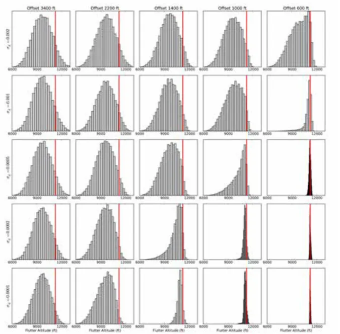
The posterior distributions on flutter altitude for calibrations using each of the 25 pieces of data are plotted in Figure 3. The prior is the same ±5% uniform distributions on each parameter used in the UQ study.
Immediately clear is that, in many cases, the level of uncertainty in flutter is reduced over the level present in the pure UQ study summarized in Figure 2 (right). Furthermore as the accuracy of the measurements increases, and the proximity to the flutter point decreases, more specific information about the true flutter altitude is identified. This is expected, but this study gives us quantitative information on how much we know about the flutter altitude given the data. For example at σd = 0.002 and a distance from flutter of 3400 ft, the posterior distribution looks almost identical to the prior, with a likely range of flutter altitude between 6000 and 13000 ft, indicating that data of that quality says very little about flutter. At the other extreme, with an accuracy of σd = 0.0001 and a distance from flutter of 600 ft, the true flutter altitude is identified in a very narrow band of less than 150 ft.
However in all cases, given the high-dimensional input parameter space (the 7 structural parameters) and the small quantity of added data (a single complex number), true values of individual structural parameters are only broadly identified. Nevertheless, thanks to the fact that the stability eigenvalue data is closely related to the
quantity of interest (the flutter altitude), the latter can be identified narrowly by the procedure, and the large uncertainty present in the original analysis is substantially reduced.
Figure 3: Dependence of posterior pdf of flutter altitude on distance of eigenvalue measurement from the flutter point (decreasing left-to-right), and accuracy of the measurement (increasing top-to-bottom).
Vertical red line is the "truth".
2. Kriging Regression of PIV Data using a Local Error Estimate
2Postprocessing Particle-Image Velocimetry (PIV) data is a challenging task. We introduce a method based on a interpolation method with origins in Bayesian statistics. Thanks to its stochastic heritage Kriging is able to incorporate estimates of noise in the data, and beliefs about the smoothness of the response. We apply Kriging to two purposes: interpolation of low-resolution data (from multiple planes), and improved estimates of velocity fields from poor quality images. In both cases Kriging is seen to provide substantial advantages over the best existing methods.
Gaussian Process Regression using Local Error Estimates
Usually, the post-processing of PIV data includes several steps, such as outlier detection, outlier replacement, smoothing, and in some cases interpolation to a finer grid. Each of these steps can involve different techniques, for example one might replace outliers by linear interpolation and increase the resolution with cubic spline interpolation. The Kriging predictor enables a different approach, it can provide a single-step prediction of the flow field at any (existing or new) set of grid-points and generally acts as a regressor - although in most cases the Kriging predictor is set to act as an exact interpolator.
Given the data !!"#=(!!"#,!!"#), the Kriging predictor for the flow field ! is given by (Wikle and Berliner, 2007):
! ! !!"# =!+!!! !+!"!! !! !!"#−!" , (2.1)
where the observation matrix ! selects the PIV data locations !!"#= !" from the complete set of locations !. For large domains we can reduce the computational cost by generating a sparse covariance matrix !, through approximation of the commenly used Gaussian covariance function with a spline.
The mean ! and variance !! of the flow are estimated from the statistical mean and standard deviation of the PIV data. The correlation range can be found from a Maximum Likelihood Estimate (Mardia et al., 1989) optimization, however in the following we use a Frequency-domain Sample Variogram optimization to reduce computational cost (de Baar et al., 2011; de Baar et al., 2012). In (2.1) usually !=0, such that Kriging is an exact interpolator, although a small ! = !" might be implemented for reasons of numerical stability, with ! of the order of the square-root of machine precision.
From a Bayesian perspective, we can introduce some amount of regression by choosing (Wikle and Berliner, 2007):
! = !!!!,
where !! is an estimate of the observation error, which is assumed to be globally constant, and ! is the error matrix. This can be interpreted as smoothing of the data, however from the Bayesian perspective the objective is not to smooth the data but to arrive at the most optimal prediction of the true flow. For Kriging with global error prediction presented here (Kriging GE), we use 32-fold random cross validation to estimate which value of !!
gives an optimal interpolation (Witten et al., 2011).
However in many cases we have an estimate of the velocity error per interrogation window (i.e. local). The same Bayesian perspective allows us to choose (Wikle and Berliner, 2007):
! = diag !!! ,
where we now interpret !! as a vector of local observation errors. Substituting this expression for ! into (2.1) results in a Kriging predictor with local error estimate (Kriging LE).
2From: J.H.S. de Baar, M. Percin, R.P. Dwight, B.W. van Oudheusden, H. Bijl, "Kriging regression of PIV data using a local error estimate", Experiments in Fluids (in preparation).
The question remains how to estimate the local observation error !!. This is a fundamental and long-standing problem in PIV, and a variety of rough estimates have been developed and are used, that are accurate to differing degrees depending on the source of the error. Ultimately, the user providing the PIV data might also quantify the accuracy of that data. Fortunately the Kriging predictor is fairly robust to inaccurate estimates of noise levels. In the we use the following simple model to estimate velocity error:
!! = !
!"!!− !"#!"#
where !"!! is the signal-to-noise ratio in the interrogation window !, and where the choice of !"#!"# results from the expertise of the PIV experimenter. We use 32-fold random cross-validation to estimate which value of
! gives the optimal interpolation.
Study of the Method for Synthetic Data
In this section we simulate PIV processing of synthetic images, interpolate the results to a finer grid using both conventional and new methods, and finally we perform a parametric investigation of the effect of bad seeding and reflections on the accuracy of the interpolation. This approach enables us to quantify the improved accuracy of an interpolation technique that employs a local error estimate of the PIV data. We consider the two dimensional incompressible flow (which we regard as "truth") given by:
!(!,!) = sin(2!") cos(2!"),
! !,! = −cos(2!") sin(2!"),
on the domain ! = [0,1] and ! = [0,1], which is visible on the right in Figure 4. From this flow we create synthetic image pairs with random seeding, Gaussian noise, reflection, 256x256 pixels, and 256 greyscale color- depth. A typical image is shown on the left in Figure 4.
We apply the Matlab PIV Toolbox MPIV (Mori, 2009) to reconstruct the flow field, using a recursive correlation algorithm with a final interrogation window size of 16x16 pixels and three point subpixel fitting.
Black arrows in Figure 4 show a typical reconstruction of the flow field. In this process we deliberately introduce several sources of error - such as noise, reflection, low image resolution, and low PIV data resolution - as a result of which we find a local offset of the PIV data with respect to the true flow, an example of which is visible in Figure 4. MPIV provides two different signal-to-noise ratio, of which we use the Peak-to-Mean ratio - that the ratio of the correlation peak height to the average correlation value in the fitting domain.
The next step is to interpolate the PIV data to a finer grid of 10! random grid-points. We compare the Root Mean Squared Error (RMSE) accuracy of three interpolation methods. For cubic spline interpolation the data is passed through the MPIV median filter, while both Kriging methods use the raw data directly. We perform a
Figure 4: Synthetic PIV image with seeding, noise, and reflection (left), reconstruction of the synthetic flow-field with PIV (right).
parametric study to quantify the effect of poor image quality on the accuracy of the interpolation. The first parameter we change is the seeding. Figure 5 (left) illustrates the effect of poor seeding on the RMSE accuracy of the three different interpolation methods. For underseeding we observe a dramatic increase of the cubic spline interpolation error. For Kriging GE this effect is less dramatic, while for Kriging LE we see only a very minor effect on the accuracy. This result is seen to be insensitive to the particular error estimate used.
The second parameter we increase is the intensity of the reflection. This leads to a region of poor image quality, resulting in a low SNR and therefore a high value of the local error estimate. This region of high estimated error roughly corresponds to the region where we observe a large offset of the PIV data with respect to the true flow.
The resulting interpolation accuracies are given in Figure 5 (right). Again, we see a dramatic increase of the cubic spline interpolation error, while the Kriging LE interpolation error remains much smaller. The reason for this is that in poor images the local offset is correlated with the local SNR. This relation is modeled by Kriging LE which results in an improved accuracy, as is illustrated by Figure 5 (right).
Application: Interpolation of Stereo PIV Data of the DelFly II MAV
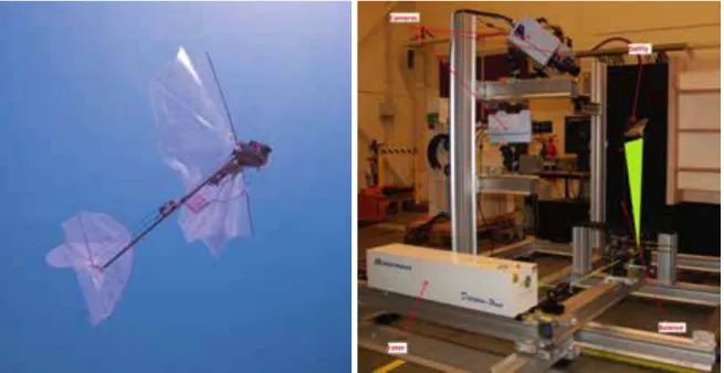
In this section, we implement the Kriging interpolation technique using local error estimate in the interpolation of the experimental data acquired via Stereoscopic Particle Image Velocimetry (Stereo-PIV) technique. The time-resolved PIV measurements were performed in the wake of the flapping-wing Micro Air Vehicle (MAV)
`DelFly' II (Figure 6 (left)) in forward flight configuration, the experimental setup is shown in Figure 6 (right).
Three-component velocity fields were obtained at several spanwise planes in the wake of the flapping wings and at a high framing rate to allow a reconstruction of the three-dimensional wake structure throughout the flapping cycle. The wake reconstruction was performed by interpolating between the measurement planes.
Experiments were performed for a large variety of parameters, i.e. flapping frequency, free-stream velocity, angle of attack and tail configuration. However, as the matter of interest is the performance of Kriging interpolation technique using local error estimate based on the Signal to Noise Ratio (SNR) of the PIV data, only some representative cases are represented and discussed in this paper. Before starting the discussion of the results, it is necessary to underline some important points regarding to interpretation of the results. First, it should be noted that only one half of the wake is visualized (the wake, however, is assumed to be nominally symmetrical) and that the region in the vicinity of the tail masked during PIV processing due to intensive reflection underneath and lack of illumination above the tail.
Results are shown in Figure 7, in which isocontours of the z-component of the vorticity are plotted. Accuracy of derivatives such as vorticity are naturally more sensitive to the quality of interpolation. Two prominent counter- rotating vortices are visible in Figure 7, corresponding to tip vortices from the upper and lower wing respectively. We compare the effectiveness of cubic-spline interpolation and Kriging GE (results for Kriging LE are currently being worked on, and are expected to be even better). There is no longer any "truth" velocity field, so the methods must be evaluated by reference to possible and plausible physical behaviour. In the cubic Figure 5: RMS error in predicted velocity field for three different interpolation techniques. As a function
of seeding density (left), as a function of reflection intensity (right).
spline reconstruction (top left), as well as the two main vortices we see a large quantity of spurious vorticity packets that are apparently non-physical and a result of (i) the large distance between measurement planes with respect to the in-plane resolution, (ii) the mismatch of fluctuations in the planes (which were measured at the same flapping phase but at different times), and (iii) the cubic spline not accounting for noise in the velocity vectors. In contrast in the Kriging interpolation (bottom left), the reconstruction is substantially smoother and spurious oscillations are reduced, such that we might examine the remaining vorticity blobs more closely, with a stronger belief that they may represent true flow features. The iso-plot (left) shows the complete flow domain.
By the robustness of its interpolation, and the ability to handle completely unstructured (point-cloud) data, error estimates, and derivative information natively, Kriging has provided a flexible means of analyzing the DelFly II data set that was possible only in a limited fashion before.
Figure 7: Vorticity fields. Top left: cubic spline interpolation, plan view. Bottom left: Kriging GE interpolation. Right: Kriging GE interpolation, perspective view with example velocity plane.
Figure 6: DelFly II in flight (left), the stereo PIV setup, open-jet nozzle visible on the extreme right (right).
3. Navier-Stokes Simulation in Gappy PIV Data
3PIV measurements are often affected by gaps, i.e. regions where no information regarding the velocity field is obtained. The gaps occur in areas where the particle image displacement cannot be evaluated. There are a wide variety of reasons for this: 1) absence of seeding particles due to inhomogeneous tracer dispersion or due to the centrifugal forces acting in vortices and wakes of high-speed flows (Schrijer and Walpot, 2010, Bitter et al., 2010); in this case the gaps occur irregularly in space and time; 2) laser light reflections from the surface of objects, which lead to corrupted tracer particle images; 3) shadows due to the presence of objects in the light path; 4) inaccessible regions for the imaging system.
The treatment of gaps in PIV data has received little attention. Generally considered as a byproduct of the vector validation problem, (detection and replacement of false vectors, see Westerweel, 1994 for instance) several data refill procedures have been proposed by practitioners. In essence, data refill procedures are nothing more than spatial interpolation or regression of neighbouring vectors. Several choices for the basis function are proposed, the lowest-order being bilinear interpolation of the known values at the boundary of the gaps. Gunes and Rist (2008) proposed to employ the Kriging method for stereoscopic data reconstruction. Ventura and Karniadakis (2004) investigated the possibility of using proper orthogonal decomposition (POD) for reconstructing flow fields from gappy data. The aforementioned methods can only reconstruct a monotonic velocity field or at most a field with a single peak inside the gap (a half wave).
The main idea behind the present method is to use the full governing equations of the flow to predict the velocity distribution inside the gap, in order to reduce the error associated with the data refill procedure. We employ a numerical solution of the 2d incompressible Navier-Stokes equations to estimate the velocity field within the gap, using a staggered-grid finite volume solver, with time-varying Dirichlet boundary conditions imposed using the velocity provided by the PIV data. Unusually for data assimilation problems the PDE is well-posed with these boundary conditions; in particular, boundary conditions on the pressure are not required.
Therefore assuming complete knowledge of BCs and belief in high accuracy of the experimental data, no stochastic approach is necessary - and we proceed deterministically with a standard NS solve. The initial condition on the velocity in the gap is unknown, but has a diminishing effect on the solution over time provided that information is convected out of the gap; therefore it is sufficient to specify any initial condition consistent with the boundary conditions at time zero, and integrate sufficiently far forward in time.
Numerical solution method
Considering a measurement domain with a gap Ω where no velocity is measured, the velocity field in Ωis computed by solving the unsteady Navier-Stokes equations, which in non-dimensional form read:
Conservation of mass:
∇
⋅V =0; (3.1)Conservation of momentum: p
t
∂ + =
∂
V
∇
R, (3.2)where the following units are chosen: velocity: Vref; length: L; density ρref, pressure: ρrefVref2. The vector R = [Ru Rv]T contains the contributions of advection and diffusion and is given by:
(
T)
1 Re
⎡ ⎤
= ⋅ − ⊗⎢⎣ + + ⎥⎦
R
∇
V V∇
V∇
V , (3.3)with Re = ρrefVrefL/µ the Reynolds number, and µ the coefficient of dynamic viscosity. To solve the Navier- Stokes equations in Ω, a finite volume method is employed using a Cartesian staggered grid (Welch et al., 1966). Following the approach by Veldman (1990), the continuity and momentum equations are combined to reformulate the problem as a Poisson equation for pressure, which in the discrete form reads:
3From: A. Sciacchitano, R.P. Dwight, F. Scarano, "Navier-Stokes Simulations in Gappy PIV Data", Experiments in Fluids, DOI:
10.1007/s00348-012-1366-5.
n 1 n n n+1
h h h h h h h
1 1
D G p D D
t t
Ω Ω Ω
δ δ
+ = ⎛⎜⎝ V +R ⎞⎟⎠+ ∂ V , (3.4)
where h represents the mesh spacing,
D
hΩ andD
h∂Ω are the discrete divergence operators at the points of the volume mesh and boundary mesh respectively, Gh is the discrete gradient operator, δt is the temporal step and n indexes the time level. Finally Vh, p and Rh are discrete quantities corresponding to V, p and R. Employing a central discretization for both convective and diffusive terms, equation (3.4) written out in full reads:n 1 n 1 n 1 n 1 n 1 n 1 n n n n
i 1, j i , j i 1, j i , j 1 i , j i , j 1 i 1 / 2 , j i 1 / 2 , j i , j 1 / 2 i , j 1 / 2
2 2
x y x y
n n n n
i 1 / 2 , j i 1 / 2 , j i , j 1 / 2 i , j 1 / 2
x y
p 2 p p p 2 p p 1 u u v v
h h t h h
Ru Ru Rv Rv
h h
δ
+ + + + + +
+ − + − + − + −
+ − + −
⎛ ⎞
− + − + − −
+ = ⎜⎜⎝ + ⎟⎟⎠+
− −
+ +
, (3.5)
with i and j representing the position of a generic cell inside the domain and u and v the horizontal and vertical velocity components respectively. Finally the update is made via:
n+1 n n n 1
h
=
h+ δ t
h− δ tG p
h +V V R
, (3.6)The pressure values computed from equation (3.5) guarantee that the velocity components obtained by solving (3.6) satisfy the incompressibility constraint (3.1).
Critically for this approach, (3.4) and (3.6) can be solved imposing boundary conditions only on the velocity and not on the pressure (Ferziger and Peric, 2002). The boundary conditions on V are provided at discrete time instants by the PIV measurements and are imposed as Dirichlet conditions. In order for the numerical scheme to be stable, the spacing h of the computational mesh and the time step δt are selected according to the conditions proposed by Ferziger and Peric (2002) for the linear convection-diffusion equation. To fulfill those conditions, δt often needs to be smaller than the time interval Δt between PIV recordings. Therefore, the velocity boundary conditions at intermediate time instants are computed through interpolation in time of the PIV velocity data.
The time interpolation for the boundary conditions is based on the advection model proposed by Scarano and Moore (2011).
Application: Treatment of Shadow Regions
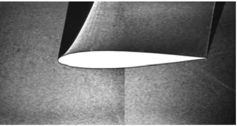
The technique is applied to an experiment in air of a rod-airfoil configuration. A cylindrical rod of 6 mm diameter is mounted 10.2 cm upstream of a NACA 0012 airfoil, having a chord of 10 cm and placed at zero angle of attack. The airfoil is made out of Plexiglas in order to be transparent to the laser light. The nominal free-stream velocity is set to 15 m/s, yielding Reynolds numbers of 6,000 and 100,000 with respect to the rod diameter and the airfoil chord respectively. The temporal separation between laser pulses is 50 µs, while the acquisition frequency is 2,700 Hz. The field of view size is 164×83 mm, imaged by 1939×1024 pixels. A thorough description of the experiment is reported in Lorenzoni et al., 2009.
The illumination is directed from the bottom of the field of view upwards, tilted clockwise by 11 degrees.
According to Snell’s law (Born and Wolf, 1999), when a light ray passes from air (refractive index n1 = 1.000) to Plexiglas (refractive index n2 = 1.488), it undergoes a deflection that depends on the angle between the incident ray and the normal to the interface. The deflection is negligible in the central part of the airfoil, where the incident and refracted rays are roughly parallel to the normal to the interface. In contrast, where the airfoil curvature is larger, i.e. at the leading and trailing edges, the refraction becomes so strong that non-illuminated regions are generated above the airfoil, see Figure 8.
For both the shadow regions A and B, above the leading and the trailing edge respectively, the numerical simulation is conducted in rectangular domains, indicated by the dashed lines in Figure 9. The first region, ΩA is composed by 112×88 cells, corresponding to 56×44 PIV grid nodes, while ΩB is composed by 62×100 cells, which correspond to 31×50 PIV grid nodes. The region containing measurement data inside the numerical domains serves as the buffer region B. Both numerical domains ΩA and ΩB exhibit a central region where no
PIV data is present and two lateral regions where particle image velocimetry vectors have been measured; the numerical solution is calculated in the entirety of the rectangular domains, but it is retained only in the central regions. At the unknown boundaries, the boundary conditions are computed as a linear interpolation of the measured PIV velocity data. Figure 9 shows an example of reconstructed instantaneous velocity fields. In both the shadow regions, the velocity components computed with the Navier-Stokes solver exhibit good agreement with the surrounding experimental data.
Figure 9: Instantaneous reconstructed velocity fields. Left: horizontal velocity component; right: vertical velocity component.
The added value of the present technique with respect to interpolation approaches is evident when small flow structures need to be reconstructed in the shadow region. In Figure 10, the motion of two vortices a and b is illustrated. At time t = 0, vortex a has a single core while vortex b has two distinct cores; both the vortices are on the left of the shadow region. The two vortices are adverted downstream by the flow and pass through the shadow region, where the velocity is calculated via the numerical simulation. The proposed filling approach allows tracking the vortices within the shadow region and estimating the distance between them within 5%
accuracy. However, modulation effects are noticed which have two main consequences: reducing the peak vorticity up to 50% of the original value and merging the two cores of vortex b in a single-core vortex (see Figure 10). Downstream of the shadow region, the vorticity is measured from PIV data: the peak vorticity is recovered and the two cores of vortex b become distinct again.
Figure 8: Double-frame recording of particle images on a transparent NACA 0012 airfoil (laser light directed from below) in the wake of a rod (outside the field of view).
Figure 9: Instantaneous reconstructed velocity fields. Left: horizontal velocity component; right: vertical velocity component.
Figure 10: Vorticity contours showing the convection of two vortices a and b through the shadow region.
Left: reconstruction through the Navier-Stokes solver; right: reconstruction through a bicubic interpolation of the velocity boundary values.
t = 0.74 ms
t = 1.48 ms
t = 2.22 ms
t = 2.96 ms
t = 3.70 ms a b
a b
a b
a b
a b
a b
a
a b
a b b?
a? b?
Navier-Stokes simulation in the gap Bicubic interpolation
Conclusions and Further Work
In all engineering tasks use is made of both experimental data and simulation. We have shown how these may be combined in a variety of situations with Bayesian inference, assisted with appropriate numerical algorithms, to give results that are more complete and/or accurate than either simulation or experiment alone. The existence of Bayes as a unifying framework allows sharing of methods and implementations across widely varying application domains. We are firm believers in the use of Bayesian statistics for exploiting modern high-fidelity CFD solvers and rich data provided by modern experimental methods.
In each of the applications discussed work is ongoing, in order:
1. The main limitation of the current study was the use of manufactured data, which allowed us to assume that model inadequacy was negligible, and gave us exact knowledge of the experimental noise. Next steps are application to aeroelastic wind-tunnel tests, where a more complete statistical model will be necessary.
2. There are a number of directions in which Kriging PIV interpolation can be developed. Algorithms used to identify window displacements in PIV are usually iterative, with an initial low-quality velocity field being used to inform window distortion in a second step. Kriging is ideal for reconstructing this initial velocity field from noisy velocity vectors, and could help improve the efficiency and stability of these algorithms. We would also like to incorporate physical information into the interpolation via the covariance structure - this will allow the imposition of known properties like zero divergence or conservation, and improve the quality of results with bigger gaps (Dwight, 2010).
3. The gappy PIV technique relies on velocities being measured at all boundaries of a gap - which is an unusual situation, not even satisfied by our rod-aerofoil test-case. Compensating with interpolation at the boundary will not always be feasible, or give acceptable results. Similarly the velocity data must be accurate everywhere on the boundary. The method also relies on the assumption of incompressibility, without which velocity-only BCs lead to an ill-posed problem. Even worse if we desire to increase time resolution with this method, there is no way to match the numerical solution to measured data after a given time. All these issues can be resolved by also treating this problem stochastically. In this case a non-linear Kalman filter is an appropriate stochastic method, which may be derived from Bayesian statistics, Wickle and Berliner (2007). We are investigating the Ensemble Kalman Filter (EnKF) and Ensemble Optimal Interpolation (EnOI), Evensen (2003). Uncertainities in ICs, BCs and the model will be reflected in the solution.
References
[1] de Baar, J.H.S., Dwight, R.P. and Bijl, H. (2011). Fast maximum likelihood estimate of the Kriging correlation range in the frequency domain. In IAMG Conference Salzburg.
[2] de Baar, J.H.S., Dwight, R.P. and Bijl, H. (2012). Speeding up kriging: fast estimation of Kriging hyperparameters in the frequency-domain. To be submitted.
[3] de Baar, J.H.S, Percin, M., Dwight, R.P., van Oudheusden, B.W. and Bijl, H. (2012). Kriging regression of PIV data using a local error estimate. Experiments in Fluids (in preparation).
[4] Bitter, M., Scharnowski, S., Hain, R. and Kaehler, C.J. (2010). High-repetition rate PIV investigations on a generic rocket model in sub- and supersonic flows. Exp. Fluids 50:1019-30.
[5] Born, M. and Wolf, E. (1999). Principles of optics. Cambridge university press, Cambridge, U.K.
[6] Dwight, R.P. (2010). Bayesian inference for data assimilation using Least-Squares Finite Element methods. IOP Series: Materials Science and Engineering, Vol. 10 (1), pp. 222-232, doi:10.1088/1757- 899X/10/1/012224, 2010.
[7] Dwight, R.P., Haddad-Khodaparast, H. and Mottershead, J.E. (2012). Identifying Structural Variability using Bayesian Inference. Proc. Uncertainty in Structural Dynamics (ISMA/USD).
[8] Dwight, R.P., Marques, S., Bijl, H. and Badcock, K.J. (2011). Reducing Uncertainty in Aeroelastic Flutter Boundaries using Experimental Data. International Forum on Aeroelasticity and Structural Dynamics, Paris, IFASD-2011-71.
[9] Evensen, G. (2003). The Ensemble Kalman Filter: Theoretical formulation and practical implementation. Ocean Dynamics 53(4), pp. 343-367.
[10] Ferziger, J.H. and Peric, M. (2002). Computational methods for fluid dynamics. Springer.
[11] Gelman, A., Carlin, J.B., Stern, H.S., and Rubin, D.B. (2004). Bayesian Data Analysis. CRC Press.
[12] Gunes, H. and Rist, U. (2008). On the use of kriging for enhanced data reconstruction in a separated transitional flat-plate boundary layer. Physics of Fluids 20, 104109.
[13] Kennedy, M. and O’Hagan, A. (2001). Bayesian calibration of computer models (with discussion). Journal of the Royal Statistical Society, Series B., 63, 425–464.
[14] Khalil, M., Sarkar, A., and Poirel, D. (2010). Application of Bayesian inference to the flutter margin method: New developments. ASME Conference Proceedings, 2010(54518), 1143–1151.
doi:10.1115/FEDSM- ICNMM2010-30041.
[15] Lind, R. and Brenner, M. (1997). Robust flutter margins of an F/A-18 aircraft from aeroelastic flight data. Journal of Guidance, Control and Dynamics, 20(3), 597–604.
[16] Loeven, G. (2010). Efficient Uncertainty Quantification in Computational Fluid Dynamics. Ph.D. thesis, TU Delft, Department of Aerodynamics.
[17] Lorenzoni, V., Tuinstra, M., Moore, P.D. and Scarano, F. (2009). Aeroacoustic analysis of a rod-airfoil flow by means of time-resolved PIV. 15th AIAA/CEAS Aeroacoustic Conference (30th AIAA Aeroacoustic Conference), Miami, Florida, May 11-13.
[18] Mardia, K.V. and Marshall, R.J. (1984). Maximum likelihood estimation of models for residual covariance in spatial regression. Biometrika, vol. 71, no. 1, pp. 135–146.
[19] Marques, S., Badcock, K., Khodaparast, H., et al. (2010). Transonic aeroelastic stability predictions under the influence of structural variability. Journal of Aircraft, 47(4), 1229–1239.
[20] Mori, N. (2009). MPIV. http://www.oceanwave.jp/softwares/mpiv.
[21] Pettit, C. L. and Beran, P. S. (2006). Spectral and multiresolution wiener expansions of oscillatory stochastic processes. Journal of Sound and Vibration, 294(4–5), 752–779.
[22] Scarano, F. and Moore, P.D. (2011). An advection-based model to increase the temporal resolution of PIV time series. Exp Fluids, DOI 10.1007/s00348-011-1158-3.
[23] Schrijer, F.F.J. and Walpot, L.M.G.F.M. (2010). Experimental investigation of the supersonic wake of a reentry capsule. Proc. AIAA 2010-1251, 48th AIAA Aerospace Sciences Meeting (Orlando, FL).
[24] Sciacchitano, A., Dwight, R.P. and Scarano, F. (2012). Navier-Stokes Simulations in Gappy PIV Data. Experiments in Fluids, DOI: 10.1007/s00348
[25] Tarantola, A. (2004). Inverse Problem Theory and Methods for Model Parameter Estimation. Society for Industrial and Applied Mathematics.
[27] Venturi, D. and Karniadakis, G.E.M. (2004). Gappy data and reconstruction procedures for flow past a cylinder. J. Fluid Mech. vol. 509 pp. 315-336.
[28] Welch, J.E., Harlow, F.H., Shannon, J.P. and Daly, B.J. (1966). The MAC method, a computing technique for solving viscous incompressible, transient fluid-flow problems involving free surfaces. Report LA-3425, Los Alamos Research Laboratories, Los Alamos, NM.
[29] Westerweeel, J. (1994). Efficient detection of spurious vectors in particle image velocimetry data. Exp.
Fluids 16:236-247.
[30] Wikle, C.K. and Berliner, L.M. (2007). A Bayesian tutorial for data assimilation. Physica D:
Nonlinear Phenomena, vol. 230, no. 1-2, pp. 1–16.
[31] Witten, I.H., Frank, E. and Hall, M. (2011). Data Mining: Practical Machine Learning Tools and Techniques. 3rd Edition. Morgan Kaufmann.
[32] Witteveen, J., Sarkar, S., and Bijl, H. (2007). Modeling physical uncertainties in dynamic stall induced fluid- structure interaction of turbine blades using arbitrary polynomial chaos. Computers and Structures, 85, 866–878.
[33] Woodgate, M., Badcock, K., Rampurawala, A., et al. (2005). Aeroelastic calculations for the Hawk aircraft using the Euler equations. Journal of Aircraft, 42(4), 1005–1012.
[34] Xiu, D. and Karniadakis, G. (2002). The Wiener-Askey polynomial chaos for stochastic differential equations. SIAM J. Sci. Comput., 24(2), 619–644.
[35] Zimmerman, N. and Weissenburger, J. (1964). Prediction of flutter onset speed based on flight testing at subcritical speeds. Journal of Aircraft, 1(4), 190–202.