Purification for the Fastest Bootstrap of a Quantum Link

(1)

Bachelor Thesis 2017

Optimized Fidelity Estimation in

Purification for the Fastest Bootstrap of a Quantum Link

迅速な量子リンク作成のための純粋化におけるフィデリティ推定の最適化

Keio University, Faculty of Environment and Information Studies Takafumi Oka

(2)

Abstract of Bachelor’s Thesis

Academic Year 2017

Optimized Fidelity Estimation in Purification for the Fastest Bootstrap of a Quantum Link

Quantum networking has increasingly become significant for a variety of its applications such as quantum key distribution (QKD). In quantum networking reliablity of a connection depends on the quality of Bell pairs (a type of quantum state) used. When the fidelity is not suﬃciently high, we need to conduct purification to increase the fidelity. However, determining the quality of a given Bell pair is by no means a trivial process. Nevertheless, literature established on quantum networking often presupposes the knowledge of the fidelity of the state in question without reference to actual means of state analysis. While existing quantum state tomography methods proposed in e.g.

[1] could achieve the purpose, they are not designed to function in synchronization with nodes involved in the link, being redundant and ineﬃcient when employed for operational link creation in quantum networking, and thus far from optimal for our purpose.

The thesis will present an optimized configuration of state analysis and purification, tailored for our very situation, with a view toward the quickest possible link creation.

Simulation of physical equipment, state analysis, and evaluation of the proposal are implemented in Python.

Keywords :

1. Quantum networking, 2. Quantum computing, 3. Quantum state tomography,

Keio University, Faculty of Environment and Information Studies

Takafumi Oka

(3)

List of Figures

2.1 Representation of a qubit on the Bloch sphere: every 1-qubit state can be drawn as a point on the surface of the sphere, providing visually perceptible representation. . . . 7 2.2 List of diagram symbols for X, Y, Z, Hadamard, and CNOT gates: these

will be frequently used throughout the thesis. . . . . 10 2.3 Symbol for the measurement operator in Z axis (the left symbol stands

for the right one unless otherwise noted), corresponding to the measurement by the operatorsM₀ and M₁ (in the notation of 2.2.1). . . . 10 2.4 Symbol for the measurement operator in X axis, corresponding to the

measurement by the operators M_|₀_⟩₊_|₁_⟩_/^√₂ and M_|₀_⟩−|₁_⟩_/^√₂. . . . 11 2.5 Symbol for the measurement operator in Y axis, corresponding to the

measurement by the operators M_{|0⟩+i|1⟩/}^√₂ and M_{|0⟩−i|1⟩/}^√₂. . . . 11 2.6 A Bell pair, with two photons entangled: measurements of one pho-

ton aﬀects measurements of the other. Local operations on one photon immediately aﬀecte the other at a distant location! . . . . 12 2.7 Circuit diagram of quantum teleporation: Bob applies his operation

depending on the measurement result at Alice. . . . 12 2.8 Circuit diagram of entanglement swapping . . . . 14 2.9 Entanglement swapping: initial state. Node 1 and 2 share one entangled

photon pairs, and Node 2 and 3 also share another entangled photon pair, with two photons in total at Node 2. . . . 14 2.10 Entanglement swapping: teleporting the state of one particle of Node 2

to Node 3 using the same procedure as quantum teleportation. . . . 15 2.11 Entanglement swapping: the particle at Node 1 is now entangled to the

particle at Node 3, resulting in a longer entanglement. . . . 15 2.12 Extended purification circuit: now capable of suppressing both bit flip

and phase flip errors. . . . 17 2.13 Multiple rounds of purification, increasing the fidelity still further after

each round. . . . 17 2.14 A scheme of two nodes sharing an entangled photon pair: the photon

1 and 2 constitute the entanglement, both having been emitted by the Entangle Photon Pair Sender in the middle. . . . 18 2.15 A quantum link with Node Controllers: the Controllers are in chrage of

making operational decisions such as choosing measurement bases and fidelity assessment of states, involving state estimation methods. . . . . 19

(6)

2.16 Fidelity and the process of state reconstruction in tomography: looking at the state from diﬀerent angles enables reconstruction of the state . . 20 2.17 Measurement bases and their respective points on the Bloch sphere:

measurements with respect to these bases “project” a given state to their respective points on the sphere probabilistically. . . . 21 2.18 State tomography for 1-qubit: the actual fidelity is between the ideal

state and the actual state (the latter of which cannot be seen) and the reconstruction fidelity is between the state reconstructed by the maxi- mum likelihood (see Section 2.5.1) and a set of states generated by the error estimation routine (see Section 2.5.2), representing accuracy of the reconstruction. . . . . 21 3.1 Flowchart at Node 1 in the distributed model: both Node 1 and 2 con-

duct tomography concurrently, exchanging each other’s reconstructed density matrices. . . . 26 3.2 Flowchart at Node 1 in the master-slave model: only Node 1 conducts

tomography and is responsible for chooseing measurement bases and state reconstruction. . . . 27 3.3 Flowchart at Node 2 in the master-slave model: Node 2 receives the

tomography result and follows the decision of Node 1 regarding whether to proceed for applications. . . . 27 3.4 Flowchart of the bootstrap procedure of a quantum link: the number

of purifications increases until leading to the state being of a suﬃcient fidelity. . . . 28 4.1 Software Architecture of the whole program: the modules are seperated

by their respective roles. . . . 30 5.1 Relationship between Actual Fidelity and Reconstruction Fidelity based

on actual experimental data provided by Kwiat et. al., with no purification conduted. . . . . 35 5.2 Relations between the actual fidelity and the number of purifications

with no gate errors: the fidelity smoothly approaches to 1. . . . 36 5.3 Relations between the actual fidelity and the number of purifications

with CNOT gate errors present: the fidelity stagnates between 0.8 and 0.9. . . . 37 5.4 Relations between the reconstruction fidelity and the number of purifi-

cations with no gate errors: the reconstruction fidelity increases as the actual fidelity increases . . . . 38 5.5 Relations between the reconstruction fidelity and the number of purifi-

cations with CNOT gate errors present: the reconstruction fidelity also fluctuates as the actual fidelity does. . . . . 39

(7)

List of Tables

1.1 Notations and Symbols . . . . 3 2.1 Correspondence between Alice’s measurement outcomes and Bob’s state

at the time Alice obtained each outcome . . . . 13 2.2 Possible combinations of the states Alice and Bob have when only bit flip

errors occur: when the first and last cases occur the round of purification is considered successful, while the second and third cases lead to failure of the round. . . . . 16

(8)

Chapter 1 Introduction

1.1 Background I: Importance of Quantum Infor- mation Technology

Quantum information technology is known for its great potential in realizing things that are not feasible in classical information technology. Quantum computing, for instance, features suprising algorithms such as Shor’s algorithm that enables computing factor- ization of a number to prime numbers in polynomial time [2]. Quantum networking also has a wide range of applications; one of the most practically beneficial is quan- tum key distribution, or QKD, which enables more secure key distribution compared to classical [3]. In fact, the so-called E91 protocol [4] of QKD utilizes entanglement (see Section 2.3.1). Another interesting application of quantum networking utilizes distributed quantum states such as Bell states or GHZ states to realize decision-making among multiple nodes with essentially fewer steps of communication [5]. Furthermore, algorithms and schemes that make use of distributed quantum computing are proposed (e.g. [6]). Quantum repeatersare nodes that hold distributed quantum states, that are capable of applying certain operations to the states, and that are responsible for main- taing consistency in conjunction with other nodes for the involved nodes to function as a whole (as explained in Chapter 2.)

1.2 Background II: Challenges in Quantum Infor- mation Technology

All of these applications have one vital requirement in common: delivery of and operation to entangled quantum states, with as small noises and loss to the states as possible. It should first be noted that precise operation to quantum states is pro- hibitively diﬃcult as opposed to operation to classical bits (some of the examples of an actual experiment are done in e.g. [7, 8], which tell how large the obstacles are). In addition, another diﬃculty appears in an attempt to assess how well such delivery and operation has been done. This is attributed to the property of quantum states that a quantum state initiates a probabilistic collapse when measured, unlike classical bits, thereby requiring a myriad of measurements to reconstruct a given state, resorting to

(9)

both analytical and statistical reconstruction processes (called quantum state tomog- raphy, which will be introduced in Chapter 2). In particular, for quantum networking, we need to manage delivery and operation of resources (i.e. entangled states) in a real-time fashion.

This research project is intended to serve as an aid to solve the latter of those two challenges.

1.3 Problem Definition

It is worthwhile to devise a new method of state estimation that is particularly tailored for our quantum networking purpose. In order for the proposed method to be “tailored”

it needs to meet the following two requirements: that it keeps consistency with other nodes’ estimations that run concurrently and that the state estimation finishes rapidly enough to be used for bootstrapping a network. The former problem has been dealt with in the workshop paper [9], which proposes a master-slave protocol that supports two nodes about to initiate a quantum communication, with full state tomography embedded as a state estimation method.

This thesis addresses the latter problem and aims to propose an optimized state estimation method that can substitute for full state tomography. The evaluation of the proposed method will be based on the amount of time that it takes for two nodes to become ready for proceeding to further applications (e.g. QKD). Because the most time-consuming step involved is repeated generation, transmission, and measurement of Bell states, shortening the amount of time requires fewer generations of Bell pairs, hence in turn demanding a state analysis method of suﬃcient accuracy with fewer measurement results.

Of course generation of Bell states, latency of transmission, and measurement eﬃ- ciency depend upon particular equipment, and assumptions have to be made to evaluate proposals.

1.4 Research Contribution

Upon completion of this research scholars will be able to adopt the proposed method for state analysis and to utilize quantitative data provided in the thesis to anticipate resource consumptions they need to allow for in an attempt to create a link. Fur- thermore, by combining the proposed protocol to support distributed state estimation, they will be able to sketch a model that they want to realize in reality, with the level of concreteness enough to calculate an amount of bootstrap time and latency caused during the course of bootstrap, provided the error rate in gates and Bell state initial fidelities (that depend on particular physical apparatus) are available. This set of information becomes particularly significant once applications former quantum networking (e.g. QKD) have been launched for practical use, where fidelity of the Bell pairs used dictate the applications’ proper function.

(10)

1.5 Thesis structure

Chapter 2 presents a concise introduction to quantum information technology with particular emphasis put on the knowledge of frequent use in this thesis. It is divided into five sections: Quantum States and Their Representations, Operations on Quan- tum States, Distributed Quantum States, Quantum Networking, and Quantum State Tomography. The Chapter is organized so as to move from local notions regarding quantum bits to global concepts used in conjunction with quantum states at distant locations.

Chapter 3 introduces the underpinning protocol that supports distributed state estimation.

Chapter 4 presents how the simulator used in this project works and how it is organized. It briefly lists the consisting modules and their respective roles, then picks major functions from each of the modules, with detailed explanation provided.

Chapter 5 presents the results obtained from the simulator. It first shows how state reconstruction looks like based on actual tomography and experimental data. Further, the relations between the number of purifications and the actual resultant fidelity are presented both in the case some errors are embraced and the case where there is no error.

Chapter 6 sums up the evaluation in Chapter 5, and yields conclusions that we have drawn from the research. Outlooks for future work will also be in Chapter 6.

1.6 Notations and Symbols

R The set of real numbers

C The set of complex numbers

Xⁿ The Cartesian product of n of X’s as sets

M_n(R)[M_n(C)] The set of n-by-n matrices whose entries are in R (or inC, respectively).

|ψ⟩] Arbitrary pure quantum state in Drac’s ket notation (|ψ⟩ ∈C²ⁿ for some n) ρ] Pure or mixed quantum state in density matrix form (ρ∈M₂ⁿ(C) for some n)

Table 1.1: Notations and Symbols

Notations and symbols used throughout the thesis are summarized in Table 1.1.

(11)

Chapter 2 Introduction to Quantum Information Technology

This chapter is a concise presentation of preliminary knowledge necessary to understand this research.

2.1 Quantum States and Their Representations

2.1.1 Quantum Bits

A quantum bit (henceforth qubit) is represented by a minimum unit of particles — atoms, electrons, or photons — to serve as the most fundamental computational unit in quantum information technology just as classical bits, each being 0 or 1 do, in classical computers. The essential diﬀerence of qubits lies in the fact that the particle involved can be in superposition: it holds two distinct states until measured, when it collapses into one of the two states probabilistically. We utilize this property of qubits for further applications.

One representation of a qubit is in the form of state vector, wherein the qubit |ψ⟩ is written as follows:

|ψ⟩=α|0⟩+β|1⟩ (2.1.1.1) where α and β are complex numbers satisfying |α|² +|β|² = 1 and |0⟩ and |1⟩ are defined to be the basis vectors

|0⟩ ≡ (1

0 )

, |1⟩ ≡ (0

1 )

More generally, when n qubits are available, n sets of each two distinct states in superposition form 2ⁿ possible combinations, represented by the equation

|ψ^′⟩=α0|00. . .0⟩+α1|00. . .1⟩+· · ·+α2ⁿ−1|11. . .1⟩ (2.1.1.3)

(12)

where each α_i is a complex number, ∑₂ⁿ₋₁

i=0 |α_i|² = 1 and |k₁k₂. . . k_n⟩(each k_i is either 0 or 1) is the standard unit vector whose m-th component is 1 and other components are 0 where m=∑n

i=02ⁱki, the decimal representation of the binary digitk1k2. . . kn. This | ⟩ notation is called Dirac’s ket notation [5]. For each |ψ⟩, ⟨ψ| is defined to be the transpose with complex conjugate taken for each entry: if

|ψ⟩=



 c₁

... c_n



, (2.1.1.4)

then ⟨ψ| is defined to be

⟨ψ|=(

c₁ · · · c_n)

. (2.1.1.5)

where c_i is the complex conjugate of c_i.

We define a few operations for state vectors in Dirac’s notation. Let

|ψ1⟩=



 a₁

... a_n



 (2.1.1.6)

and

|ψ₂⟩=



 b₁

... b_n



. (2.1.1.7)

Then the outer product of |ψ1⟩ and |ψ2⟩,|ψ1⟩ ⟨ψ2|, is defined to be [5]

|ψ₁⟩ ⟨ψ₂| ≡





a₁b₁ a₁b₂ · · · a₁b_n ... . .. · · · ... a_nb₁ a_nb₂ · · · a_nb_n



; (2.1.1.8)

the tensor product of |ψ₁⟩ and |ψ₂⟩ is

|ψ₁⟩ ⊗ |ψ₂⟩ ≡





 a₁b₁ a₁b₂ ... a₁b_n a2b1

... a₂b_n

... a_nb_n







; (2.1.1.9)

and theinner product of |ψ₁⟩ and |ψ₂⟩ is

⟨ψ₁|ψ₂⟩ ≡

∑n i=1

a_ib_i. (2.1.1.10)

(13)

As is done in usual linear algebra, it is possible to consider change of basisfor state vectors. In fact, the basis set |00⟩, |01⟩, |10⟩, and |11⟩ is called computational basis, one of the most frequently used basis set for 1-qubit states. Another basis set of as frequent use is called Bell basis, which consists of |Φ⁺⟩, |Φ⁻⟩, |Ψ⁺⟩, and |Ψ⁻⟩; for the formal definition of these four states, see Section 2.3.1.

2.1.2 Density Matrix

Adensity matrix is another representation of a quantum state. When a state is part of a larger system and cannot be described as a superposition of known pure states that lie inside the system, the state is said to bemixedand expressed as a linear sum of pure states that we do know lie within the system, with a classical probability multiplied to each pure state in the sum. Density matrices are used to represent such states. To make the formal definition, let{p_i}be the set of classical probabilities and let the state be a combination ∑

ip_i|ψ_i⟩. The density matrix representing this state is defined to be

ρ≡∑

i

p_i|ψ_i⟩ ⟨ψ_i|. (2.1.2.1) Note that, when there are n qubits, each |ψ_i⟩ is a 2ⁿ-dimensional complex vector and thus |ψ_i⟩ ⟨ψ_i| is a 2ⁿ×2ⁿ-complex matrix. In particular, when 1 is the only element in {p_i}, the ρ is just |ψ⟩ ⟨ψ| and represents nothing but a pure state. Because we do not know the whole system (which is ultimately the universe) that surrounds us and the state of interest, every quantum state we face in reality needs to be represented as a density matrix.

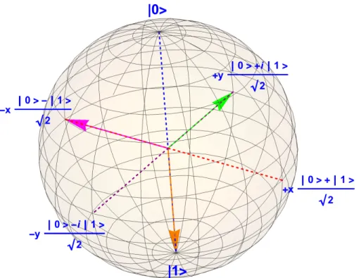
2.1.3 Bloch Sphere

2.1 A visually useful representation for 1-qubit states is the Bloch sphere. Let us represent the state |ψ⟩=α|0⟩+β|1⟩ in this sphere. Rewriting|ψ⟩ as

|ψ⟩=|α| |0⟩+ exp(−iθ)β|1⟩. (2.1.3.2) Using the identity|α|²+|β|² = 1, the equation above can be written as

|ψ⟩= cosφ₁+ exp(iφ₂) sinφ₁ (2.1.3.3) where cosφ₁ =|α|, φ₂ = arg(β)−θ, arg(β) is the angle at which β lies with respect to the x-axis in the complex plane. This one-to-one correspondence between 1-qubit state vectors and points on the surface of the unit sphere allows us to depict a given 1-qubit state on the sphere as in Figure 2.1.

(14)

Figure 2.1: Representation of a qubit on the Bloch sphere: every 1-qubit state can be drawn as a point on the surface of the sphere, providing visually perceptible representation.

2.1.4 Fidelity

We introduce one of the quantities of frequent use in further chapters. Fidelity is a quantity that derives from given two mixed states, ranging from 0 to 1, and represents

“similarity” between the states. More precisely, given density matrices ρ₁ and ρ₂, the fidelity between them is defined to be [1]

F(ρ₁, ρ₂)≡ {

Tr (√√

ρ₁ρ₂√ ρ₁

)}²

. (2.1.4.1)

2.2 Operations on Quantum States

2.2.1 Measurements

As mentioned in Section 2.1.1, qubits collapse into either 0 or 1 probabilistically. This collapse is invoked bymeasurement. An operation of measurement to a quantum state is, in mathematical terms, defined to be a linear transformation called ameasurement operator. We can thus regard each measurement operator as a matrix that transforms the state vector into another. We need to choose a measurement basis to conduct measurement. For 1-qubit measurement, we may choose any 1-qubit state vector for a

(15)

measurement basis, and the corresponding measurement operatorM_ψ is defined to be

M_ψ ≡ |ψ⟩ ⟨ψ| (2.2.1.1)

with the choice of basis |ψ⟩. The probability of measuring the outcome |ψ⟩ is then defined to be

p_ψ ≡ ⟨ψ|M_ψ^∗M_ψ|ψ⟩. (2.2.1.2) where M_ψ^∗ is defined to be the conjugate transpose of M_ψ. The preceding illustration of ”probabilistic collapse” of |ψ⟩ made in Section 2.1.1 is precisely the measurement operation with basis |0⟩ and |1⟩. In fact, following the definitions, the corresponding measurement operators become

M₀ =|0⟩ ⟨0|= (1 0

0 0 )

(2.2.1.3) and

M₁ =|1⟩ ⟨1|= (0 0

0 1 )

. (2.2.1.4)

In this setting, we measure 0 in probability ⟨0|M₀^∗M₀|0⟩ and 1 in ⟨0|M₀^∗M₀|0⟩. An easy calculation will show they are equal to |α|² and |β|², respectively.

Another important notion is orthogonality. Two state vectors |ψ⟩ and |φ⟩ are said to be orthogonal if the relation

⟨ψ|φ⟩= 0 (2.2.1.5)

holds. Consider an arbitrary 1-qubit state|ψ⟩=α|0⟩+β|1⟩. Since we have the identity

|α|² +|β|² = 1, the probability of measuring 0 for |ψ⟩ is the complementary event of measuring 1. In fact, for any orthonormalbasis {|v₁⟩,|v₂⟩}, which is, for any basis set whose elements are of norm 1 and orthogonal, we can write |ψ⟩=α^′|v₁⟩+β^′|v₂⟩ with some suitableα^′ ∈C and β^′ ∈C, and the relation

|α^′|²+|β^′|² = 1 (2.2.1.6) still holds, for any basis transformation between orthonomal bases preserves the norm.

More generally, for any n-qubit states, there always exist 2ⁿ vectors, v₀, . . . , v₂ⁿ₋₁ in C²ⁿ, such that any two of them are orthogonal and they are all of norm 1. For an n-qubit state |ψ⟩, the analogus relation

2∑ⁿ−1 i=0

|α_i|² = 1 (2.2.1.7)

holds where |ψ⟩= ∑2ⁿ−1

i=0 α_i|i⟩, where |i⟩ are the orthonormal basis for C²ⁿ. Because of the orthogonality, theoretically we need only 2ⁿ−1 probabilities to represent the state |ψ⟩. The notion of orthogonality will be necessary in Chapter 4.

(16)

2.2.2 Quantum Gates

In quantum computing we have an analogus notion for circuits in classical computing, quantum circuits, where a set of quantum states pass through quantum gates, being transformed by eﬀects of the gates, until they are finally measured to yield outcomes.

Given that state vectors are complex vectors of norm 1, complex matrices that preserve norms, namely unitary matrices¹, transform state vectors to state vectors.

Therefore it is natural to consider quantum gates that are unitary transformations.

The quantum gate of most frequent use throughout this research is Controlled- not gate, or CNOT gate. CNOT gate takes two qubits, the first qubit being called control qubit and the second target qubit. Let the control qubit and the target qubit be expressed as

|ψ₁⟩=α₁|0⟩+β₁|1⟩ (2.2.2.1) and

|ψ₂⟩=α₂|0⟩+β₂|1⟩, (2.2.2.2) respectively. Then the two qubit state is written as

|ψ⟩=|ψ1⟩ |ψ2⟩

=α₁α₂|00⟩+α₁β₂|01⟩+β₁α₂|10⟩+β₁β₂|11⟩.

The CNOT gate exchanges the two terms of first qubit 1 in |ψ⟩ each other:

α₁α₂|00⟩+α₁β₂|01⟩+β₁α₂|10⟩+β₁β₂|11⟩

−−−−→

CN OT α₁α₂|00⟩+α₁β₂|01⟩+β₁α₂|11⟩+β₁β₂|10⟩.

Recalling that the states above are vectors in C⁴ (see Section 2.1.1 in this Chapter), this operation is clearly a linear transformation ofC⁴ and thus written in matrix form as

CN OT =







1 0 0 0 0 1 0 0 0 0 0 1 0 0 1 0





. (2.2.2.3)

We will see in a subsequent section that this CNOT gate plays an essential role in a procedure called purification.

Hadamard gate is another gate for 1-qubit states that is used in quantum tele- portaion, and in turn, entanglement swapping, which will be formally introduced in Section 2.3.2 and 2.3.3, respectively. This gate takes |0⟩ to (|0⟩+|1⟩)/√

2, and |1⟩ to (|0⟩ − |1⟩)/√

2; in matrix form it is expressed as [5]

Hadamard= 1

√2

(1 1 1 −1

)

. (2.2.2.4)

Other 1-qubit gates of as frequent use areX gate,Y gate, andZ gate. These are defined as the following [5]:

1There are several equivalent definitions for unitary matrices, one of which is the one used here, to require the matrix preserve the norm of any vector being transformed.

(17)

X = (0 1

1 0 )

, (2.2.2.5)

Y =

(0 −i i 0

)

, (2.2.2.6)

and

Z =

(1 0 0 −1

)

. (2.2.2.7)

These basic gates have commonly used symbols for circuit diagrams as in Figure 2.2.

X

H Z Y

=

✓0 1 1 0

◆

=

✓0 i

i 0

◆

=

✓1 0

0 1

◆

= 1 p2

✓1 1

1 1

◆

= 0 BB

@

1 0 0 0 0 1 0 0 0 0 0 1 0 0 1 0

1 CC A

Figure 2.2: List of diagram symbols for X, Y, Z, Hadamard, and CNOT gates: these will be frequently used throughout the thesis.

In addition, measurement operators (with respect to Z, X, and Y axes) are also represented by similar symbols as illustrated in Figure 2.3, 2.4, and 2.5. These symbols will repeatedly appear in the rest of the thesis.

Z

=

Figure 2.3: Symbol for the measurement operator in Z axis (the left symbol stands for the right one unless otherwise noted), corresponding to the measurement by the operators M₀ and M₁ (in the notation of 2.2.1).

(18)

X

Figure 2.4: Symbol for the measurement operator in X axis, corresponding to the measurement by the operators M_|₀_⟩₊_|₁_⟩_/^√₂ and M_|₀_⟩−|₁_⟩_/^√₂.

Y

Figure 2.5: Symbol for the measurement operator in Y axis, corresponding to the measurement by the operators M_|₀_⟩_+i_|₁_⟩_/^√₂ and M_{|0⟩−i|1⟩/}^√₂.

2.3 Distributed Quantum States

2.3.1 Entanglement

Entanglement refers to a state of superpositon of more that one particle such that the outcome of measurement of one qubit is dependent on the outcome of the measurement of another qubit. For example, let

|ψ⟩= |00⟩√+|11⟩

2 . (2.3.1.1)

Observe that measuring 0 (or 1) for the first qubit immediately gives the knowledge of the outcome of the second qubit, 0 (or 1, respectively), without actually measuring the second one. This is an example of entanglement of quantum states.

One of the most frequently used type of entangled states in quantum networking is EPR pairs, or Bell pairs. They are 2-qubit states of one of the forms

Φ⁺⟩

= |00⟩√+|11⟩

2 , (2.3.1.2)

Φ⁻⟩

= |00⟩ − |√ 11⟩

2 , (2.3.1.3)

Ψ⁺⟩

= |01⟩√+|10⟩

2 , (2.3.1.4)

and Ψ⁻⟩

= |01⟩ − |√ 10⟩

2 . (2.3.1.5)

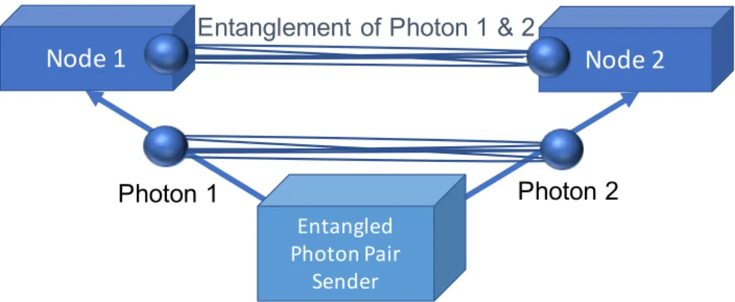
All these four are called Bell pairs. Figure 2.6 conceptually illustrates this.

(19)

| ⁺i = |00ip+ |11i 2

Figure 2.6: A Bell pair, with two photons entangled: measurements of one photon aﬀects measurements of the other. Local operations on one photon immediately aﬀecte the other at a distant location!

2.3.2 Quantum Teleportation

Quantum teleportation [10] exemplifies how entanglement can be practically useful.

Briefly speaking, a set of local operations² to an entangled state as well as to a given state|ψ⟩, enable “teleportation” of the state|ψ⟩. We explain how a qubit is teleported using an entangled state. The whole procedure of quantum teleportation is drawn in circuit form in Figure 2.7.

| i

₁

| ⁺i = |00i + |11i p2

2 3 2 3

1 2 3

H

XZ (No gate)

X Bob Z

Alice

Figure 2.7: Circuit diagram of quantum teleporation: Bob applies his operation depending on the measurement result at Alice.

Assume that Alice wants to teleport a qubit to Bob. Let |ψ⟩ = α|0⟩+β|1⟩ be the state that Alice wants to teleport and let the entangled state be the Bell pair³

|φ⁺⟩ = (|00⟩+|11⟩)/√

2 with the first qubit owned by Alice and the second by Bob;

thus Alice has two qubits and Bob has one. The whole state is expressed as

|ψ⟩Φ⁺⟩

= 1

√2 (

α|0⟩(|00⟩+|11⟩) +β|1⟩(|00⟩+|11⟩) )

. (2.3.2.1)

First Alice performs a CNOT gate, setting her qubit |ψ⟩as the controlling bit and the

2Operationhere means application of quantum gates to states andlocal operationsimply that the operations are made at the location where each of the qubits lies.

3The choice of a Bell pair among the four types is immaterial. It only aﬀects which type of gate Bob applies at the end of this procedure to complete the teleportation process.