A Comparative Study of the Viscosity of Ion Conducting Polymers based on the Bond Strength-Coordination Number Fluctuation Model and Other Models

A Comparative Study of the Viscosity of Ion Conducting Polymers based on the Bond Strength-Coordination Number Fluctuation Model and Other Models

SAHARA

, Masaru ANIYA

1

Department of Physics, Graduate School of Science and Technology, Kumamoto University, Kumamoto 860-8555, Japan

2

Department of Physics, Faculty of Science and Technology, State Islamic University (UIN) Alauddin, Makassar, Indonesia

Abstract

According to the Bond Strength-Coordination Number Fluctuation (BSCNF) model of the viscosity proposed some years ago by one of the authors, the viscosity is controlled by the relaxation of structural units that form the melt, and is described in terms of the average bond strength, coordination number and their fluctuations of the structural units. In the present paper, a comparative study of the viscosity of ion conducting polymeric system is presented. The analysis has been done though the BSCNF model and other models widely used in the literature such as Vogel-Fulcher-Tamman (VFT) and Williams-Landel-Ferry (WLF) equations. The result reveals that the three models describe well the temperature dependence of the viscosity reported experimentally. As a gross trend, the fragility of the polymeric system in consideration increases with the increase in the concentration of salts. Based on the analysis with the BSCNF model, such a behavior has been interpreted to arise from the disruption of the network that results by the addition of salts. The comparative study also reveals that the BSCNF model could provide a physical interpretation to the empirical parameters used in other models.

Keywords: Bond Strength-Coordination Number Fluctuation Model, Viscosity, Ion Conducting

Polymer, Vogel-Fulcher-Tamman Equation, Williams-Landel-Ferry Equation.

2 Introduction

Studies of physical properties of ion conducting polymeric materials are interesting from both, the academic and applied science points of views. These materials are characterized by their high ionic conductivity and high energy density power [1]. Potential applications of these materials in rechargeable lithium-ion batteries, electrochemical devices such as fuel cells, electrochromic displays, sensor, etc. have been investigated intensively [2,3]. Many studies have been also conducted in order to enhance the ionic conductivity and the mechanical stability of the materials [4]. However, fundamental understanding of the physical properties of the materials is not sufficient. For instance, previous study has indicated that the optimization of the ionic conductivity could be searched by studying the viscosity-conductivity relation [5,6]. However, its physical background was not clear.

Some years ago, one of the authors proposed the bond strength-coordination number fluctuation (BSCNF) model of the viscosity [7]. According to this model, viscosity is controlled by the relaxation of structural units that form the melt, and is described in terms of the average bond strength, coordination number and their fluctuations of the structural units. In a recent study, we have applied the model to analyze the temperature dependence of the viscosity or the fragility of trehalose-water-lithium iodide system [8]. The result indicated that the viscosity of the system is controlled by the connectivity of the structural units of trehalose molecules. It has been also shown that good ionic conductors have intermediate values of fragility [5].

In order to gain further understanding on the behavior of the system and extend the

applicability of the model, it is necessary to verify the model in other systems. In the present

paper, the temperature dependence of the viscosity of ion conducting polymeric materials will be

analyzed by the BSCNF model, the Vogel-Fulcher-Tamman (VFT) equation and the

Williams-Landel-Ferry (WLF) equation. From a comparison of the analysis, the interrelation

3 between the parameters of these models is obtained. Since the physical properties such as viscosity and fragility of the material under consideration here are not sufficiently understood, it is expected that our result will provide a hint to understand these properties.

Models for viscosity

In order to present clearly the different expressions used in the analysis, in the following, a brief summary of the models are given.

The bond strength-coordination number fluctuation model

The BSCNF model provides an expression for the temperature dependence of viscosity. It has been applied in oxides, semiconducting chalcogenides, metallic and some polymeric systems [5].

In this model, the melt is considered to be formed by an agglomeration of structural units. When the temperature of the system is lowered, the viscosity of the melt increases due to the increase of the connectivity between the structural units and the spatial distribution of structural unit is frozen at the glass transition temperature T

. According to the model, the viscous flow occurs when the structural units move from one position to another by breaking and twisting the bonds connecting them. Each structural unit is bound to other structural units by certain bond strength [7].

Based on these considerations, the temperature dependence of the viscosity can be written as

( ) ( )

(

)

2 0 2

0

1 2ln 1 1

1 1 1 2ln ln 1

ln Bx

Bx

C B B Cx

Cx ^Tg

−

− −









 − −











 + −



 

 + 

=



 



 η

η η

η

, (1)

where

4 ( ) ( )

2 2

2 2

Tg

R Z B ∆E ∆

=

,

RTg

Z

C=E^{0 0}

, and

T

x=T^g

. (2)

In Eq.1, η

and η

denote the viscosities at high temperature limit and at the glass transition temperature, respectively. For their values we adopted the usual values η

= 10

Pa·s and η

= 10

Pa·s [9]. The quantity C contains information about the total bond strength of the structural unit and B gives its fluctuation. E

is the average value of the binding energy and Z

is the average value of the coordination number of the structural units. ∆E and ∆Z are the fluctuations of E and Z, respectively. R is the gas constant.

According to the BSCNF model, the fragility index m is written in terms of the parameters B and C as [7,10]

( )

) 1 )(

10 (ln

1 ln ln

2

0

B B C

B m

Tg

−

−

 +





  + 

−

= η

η

. (3)

From Eq. 3, we can learn that a high value of the total bond strength between the structural units C and a low value of its fluctuation B results in a less fragile system [11].

The Vogel-Fulcher-Tamman equation

The VFT equation is the most widely used expression to describe the temperature dependence of the viscosity. It is given by

0

ln 0

ln T T

B_VFT + −

= η

η

, (4)

where B

is a constant and T

denotes the ideal glass transition temperature known as Vogel

temperature. In a recent study, it has been shown that the BSCNF model reproduces exactly the

temperature dependence of the viscosity described by the VFT equation [10]. From this

5 consideration, the parameters of the BSCNF model can be connected with those of the VFT equation. For instance, the expression for the ideal glass temperature is given by

( )

( )

B

T T

g ln10

1 2ln 1 1

1 1

*

*

*

*

0

−

 −













− +

−

=

. (5)

Here, B

and C

denote the values B and C that satisfy the following relation with γ =1 [10].

( )

( ) ^{( )}









 + −

 



 + +

= − B

B

C B ^Tg ln1

2 ln 1

1 2

1 2

0

2 η

η γ γ

γ

, (6)

where

/ 1 /

0 0 =

∆

= ∆ Z Z

E

γ E

,

that is, when the ratio of the normalized bond strength fluctuation to the normalized coordination number fluctuation equal in unity.

The Williams-Landel-Ferry equation

The WLF equation has been used widely to describe the temperature dependence of the viscosity and relaxation time in polymeric systems. It is an empirical equation and is given by

( )

(

)

g Tg

T C T T

T T a C

− +

−

= −











= 

2

log 1

log η

η

, (7)

where a

is called shift factor. η is the viscosity at temperature T and η

is the viscosity at

some reference temperature. In the above expression, we have used the glass transition

temperature T

as the reference temperature. C

and C

are constants [12]. It has been reported

that the values of C

and C

are 17.4 and 51.6 K respectively, for many materials [12, 13]. In

terms of the WLF parameters, the fragility is given by [13]

6

Tg

F=1−C²

. (8)

Application of the models to the polymeric systems

In this section, the BSCNF model is applied for the investigation of the temperature dependence of the viscosity of ion conducting polymeric systems. In our study, the experimental data of the viscosity of poly(propylene glycol) (PPG) (4000) [14] and poly(propylene oxide) (PPO) (4000) [15] liquid polymer electrolytes containing the dissolved salts are used as test materials. They have been also analyzed by the VFT and WLF equations. The result shown in Fig.

1 indicates that all three models reproduce well the experimental behavior. From the analysis of the experimental data, we have determined the values of the parameters (B

, T

η

), (C

, C

) and (B, C) corresponding to each model. They are summarized in Table 1. Concerning the value of the fragility index m and F, they have been determined from Eqs. 3 and 8, respectively.

The relation between the parameters B and C obtained for different ion conducting polymeric materials is shown in Fig. 2. The relation follows a trend suggested in previous studies [5]. That is, B decreases with the increase of C. In the figure, theoretical curves based on the BSCNF model are shown for different values of δ = ln ( η

/ η

). From the figure, we note that most of the data are distributed between δ = 50 and δ = 80. This means that for the materials in consideration, the viscosities at T

and at the high temperature limit T

are different from the usual values η

= 10

Pa.s. and η

= 10

Pa.s, respectively. The usual value adopted in the Angell’s plot is δ = 39.1 [5].

The parameters B and C in the BSCNF model provide physical information of the

system in consideration. For instance, it has been shown previously that large value of C and

small value of B correspond to strong systems, whereas small value of C and large value of B

7 correspond to fragile systems [11]. From Fig. 2, we note that systems with high salt concentration have large value of B and small value of C. It indicates that the system is fragile. According to the BSCNF model, the decrease of C and the increase of B is related with the decrease of the total bond strength and the increase of the fluctuations between the structural units. The decrease of the bond strength is reflected in the decrease of the connectivity between the structural units.

Since the connectivity of the network is destroyed by introducing salts in the system, the BSCNF model catches the essence of the phenomenology of the composition dependence observed.

Concerning the parameters of the WLF equation, from Table 1 we note that C

is more sensitive than C

to the composition. It has been reported that C

is related to the strength parameter D of the strong-fragile liquid classification [13]. A comparison between C

and the fragility index described by the BSCNF model is shown in Fig. 3. It is noted that m decreases with the increase of C

. Fig. 4 shows a comparison between the fragility index described by the BSCNF model and the values of fragility. It can be understood that there is a good correlation between these two set of values. The result indicates that the parameter C

of the WLF equation can be described in terms of the parameters of the BSCNF model which have clear physical meaning as defined in Eq. 2.

The experimental data of the systems considered in the references [14] and [15] are

available only in a limited range of temperatures. In Fig. 5, the temperature dependence of the

viscosity for various ion conducting polymeric systems calculated through the BSCNF model is

shown. For their calculation, values of B and C reported in Table 1 were used. From the figure, it

is noted that the system in consideration is relatively fragile, as expected from the values of B and

C shown in Fig. 2. As discussed above, as a gross behavior, we note that by decreasing the salt

content, the fragility index decreases.

8 Conclusion

The BSCNF model, the VFT equation, and the WLF equation have been used to study the temperature dependence of the viscosity of ion conducting polymeric systems. The result indicates that the three models describe well the temperature dependence of the viscosity reported experimentally. The analysis based on the BSCNF model suggests that by increasing the salt content, the fragility index increases due to the decrease of the connectivity between the structural units. From the comparison of these models, it was shown that the BSCNF model could provide a physical interpretation to the empirical parameters used in other models.

Acknowledgment

Sahara acknowledges for the Monbukagakusho Scholarship.

References

[1] Ogata N (2002) J Macromol Sci C 42: 399-439 [2] Scrosati B (2000) Electrochim Acta 45:2461-2466 [3] Tarascon JM, Armand M (2001) Nature 414:359-367 [4] Sekhon SS (2003) Bull Mater Sci 26:321-328

[5] Aniya M, Ikeda M (2010) Ionics 16:7-11

[6] Takekawa R, Iwai Y, Kawamura J (2010) In: Chowdari BVR et al (eds) Solid State Ionics:

Fundamental Researches and Technological Applications. Wuhan Univ Press, China: 463-469

[7] Aniya M (2002) J Therm Anal Calorim 69:971-978

9 [8] Sahara, Ndeugueu JL, Aniya M (2010) Indones J Mater Sci, Special Edition Mater Energy

and Device:40-43

[9] Martinez LM, Angell CA (2001) Nature 410:663-667 [10] Ikeda M, Aniya M (2010) Materials 3:5246-5262

[11] Aniya M, Shinkawa T (2007) Mater Trans 48:1793-1796

[12] Williams ML, Landel RF, Ferry JD (1955) J Am Chem Soc 77:3701-3707 [13] Angell CA (1997) Polymer 38:6261-6266

[14] McLin MG, Angell CA (1991) J Phys Chem 95:9464-9469

[15] McLin MG, Angell CA (1996) Polymer 37:4713-4721

10 Table

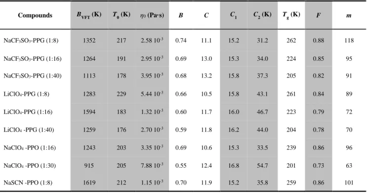
Table 1 Numerical values of the parameters in the VFT (BVFT, T0, η0), BSCNF (B, C) and WLF (C1, C2) equations for the polymeric systems.

Compounds B_VFT (K) T₀ (K) η⁰ (Pa·s) B C C₁ C₂ (K) T_g (K) F m

NaCF3SO3-PPG (1:8) 1352 217 2.58 10^-3 0.74 11.1 15.2 31.2 262 0.88 118 NaCF3SO3-PPG (1:16) 1264 191 2.95 10^-3 0.69 13.0 15.3 34.0 224 0.85 95 NaCF3SO3-PPG (1:40) 1113 178 3.95 10^-3 0.68 13.2 15.8 37.3 205 0.82 91 LiClO4-PPG (1:8) 1283 229 5.44 10^-3 0.66 10.5 15.8 43.1 261 0.84 89 LiClO4-PPG (1:16) 1594 183 1.32 10^-3 0.60 11.7 16.0 46.7 223 0.79 72 LiClO⁴ -PPG (1:40) 1259 176 2.70 10^-3 0.59 11.8 16.2 44.0 204 0.78 70 NaClO4 -PPO (1:16) 1243 203 3.35 10^-3 0.69 10.6 15.3 33.5 239 0.86 96 NaClO4 -PPO (1:30) 915 205 7.88 10^-3 0.55 12.4 16.8 54.7 201 0.73 63 NaSCN -PPO (1:8) 1619 212 1.15 10^-3 0.70 11.9 15.2 35.8 259 0.86 101

The numbers in the parenthesis in the compounds indicate the mole ratio. The experimental values of the glass transition temperature (Tg) [14-15] and the fragilities calculated from Eq. 3 (m) and 8 (F) are also given.

11 Figure Captions

Fig. 1 Examples of fitting of the experimental data with the a) BSCNF model, the VFT equation and the b) WLF equation.

Fig. 2 Relationship between the values of parameters B and C determined for different polymeric systems

.

Fig. 3 Relationship between the fragility index calculated from the BSCNF model, Eq. 3 and the value of the parameter C2 in the WLF equation.

Fig. 4 Relationship between the fragility index calculated from the BSCNF model, Eq. 3 and the fragility given by Eq. 8.

Fig. 5 Temperature dependence of viscosity for various compositions of polymeric ion conducting systems obtained from Eq. 1. Experimental values of different polymeric systems are shown by symbols. The behavior of SiO2 is also shown for comparison.

12

Fig. 1 (a)

13

Fig. 1 (b)

14

Fig. 2

15

Fig. 3

16

Fig. 4

17

Fig. 5