Eddy‑induced transport of the Kuroshio warm water around the Ryukyu Islands in the East China Sea
Author Yuki Kamidaira, Yusuke Uchiyama, Satoshi Mitarai
journal or
publication title
Continental Shelf Research
volume 143
page range 206‑218
year 2016‑07‑15
Publisher Elsevier
Rights (C) 2016 Elsevier Ltd.
Author's flag author
URL http://id.nii.ac.jp/1394/00000670/
doi: info:doi/10.1016/j.csr.2016.07.004
© 2017. This manuscript version is made available under the CC-BY-NC-ND 4.0 license http://creativecommons.org/licenses/by-nc-nd/4.0/
1 2
Eddy-induced transport of the Kuroshio warm water
3
around the Ryukyu Islands in the East China Sea
4 5 6 7
Yuki Kamidaira
1, Yusuke Uchiyama
2and Satoshi Mitarai
38 9 10
1. Corresponding author: Nuclear Science and Engineering Center, Japan Atomic 11
Energy Agency, Tokai, Ibaraki, Japan (email: [email protected]) 12
2. Department of Civil Engineering, Kobe University, Kobe, Hyogo, Japan (email:
13
3. Marine Biology Unit, Okinawa Institute of Science and Technology, Onna, 15
Okinawa, Japan (email: [email protected]) 16
17 18
Abstract
19
In this study, an oceanic downscaling model in a double-nested 20
configuration was used to investigate the role played by the Kuroshio warm current 21
in preserving and maintaining biological diversity in the coral coasts around the 22
Ryukyu Islands (Japan). A comparison of the modeled data demonstrated that the 23
innermost submesoscale eddy-resolving model successfully reproduced the 24
synoptic and mesoscale oceanic structures even without data assimilation. The 25
Kuroshio flows on the shelf break of the East China Sea approximately 150–200 km 26
from the islands; therefore, eddy-induced transient processes are essential to the 27
lateral transport of material within the strip between the Kuroshio and the islands.
28
The model indicated an evident predominance of submesoscale anticyclonic eddies 29
over cyclonic eddies near the surface of this strip. An energy conversion analysis 30
relevant to the eddy-generation mechanisms revealed that a combination of both 31
the shear instability due to the Kuroshio and the topography and baroclinic 32
instability around the Kuroshio front jointly provoke these near-surface 33
the shelf break. Both surface and subsurface eddies fit within the submesoscale, and 35
they are energized more as the grid resolution of the model is increased. An eddy 36
heat flux (EHF) analysis was performed with decomposition into the divergent 37
(dEHF) and rotational (rEHF) components. The rEHF vectors appeared along the 38
temperature variance contours by following the Kuroshio, whereas the dEHF 39
properly measured the transverse transport normal to the Kuroshio’s path. The 40
diagnostic EHF analysis demonstrated that an asymmetric dEHF occurs within the 41
surface mixed layer, which promotes eastward transport toward the islands.
42
Conversely, below the mixed layer, a negative dEHF tongue is formed that promotes 43
the subsurface westward warm water transport.
44 45
Key words: submesoscale eddy, Kuroshio, topography, East China Sea, ROMS 46
47
1. Introduction
48 49
Coral reefs are home to the most diverse range of marine life in the world. They 50
are of great importance to marine ecosystems, hosting favorable habitat to a wide 51
variety of flora and fauna. An estimated 25% of all marine life is supported by coral 52
reefs, even though they cover <0.1% of the world’s oceans and represent one of the 53
most fragile and endangered marine ecosystems in the world (e.g., Spalding et al., 54
2001). Coral reefs also represent a vital resource for humankind in terms of 55
tourism and fishing. Cesar et al. (2003) reported that coral reefs provide 56
approximately US$29.8 billion in net benefit streams per annum in goods and 57
services to world economies, including tourism (US$9.6 billion), fisheries (US$5.7 58
billion), and coastal protection (US$9.0 billion). Similarly, coral reefs have great 59
economic value in Japan, generating as much as US$1.6 billion per annum 60
domestically. In particular, the Ryukyu Islands, located in the subtropical region of 61
Japan that fringes the East China Sea (ECS; Fig. 1), have ecologically abundant coral 62
reefs situated at their northernmost end at the border between the Pacific and 63
Indian oceans. These corals lie within a region that supports the highest diversity of 64
indigenous species in the world.
65
Water temperature is widely known as a factor that has considerable effect on 66
coral growth. The ideal range of ambient temperature for reef corals is narrow;
67
most corals cannot survive in temperatures much below 16°C–18°C even for a few 68
weeks. High temperatures also have a serious effect on coral growth and can lead to 69
“coral bleaching,” a process that results in devastating mass mortality of the coral 70
during which they expel their symbiotic algae. Therefore, the habitat of coral is 71
generally restricted to a latitudinal band between 30°N and 30°S because 72
decreasing temperature follows increasing latitude.
73
The sea around the Ryukyu Islands in the ECS, located between 25°N and 30°N, 74
provides an environment for coral growth even though it lies at the northernmost 75
extreme of the habitable region. Major warm currents, such as the Kuroshio, allow 76
the development of reefs up to and beyond the ordinary habitable latitudinal limit.
77
These ocean currents play important roles in transporting coral larvae and warm 78
water to such areas, thus maintaining favorable environments for reef corals.
79
The Kuroshio, which is one of the world’s major western boundary currents of 80
the North Pacific subtropical gyre, enters the ECS from the east coast of Taiwan. It 81
turns northeastward and drifts along the continental shelf slope fringing the ECS 82
around the Ryukyu Islands (Qiu, 2001). The Kuroshio not only plays an essential 83
role in the meridional transport of large amounts of warm and salty tropical water 84
northward (e.g., Ichikawa and Beardsley, 1993; Ichikawa and Chaen , 2000;
85
Imawaki et al., 2001; Johns et al., 2001; Andres et al., 2008; Yang et al., 2011) but 86
also influences the regional climatic system of the ECS (e.g., Xu et al., 2011; Sasaki 87
et al., 2012). Temperature measurements recorded continuously by more than 100 88
thermometers in conjunction with satellite SST (sea surface temperature) 89
measurements have revealed that areas of high SST are formed off the middle of the 90
west coast of Okinawa Island because of the Kuroshio warm water (Nadaoka et al., 91
2001).
92
Several numerical studies have been undertaken to investigate the 93
physical processes and effects of the Kuroshio in the ECS. Guo et al. (2003) were 94
successfully demonstrated that the path and vertical structure of the Kuroshio in 95
the ECS are reproduced more realistically as the horizontal resolution of a model 96
increases on the basis of a triply nested ocean modeling using the Princeton Ocean 97
Model (Blumberg and Mellor, 1987). Based on a study using the Meteorological 98
Research Institute Community Ocean Model (Usui et al., 2006), Usui et al. (2008) 99
reported that frontal waves are generated as a result of the collisions between 100
anticyclonic mesoscale eddies with diameters at orders of 100 km. These eddies are 101
considered to have nontrivial influence on mass and heat transport between the 102
Kuroshio and the Ryukyu Islands. Their study suggested that eddy-induced lateral 103
Ryukyu Islands, because the main body of the Kuroshio is persistently located 105
approximately 150–200 km to the west of the islands, restricting its direct impact.
106
Recently, the effects of submesoscale eddies (at typical horizontal scales of 107
several to tens of km or less) on the mean oceanic structure, stratification, and 108
frontal processes have been studied actively to enhance our understanding of the 109
dynamic processes of the upper oceans (e.g., Boccaletti et al., 2007; Badin et al., 110
2011; Callies et al., 2015; Kunze et al., 2015). Capet et al. (2008) conducted a 111
high-resolution numerical experiment of the idealized California Current System 112
using the Regional Oceanic Modeling System (ROMS; Shchepetkin and McWilliams, 113
2005, 2008). They demonstrated that submesoscale eddies occur through 114
frontogenesis, which sharpens the surface density fronts, forming in the regions of 115
high strain on the flanks of mesoscale eddies, down to horizontal scales of a few 116
kilometers or less in association with strong vertical ageostrophic secondary 117
circulations in the surface boundary layer. A multiple nesting technique (e.g., 118
Marchesiello et al., 2003; Penven et al., 2006; Mason et al., 2010) has enabled 119
submesoscale eddy-resolving ocean modeling to investigate submesoscale stirring 120
and mixing in the upper oceans and associated material dispersal. For example, 121
Romero et al. (2013) conducted a Lagrangian particle tracking in the Santa Barbara 122
Channel, CA, USA, using quadruple-nested high-resolution ROMS modeling with a 123
75-m horizontal grid size. Uchiyama et al. (2014) performed a Eulerian passive 124
tracer tracking for sewage outfalls in the Santa Monica and San Pedro bays in the 125
Southern California Bight using a similar quadruple-nested downscaling ocean 126
modeling. Both studies exhibited anisotropic along- and cross-shelf dispersal of 127
material concentrations and particles on the continental shelves and nearshore 128
areas, markedly dominated by submesoscale-eddy mixing. In addition to those 129
studies focusing on the eastern boundary currents, several other studies have 130
investigated the western boundary currents, such as the Kuroshio and its 131
extension region off Japan (e.g., Sasaki et al., 2014) and the Gulf Stream off the U.S.
132
east coast (e.g., Gula et al., 2014). However, the influence of submesoscale eddies on 133
upper-ocean dynamics and the resultant dispersal and transport of materials, 134
including the Kuroshio-derived warm water, nutrients, and coral larvae, has not yet 135
been investigated adequately around the Ryukyu Islands in the ECS.
136
Another important aspect of the Ryukyu Islands is their upheaved shallow 137
topography on the relatively deep Ryukyu Trough, which is situated on the eastern 138
side of the ECS continental shelf break where the Kuroshio persistently flows 139
northeastward. The islands obstruct the westward-propagating mesoscale eddies 140
that detach from the Kuroshio recirculation (Nakamura et al., 2009). Therefore, this 141
obstruction may result in the emergence of unique turbulence such as island wakes 142
and associated eddy shedding, as has been investigated in the Southern California 143
Bight (e.g., Dong and McWilliams, 2007). These geographical configurations are 144
presumed to set preferable conditions for the development of submesoscale-eddy 145
mixing through baroclinic and barotropic instability due to the Kuroshio fronts and 146
topographic shear within the study area.
147
In the present study, a submesoscale-eddy-resolving numerical 148
experiment was conducted for the area around the Ryukyu Islands. The study was 149
based on a double-nested ocean downscaling configuration using the ROMS, 150
embedded in the assimilative Japan Coastal Ocean Predictability Experiments 151
(JCOPE2) oceanic reanalysis (Miyazawa et al., 2009) with atmospheric forcing from 152
the assimilative GPV-GSM (e.g., Roads, 2004) and MSM (e.g., Isoguchi et al., 2010) 153
reanalysis products. The innermost ROMS model domain (the principal focus of this 154
analysis) had 1-km horizontal grid spacing, which was suitably fine for full 155
representation of submesoscale activities (Capet et al., 2008). Particular attention 156
was given to the model’s reproducibility, statistical description of intrinsic 157
submesoscale eddies, possible mechanisms for eddy inducement, and influence of 158
the eddies on the lateral mixing that promotes transport of the Kuroshio water 159
toward the islands. The remainder of this paper is organized as follows. A 160
description of the modeling framework used for the hindcast experiment for the 161
years 2010–2013 is given in Sec. 2. Section 3 illustrates an extensive comparison 162
between the model results and field observation and satellite altimetry data in order 163
to validate the model’s capability of reproducing the Kuroshio and 3-D oceanic 164
structure. Section 4 considers the impact of downscaling, which is followed by 165
analyses of both the energy conversion and instability relevant to eddy kinetic 166
energy in Sec. 5 and of the heat flux in Sec. 6. Conclusions are given in Sec. 7 167
168
2. Model configuration
169 170
Figure 1 shows the numerical domains of the oceanic downscaling model 171
in a double-nested configuration embedded in the JCOPE2 (Miyazawa et al., 2009) 172
domain. The JCOPE2 is a numerical reanalysis product for the northwestern Pacific 173
floats using 3D-VAR. The JCOPE2 product is provided as daily averaged sea surface 175
height (SSH), temperature, salinity, and meridional and zonal horizontal current 176
velocities. We relied on a one-way offline nesting approach (Mason et al., 2010) to 177
reduce the horizontal grid size from approximately 10 (JCOPE2) to 3 km 178
(ROMS-L1), and ultimately, down to 1 km (ROMS-L2). The parent ROMS domain 179
(ROMS-L1) had a horizontal size of 2304 × 2304 km with uniformly square 3-km 180
grid spacing and vertically stretched 32 -layers, designed to encompass a wide 181
area to consider all possible impacts of the Kuroshio flowing in from the Taiwan 182
Strait and the Luzon Strait. The climatological monthly freshwater discharge of the 183
Yangtze River into the ECS, which is reported to range approximately between 184
838-907 km3/yr (e.g., Dai et al., 2009), was taken into account. The innermost 185
ROMS-L2 domain was 832 × 608 km with 1-km horizontal resolution and 32 186
vertical -layers, which covered the entire chain of the Ryukyu Islands, from the 187
Amami Islands of Kagoshima Prefecture in the north to the Yaeyama Islands of 188
Okinawa Prefecture in the south. Table 1 lists the numerical configuration of the 189
ROMS models.
190
The outermost boundary and initial conditions of ROMS-L1 were obtained 191
from the spatiotemporally interpolated fields of the daily averaged JCOPE2 data. The 192
model topography was obtained from the SRTM 30 Plus product (SRTM: Shuttle 193
Radar Topography Mission; Rodriguez et al., 2005; Becker et al., 2009), which 194
covers the global ocean at 30 geographic arc seconds, or roughly 1 km. We utilized 195
the QuikSCAT-ECMWF blended wind (e.g., Bentamy et al., 2006) for 2005–2007 and 196
the JMA GPV-GSM product (JMA: Japan Meteorological Agency, GPV-GSM: grid point 197
value of the Global Spectral Model) with horizontal resolution of 0.2° × 0.25° for 198
2008–2013 for surface momentum forcing, depending on the availability of these 199
data sets. Surface heat, freshwater and radiation fluxes were taken from the COADS 200
(Comprehensive Ocean–Atmosphere Data Set; Woodruff et al., 1987) monthly 201
climatology. The 20-day averaged JCOPE2 data were applied to the SST and sea 202
surface salinity (SSS) restoration with a time scale of 90 days to correct long-term 203
biases caused by the imposed climatological surface fluxes. The monthly 204
climatology of the major river discharges in Dai et al. (2009) was applied for the 205
Yangtze River. A four-dimensional TS nudging (a.k.a. robust diagnostic; e.g., 206
Marchesiello et al., 2003) with a weak nudging time scale of 1/20 per day was 207
applied to the 10-day averaged JCOPE2 temperature and salinity fields for 208
consistency of the Kuroshio path reproduced by the ROMS-L1 with that of JCOPE2.
209
The L1 model was used for more than eight years from January 1, 2005 until 210
September 14, 2013, UTC.
211
The innermost L2 model was initialized and forced along the boundary 212
perimeters by the spatiotemporally interpolated daily averaged L1 output. The 213
hourly output of the JMA GPV-MSM (Mesoscale Model) reanalysis, which 214
encompasses the entire L2 domain with horizontal resolution of 0.05° × 0.0625°, 215
was used for the L2 model instead of the GPV-GSM. Similar to the L1 model, SST and 216
SSS restoration for surface flux correction was included. The other numerical 217
conditions were the same as for the L1 model. Hence, the L2 model was run freely 218
without any assimilation such as the TS nudging that could interfere with the 219
spontaneous development and decay of intrinsic eddies. We note that the present 220
model does not include tidal forcing since it is considered to have minor effects on 221
mean and eddy field in such an open ocean configuration. For instance, Romero et al.
222
(2013) pointed out that dispersal and mixing in Santa Barbara Channel, CA, USA, 223
are dominated much prominently by submesoscale stirring, not by tides. The L2 224
model computational period was approximately 33 months, from December 27, 225
2010 to September 14, 2013, UTC. The statistical analyses conducted in the present 226
study exploit the model results for the same period between March 27, 2011 and 227
September 14, 2013, unless otherwise noted.
228 229
3. Model Validation
230 231
In this section, we compare the model results with satellite, in situ 232
observations, and the assimilative JCOPE2 reanalysis. Figure 2 shows the time 233
series of the volume-averaged surface kinetic energy (KE) for the three model 234
results (i.e., JCOPE2, ROMS-L1, and ROMS-L2). The volume average is taken over the 235
entire ROMS-L2 domain from the surface to a depth of 400 m, encompassing the 236
region in which the Kuroshio main body is most influential. The temporal variations 237
of the upper-ocean KE in the three models are similar. Given the fact that JCOPE2 is 238
assimilated with multiple satellite altimetry data, SST, ARGO, and in situ mooring 239
data, the two ROMS models provide realistic estimates of the near-surface eddy 240
activities. The ROMS-L2 generally yields slightly larger KE than the other cases 241
because it is a submesoscale eddy-resolving model that results in more energetic KE, 242
while retaining adequate seasonal variability. This result is achieved if the L1 model 243
dissipate KE appropriately for realistic replication of the Kuroshio’s behavior.
245
Otherwise, the KE in the L1 model increases significantly with unrealistically large 246
meandering of the Kuroshio path (not shown). Conversely, the L2 model with the 247
assimilated L1 boundary forcing behaves favorably, as shown in Fig. 2, without any 248
controls such as TS nudging.
249
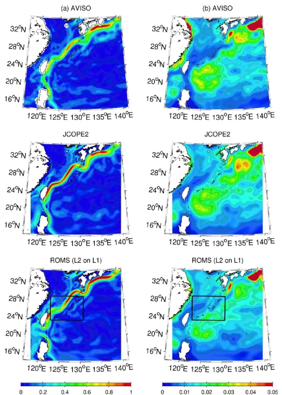
Extensive model-data comparisons are performed using satellite altimetry 250
data and JMA observations to demonstrate the reproducibility of the double-nested 251
ROMS model. For validating the mean structure and temporal variance of the surface 252
currents, including the Kuroshio, we exploited the gridded composite of multiple 253
satellite altimetry data provided by AVISO (e.g., Traon et al., 1998). The delayed-time 254
AVISO-SSH data set is available daily with horizontal spacing of 1/4°. The magnitude 255
of the time-averaged geostrophic current velocity, estimated from the AVISO-SSH, 256
exhibits comparable magnitude with the corresponding patterns of the JCOPE2 and 257
ROMS-L2 on the L1 (Fig. 3). However, the Kuroshio intrusion into the South China 258
Sea from Luzon Strait in the ROMS-L1 model occurs more apparently than that in 259
AVISO and JCOPE2 where the westward meander is weakened with generating a 260
leaped eddy or a ring. The looping in the Luzon Strait could be realistic since it has 261
been reported both observationally and computationally (e.g., Centurioni et al., 262
2004 and Miyazawa et al., 2004). Nevertheless, Luzon Strait is located sufficiently 263
far from the study area, and thus we conclude the plots of the ROMS velocity 264
magnitude also show reasonable agreement with the Kuroshio path of the other two 265
data sets. The SSH variance is viewed as a proxy that measures the intensity of the 266
temporal variability in synoptic and mesoscale signals mostly due to eddies and the 267
Kuroshio meanders. The ROMS-derived SSH variance reproduces several important 268
features with equivalent magnitudes to the AVISO data. For instance, the variance is 269
smaller on the persistent Kuroshio path on the western side of the Ryukyu Islands, 270
compared with the other side, where the westward-traveling Rossby waves and 271
mesoscale eddies collide with the topographic ridge around the islands. Another 272
energetic area commonly arises north of 29°N, off the southwest coast of Kyushu 273
Island.
274
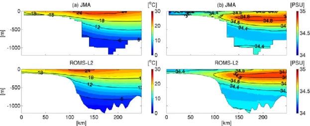
The modeled stratification is subsequently compared with in situ 275
observations from the vertical section along the PN Line transect (e.g., Miyazawa et 276
al., 2009), indicated by the thick black lines in Fig. 1. The PN Line measurements 277
comprise 16 CTD (conductivity, temperature and depth) casts that have been 278
obtained seasonally since 1972 by JMA research vessels. As this transect favorably 279
transverses the Kuroshio path in the ECS, we can estimate the volume transport 280
across the PN Line. Comparisons of the seasonally averaged temperature and 281
salinity clearly illustrate that the present model is capable of reproducing the 282
observed stratification, not just in spring (Fig. 4) but in all seasons (not shown). A 283
tilted thermocline and halocline are formed toward the ECS shelf region with 284
subsurface salinity maxima in the trough region. Table 2 summarizes the modeled 285
and observed volume flux (transport) in Sverdrup along the PN Line. The observed 286
volume fluxes are estimated geostrophically from the slope of the isobaric surface, 287
based on the seasonal climatology of the temperature and salinity (Fig. 4) by 288
assuming the transport vanishes at 1000 m depth. The volume fluxes obtained by 289
the models principally contain the ageostrophic component, which results in slightly 290
larger transport than those observed. However, the modeled volume fluxes 291
adequately capture the observed seasonal variability, such as the increase in 292
summer and the decrease in fall. Interestingly, the ROMS-L2, with the finest grid 293
resolution without TS nudging, provides a better estimate of the transport 294
(compared with the observations) than that evaluated using the coarser-resolution 295
models (viz., ROMS-L1 and JCOPE2), both of which employ data assimilation to some 296
extent. This is likely attributable to the occurrence of an appropriate spontaneous 297
flux adjustment in the ROMS-L2 through submesoscale lateral mixing and 298
associated dissipation at the resolved scales of the mean KE around the Kuroshio 299
path. In summary, the presented double-nested ROMS model is shown satisfactorily 300
capable of reproducing the mesoscale behavior of the Kuroshio and the mean 3-D 301
oceanic structure.
302
4. Downscaling effects
303 304
The unassimilated L2 model is capable of fully resolving submesoscale 305
eddies, whereas the L1 and JCOPE2 are submesoscale-permitting (Capet et al., 306
2008). Therefore, eddy activity should be enhanced by the grid refinement of the 307
downscaling via the increase and strengthening of the resolved eddies. To examine 308
the downscaling effects, surface eddy kinetic energy (EKE), Ke, can be estimated as 309
follows:
310
, (1) 311
where (u, v) is the horizontal velocity and the overbar represents an 312
ensemble-averaging operator. The variables assigned with the prime are the 313
fluctuating eddy components obtained by removing the seasonal variations with a 314
low-pass Butterworth filter in the frequency domain (the first and last 10% of the 315
analysis period cannot be used because of the Butterworth filter’s properties).
316
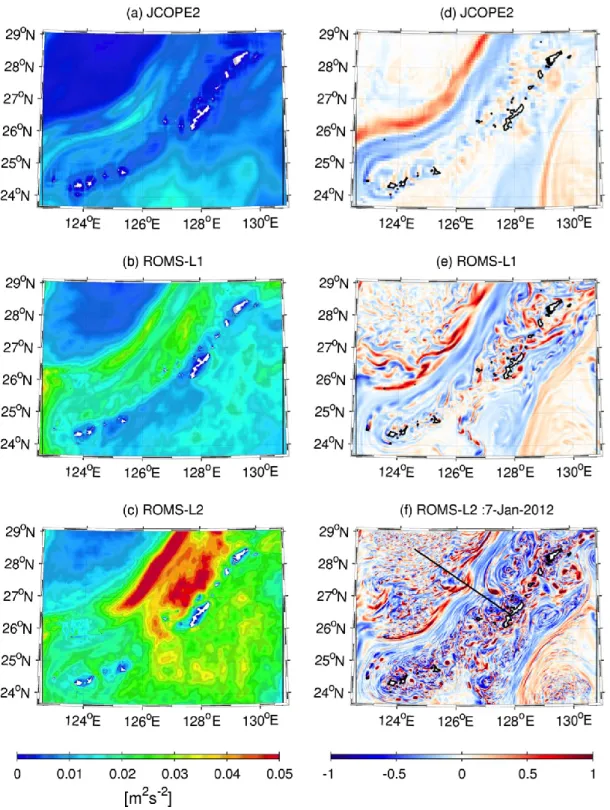
Figure 5a–c demonstrates that the surface EKE increases markedly as the model 317
grid spacing decreases from 10 to 3 and to 1 km. The higher EKE mostly emerges in 318
two distinct regions: one is on the Kuroshio axis and the other is on its eastern side, 319
close to Okinawa (Main) Island.
320
Figure 5d–f illustrates the daily averaged, surface relative vorticity 321
normalized by the background rotation f (the Coriolis parameter), viz., representing 322
the emergence of mesoscale and submesoscale eddies in each model. The variable 323
ζ/f is also known as the vortical Rossby number, the absolute value of which is 324
greater than unity when ageostrophy is more evident. Vorticity is generally 325
distributed as streaks and filaments around the Kuroshio axis where the change of 326
sign occurs. However, enclosed circular eddies are dominant away from the axis, in 327
particular, in the two ROMS model results. The two distinctive high EKE (Ke) regions 328
in Fig. 5a–c are consistent with these vorticity distributions. As the resolution 329
becomes finer, the extent and magnitudes of the resolved vortices become 330
prominently diversified and enhanced, coinciding with the high EKE region on the 331
eastern side of the Kuroshio (Fig. 5a–c). The higher-resolution model renders 332
smaller submesoscale eddies that typically have diameters of several kilometers.
333
We notice that negative vorticity, viz., counter-clockwise-rotating cyclonic 334
eddies, develops more vigorously and widely on the east side of the Kuroshio than 335
on the other side, where positive vorticity dominates. The innermost model with the 336
highest resolution (ROMS-L2) captures the negative vorticity that is retained 337
significantly on the eastern side of the Kuroshio, while the centrifugally stable 338
positive vorticity is attenuated rather quickly there. The ROMS-L2 model has the 339
smallest eddies and the largest negative vorticity near the islands. This negative bias 340
near the islands, in the direction transverse to the Kuroshio path, is presumably 341
caused by the increase of the resolved eddies with the increased model resolution.
342
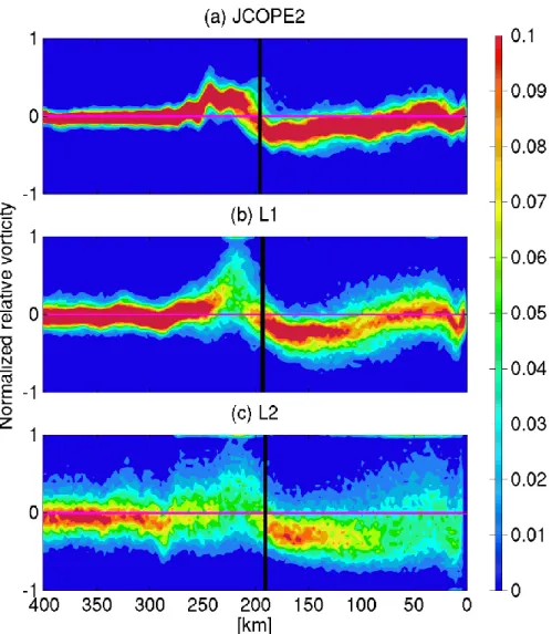
To confirm this negative bias quantitatively, the probability density function (PDF) 343
of the normalized relative vorticity (ζ/f) at the surface was determined as a function 344
of the westward transverse distance from Okinawa Island along transect AA’, as 345
shown in Fig. 5f. This transect is defined normal to the mean Kuroshio axis, 346
averaged over the computational period, which is inclined at 35° relative to the 347
geographical coordinate. Figure 6 indicates that the finer-resolution models yield 348
stronger vortices with gentler PDF slopes along the ordinates. Although the PDFs 349
are distributed nearly symmetrically with respect to the Kuroshio axis, they peak at 350
ζ/f < 0 on the eastern side of the Kuroshio axis, even adjacent to Okinawa Island.
351
This negative bias on the east is most evident at the highest resolution. On the west 352
of the Kuroshio, large positive vorticity appears immediately next to the Kuroshio, 353
while the PDF peaks converge to zero away from the axis to the west. In summary, 354
the Ryukyu Islands are considered to enhance both intensity and fluctuations of the 355
anticyclonic negative vorticity on the eastern side of the Kuroshio axis. However, on 356
the other side, anticyclones and cyclones compete with the activated positive 357
vorticity near the Kuroshio axis. This transverse asymmetry is a unique structure 358
that characterizes the eddy field of the study area, which is perhaps related to both 359
the topographic ridge near the island chain and the continental shelf break along 360
which the Kuroshio persistently drifts (Fig. 1), as well as frontal processes 361
associated with the Kuroshio warm water.
362 363
5. Energy conversion analysis
364 365
Energy conversion rates in the eddy kinetic energy (Ke) conservation 366
equation are often used to quantify the relative importance of instability and 367
eddy-mean interaction mechanisms (e.g., Marchesiello et al., 2003; Dong et al., 368
2006; Klein et al., 2008). If the conversion of mean kinetic energy to eddy kinetic 369
energy KmKe (viz., barotropic conversion rate) is positive, it implicates the 370
occurrence of shear instability in the extraction of Ke to energize eddies. If the 371
conversion of eddy potential energy to eddy kinetic energy PeKe (viz., baroclinic 372
conversion rate) is positive, baroclinic instability is expected. We focus on these two 373
primary quantities, as expressed in the following equations, in the investigation of 374
the stimulation mechanisms of Ke: 375
, (2) 376
, (3) 377
where (x, y, z) are the horizontal and vertical coordinates, w is the vertical velocity, ρ 378
is the density of sea water, ρ0 = 1027.5 kgm−3 is the Boussinesq reference density, 379
and g is gravitational acceleration. The vertically integrated KmKe, PeKe, and Ke (EKE) 380
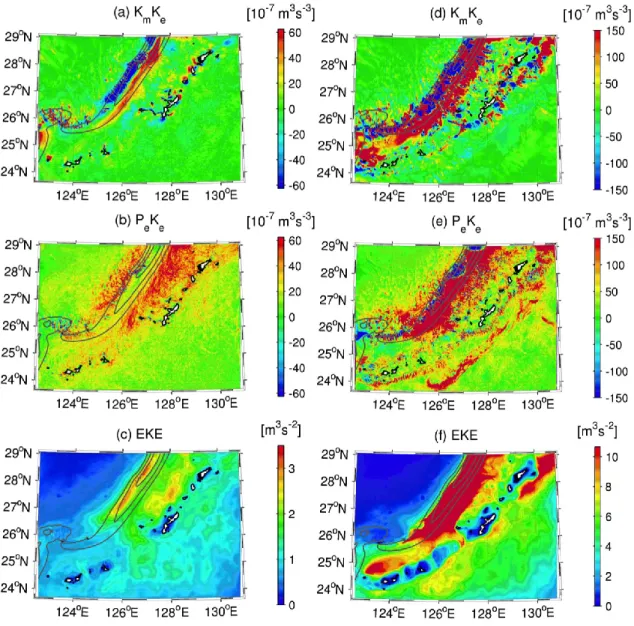
over the mixed layer from the ROMS-L2 model are plotted in Fig. 7a–c. The 381
averaged mixed-layer depth estimated by the KPP model (Large et al., 1994) used in 382
the ROMS is approximately 50 m in the L2 domain. The mixed-layer integrated PeKe
383
is positive almost everywhere with two distinctly high regions around the Kuroshio 384
axis and the neighboring flank on the eastern side to the islands (Fig. 7b). This PeKe
385
distribution illustrates the importance of baroclinic instability in the vorticity 386
generation within these two regions. In contrast, an axisymmetric pair of large 387
positive and negative areas of KmKe can be observed in the narrow strips on both 388
sides of the Kuroshio, representing the lateral shear instability induced by the 389
Kuroshio (Fig. 7a). In general, the regions with positive PeKe and positive KmKe
390
coincide with the areas of high Ke (Fig. 7c).
391
The area of highly positive PeKe is distributed widely between the 392
Kuroshio path and the Ryukyu Islands, whereas the highly positive KmKe appears 393
mostly near the Kuroshio and on the western side of the islands near the 394
topography. The vertically integrations of KmKe, PeKe, and Ke over the mixed layer 395
along the transect are plotted in Fig. 8. Consistent with Fig. 7a–c, PeKe is positive 396
and larger than KmKe almost everywhere along the transect, indicating that 397
baroclinic instability is the dominant mechanism for eddy generation near the 398
surface, especially, on the eastern side of the Kuroshio path where high values of Ke
399
appear. Therefore, it is manifest that the negative vorticity on the eastern side of the 400
Kuroshio (Fig. 5f) is provoked by a combination of the lateral shear affected by the 401
Kuroshio, topographic eddy shedding near the islands, and baroclinic instability due 402
to the Kuroshio front. The negative KmKe on the western side of the Kuroshio 403
suggests that positive vorticity is suppressed by the lateral shear through an inverse 404
energy cascade while baroclinically destabilized by the competing positive PeKe. 405
The EKE (Ke) budget is examined further for the subsurface water, where 406
the Kuroshio is influential, by vertical integration of KmKe, PeKe, and Ke from the 407
surface down to a depth of 1200 m with the L2 result (Fig. 7d–f). The L2 model 408
detects large positive barotropic and baroclinic conversion rates near the Kuroshio 409
that coincide with the region of high Ke . In addition, an increase of the subsurface 410
PeKe and resultant intensification of Ke are evident on the eastern side of the islands, 411
due to a branch of the Kuroshio known as the Ryukyu (Under) Current (e.g., Kawabe, 412
2001; Andres et al., 2008). This large PeKe could induce further subsurface 413
westward lateral mixing and intrusion of the Ryukyu Current. However, this is 414
beyond the scope of the present study and it will be examined elsewhere. The 415
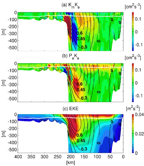
subsurface structure on the western side of the islands is illustrated in Fig. 9 with 416
respect to the vertical cross-section along transect AA’ (see Fig. 5f). The Kuroshio 417
main body is inclined on the shelf slope with a mean streamwise velocity of >0.2 418
m/s, even at 600 m depth. High Ke is distributed widely near the surface to the east, 419
coinciding with the positive KmKe near the Kuroshio and positive PeKe extending 420
between the Kuroshio and Okinawa Island. Conversely, high Ke is mostly confined 421
along the shelf break from the surface to 400 m depth to the west, where both KmKe
422
and PeKe increase in magnitude with the sign change.
423
Below the mixed layer, the Kuroshio is squeezed strongly against the shelf 424
slope on the eastern side, which provokes large velocity shear and thus large 425
positive KmKe, which is associated with the shear instability due to topographic eddy 426
shedding. Around the inclined Kuroshio core, competing large positive PeKe and 427
large negative KmKe are formed simultaneously below the mixed layer down to a 428
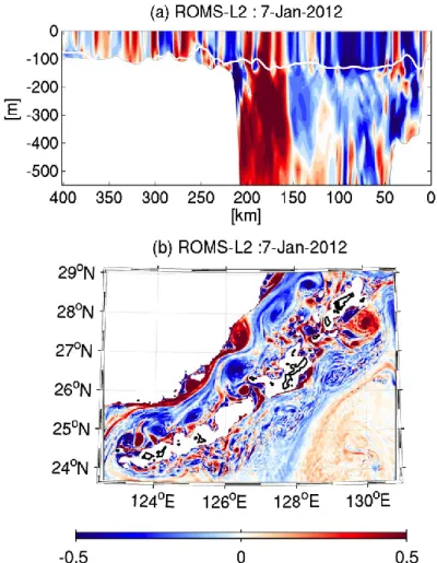
depth of 600 m. Figure 10 shows a snapshot of the daily averaged, normalized 429
relative vorticity (ζ/f) field in the vertical section along the transect and in the 430
horizontal section at z = −400 m from the L2 model. In Fig. 10a, negative vorticity 431
(anticyclonic submesoscale eddies) appears dominantly near the surface on the 432
eastern side of the Kuroshio toward Okinawa Island, while positive cyclonic vorticity 433
appears around the Kuroshio core from the surface down to depths beyond 500 m 434
along the shelf slope. The diameter of this cyclone is approximately 50 km, which 435
still fits within a typical submesoscale range. In Fig. 10b, cyclonic eddy shedding 436
occurs quasi-periodically from the shelf slope topography. Therefore, a combination 437
of topographic shear and baroclinic instability promotes the near-surface 438
anticyclonic eddies and subsurface cyclonic eddies, both of which are submesoscale.
439
440
6. Heat flux analysis
441 442
The submesoscale anticyclonic eddies induced by the Kuroshio are 443
anticipated to promote eastward material transport to the west coast of Okinawa 444
Island through lateral eddy mixing. To quantify this effect, we assessed the lateral 445
turbulent mixing of a tracer (i.e., heat) in the upper ocean. The time-averaged, 446
vertically integrated heat (potential temperature) transport equation is 447
represented as (e.g., Marchesiello et al., 2003):
448
, (4) 449
where T is potential temperature, Q is the sea surface heat flux, D is the 450
parameterized vertical and horizontal subgrid-scale mixing of heat, h is depth, and 451
is surface elevation. We focus on the advective transport by eddying flow, which is a 452
divergence of lateral eddy heat fluxes (EHFs) F:
453
F = (Fx, Fy)=( , ), (5) 454
where Cp = 4000 Jkg−1°C−1, which is the heat capacity of seawater at a constant 455
pressure. To quantify the eddy heat transport to the islands, a divergent component 456
of the EHF is evaluated. The EHF can be decomposed into divergent and rotational 457
components using Helmholtz’s theorem (e.g., Aoki et al., 2013) such that 458
F = k ×∇ψ +∇φ rEHF + dEHF, (6) 459
where k is a vertical unit vector, and ψ and φ are scalar quantities similar to a 460
streamfunction and a velocity potential, respectively. We introduce the notation 461
where rEHF and dEHF are the rotational and divergent components of the EHF. This 462
decomposition is conducted by numerically solving the Poisson equation (6) with 463
Neumann boundary conditions.
464
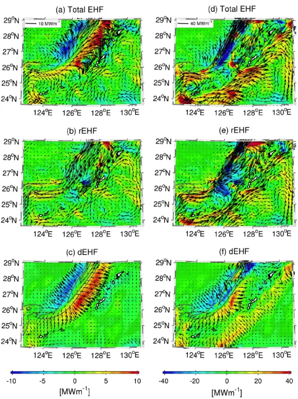
The mixed-layer integrated EHF, rEHF, and dEHF vectors, superimposed 465
on their transverse component relative to the mean Kuroshio path from the L2 466
result, are plotted in Fig. 11a–c. The total EHF (Fig. 11a) is properly decomposed 467
into the rEHF (Fig. 11b) and dEHF (Fig. 11c). The rEHF vectors mainly follow the 468
prevailing direction of the northeastward-drifting Kuroshio path with recurring 469
southwestward eddy heat transport near the islands. The eddy heat transport in the 470
opposite direction to the Kuroshio near the islands is obviously due to a mesoscale 471
secondary circulation often known as the Kuroshio Counter Current, as reported in 472
previous studies (e.g., Qiu and Imasato, 1990). However, the mixed-layer integrated 473
dEHF properly measures the contribution normal to the Kuroshio axis, which 474
manifests the lateral eddy heat transport toward the islands. Figure 11c also 475
demonstrates that the near-surface heat transport to the islands occurs more 476
strongly on the eastern side of the Kuroshio, although a weaker northwestward heat 477
transport occurs on the other side. This near-surface heat transport toward the 478
islands is obviously induced by anticyclonic submesoscale eddies developed around 479
the Ryukyu Islands (Sec. 4).
480
Figure 11d–f shows the vertically integrated EHF vectors from the 481
surface to 1200 m depth. In general, the vectors are similar to those integrated over 482
the mixed layer, although several substantial differences can be observed. The total 483
EHF and rEHF occurs mainly in the direction of the Kuroshio path, whereas the 484
major transport bifurcates around Ishigaki Island, which is located near the 485
lower-left corner of the domain, forming the Ryukyu Current EHF branch that 486
passes on the eastern side of Okinawa Island. As this subsurface branch drifts close 487
to several islands, including Okinawa Island, the influence of the Kuroshio on the 488
Ryukyu Islands is partially brought by this under current. Other differences include 489
the attenuated positive across-Kuroshio transport (dEHF) between the Kuroshio 490
and Okinawa Island and the southeastward subsurface dEHF on the eastern side of 491
the islands due to the Ryukyu Current. These findings illustrate that the 492
near-surface dEHF brings the Kuroshio warm water to the islands, whereas the 493
subsurface dEHF affects them in a different way.
494
Figure 12 shows cross-sectional plots of mean temperature, temperature 495
variance, and dEHF (eastward positive to Okinawa Island) along the transect. The 496
mean thermocline and mixed-layer depths become shallower toward the ECS shelf 497
from Okinawa Island. However, the Kuroshio induces additional effects such that the 498
mean thermocline is inclined to shallow both toward the ECS shelf and toward 499
Okinawa Island, with a near-surface bulge of warm water around the Kuroshio axis.
500
The maximum lateral temperature gradient is formed adjacent to the Kuroshio core 501
that is inclined on the shelf slope. The overall stratification is increased by this 502
inclined thermocline, established from the thermal wind relation with the 503
cross-sectional velocity structure due to the Kuroshio. Although the across-Kuroshio 504
negative dEHF is formed in the west, which penetrates to a depth of 400 m along 506
the slope (Fig. 12c). The temperature variance (Fig. 12b) is large where the dEHF 507
and Ke (see Fig. 8c) are consistently large. Interestingly, the temperature variance is 508
increased around the mean mixed-layer depth on the ECS shelf, perhaps provoked 509
by temporal fluctuations of the thermocline.
510
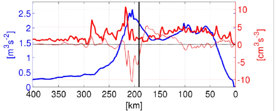
The mixed-layer integrated dEHF along the transect (Fig. 13) indicates 511
that energetic lateral eddy heat transport is induced within and around the surface 512
mixed layer, leading to the zonal transport of the Kuroshio warm water. The positive 513
eddy flux develops more strongly on the eastern side of Kuroshio than does the 514
negative flux on the other side in the mixed layer. Nevertheless, the largest 515
temperature variance emerges between the Kuroshio and the slope where the 516
tongue of negative dEHF exists. The subsurface topographic eddy shedding on the 517
slope (Fig. 10) promotes this tongue of negative dEHF, which results in subsurface 518
westward heat transport via the warm water brought up from the bottom of the 519
Kuroshio to the ECS shelf. As a consequence of all these processes, lateral eddy heat 520
transport occurs asymmetrically relative to the Kuroshio path.
521 522 523
7. Conclusions
524 525
Eddy-induced lateral mixing due to the Kuroshio around the Ryukyu 526
Islands in the ECS was investigated using a double-nested ROMS model that 527
downscales the assimilative JCOPE2 oceanic reanalysis to the innermost 528
submesoscale eddy-resolving model with 1-km grid spacing. An extensive 529
model-data comparison was performed against field observations and satellite 530
altimetry data to demonstrate the model’s capability of reproducing the Kuroshio 531
and 3-D oceanic structure. The model-data comparison demonstrated that the 532
elaborated innermost high-resolution ROMS-L2 model successfully reproduced 533
mesoscale structures spontaneously without any data assimilation.
534
The L2 models simulated significant negative vorticity bias, comprising 535
anticyclonic mesoscale and submesoscale eddies, on the western side of the islands.
536
The PDF of the normalized relative vorticity along the transect normal to the mean 537
Kuroshio path supported this asymmetric appearance of negative vorticity. Positive 538
vorticity was confined mostly to the vicinity of the Kuroshio, while the peak vorticity 539
PDF converged to zero (viz., almost no positive and negative bias) toward the ECS 540
shelf. These results reinforce the speculation that eddies are generated because of 541
interactions between the Kuroshio warm water and the unique local topography, 542
including the ridge of the islands to the east and the ECS continental shelf break to 543
the west, along which the Kuroshio persistently flows.
544
The energy conversion analysis focusing on the barotropic and baroclinic 545
conversion rates suggested that the near-surface anticyclonic negative vorticity on 546
the eastern side of the Kuroshio and the subsurface cyclonic positive vorticity on the 547
western side are generated via the combination of shear instability and baroclinic 548
instability, both of which are evidently influenced by the Kuroshio. Conversely, the 549
negative barotropic conversion rate, which appeared near the Kuroshio axis, 550
suggested that cyclonic positive vorticity is suppressed by the Kuroshio’s lateral 551
shear near the surface. The resultant surface EKE is thus also asymmetric with 552
respect to the Kuroshio, with greater EKE distributed widely on the eastern side of 553
the path. However, the subsurface water below the mixed layer reflected a 554
pronouncedly different energy balance. The magnitude of the subsurface barotropic 555
conversion rate is large on the shelf break, where a positive conversion rate 556
appears near the slope, whereas a negative rate appears to the east, where it 557
competes with a large positive baroclinic conversion rate.
558
The heat flux analysis solidly explained that these eddies promote lateral 559
material transport from the Kuroshio. Helmholtz decomposition was introduced to 560
the EHFs to evaluate the rotational and divergent components of the EHF, rEHF, and 561
dEHF. The decomposed rEHF detected the contribution from the EHFs that mainly 562
follow the Kuroshio and the anticyclonic recurring secondary circulation referred to 563
as the Kuroshio Counter Current. Conversely, the dEHF measured the contribution 564
normal to the Kuroshio axis, which represents the transverse eddy-induced 565
transport to the islands. The surface lateral eddy heat transport occurs 566
asymmetrically relative to the Kuroshio axis, with greater transverse eastward 567
transport than toward the ECS shelf. This occurs because of the more energetic 568
anticyclonic submesoscale eddies on the eastern side of the Kuroshio. Consistent 569
with the subsurface energy conversion rates, the depth-integrated EHFs were 570
visibly different from those near the surface. Although the depth-integrated EHF 571
and rEHF occur mainly in the direction of the Kuroshio path, the across-Kuroshio 572
transport (viz., dEHF) showed that they can be enhanced significantly near the 573
surface, which promotes warm water transport in both transverse directions 574
uniquely on the shelf slope and thus the subsurface warm water is brought upward 576
along the slope toward the ECS shelf. This negative dEHF tongue was attributed to 577
subsurface eddies generated by a combination of the baroclinic and shear instability, 578
according to the energy conversion analysis. These subsurface eddies are evidently 579
shed on the ECS shelf slope down to a depth of 600 m as energetic cyclonic 580
submesoscale eddies.
581
The present study clarified that the Kuroshio warm water undoubtedly 582
influences the biologically diverse ecosystems with abundant corals that have 583
formed around the Ryukyu Islands through mechanical intrusion. Based on the 584
modeling results, it was established that the Kuroshio-derived waters approach the 585
islands in at least three ways: 1) by transverse eddy-induced lateral mixing near the 586
surface, 2) via a clockwise recurring flow known as the Kuroshio Counter Current, 587
and 3) via a subsurface pathway associated with the Ryukyu Current. This study 588
focused primarily on the first mechanism that is accompanied by subsurface 589
submesoscale eddy transport toward the ECS shelf, induced by topographic eddy 590
shedding on the slope. Further analysis will be required to elucidate the detailed 591
mechanisms leading to the other two processes.
592 593
Acknowledgements
594
We are grateful to James C. McWilliams, Alexander F. Shchepetkin, and M.
595
Jeroen Molemaker of UCLA and Mayumasa Miyazawa of JAMSTEC for their help and 596
comments on the numerical modeling. We are also grateful to Shohei Nakada of 597
OIST for his help on the organizing JMA’s research vessels data. This study was 598
supported by JSPS Grant-in-Aid for Scientific Research C and B (KAKENHI grant 599
numbers: 24560622 and 15H04049).
600 601
References
602 603
1) Andres, M., Park, J., Wimbush, M., Zhu, X., Chang, K. and Ichikawa, H. 2008. Study 604
of the Kuroshio/Ryukyu Current System Based on Satellite-Altimeter and in situ 605
Measurements. J. Oceanogr., 64, 937-950.
606
2) Aoki, K., Minobe. S., Tanimoto, Y. and Sasai, Y. 2013. Southward Eddy Heat 607
Transport Occurring along Southern Flanks of the Kuroshio Extension and the 608
Gulf Stream in a 1/108 Global Ocean General Circulation Model. J. Phys. Oceanogr., 609
43, 1899-1910.
610
3) Badin, G., Tandon, A. and Mahadevan, A. 2011. Lateral Mixing in the Pycnocline 611
by Baroclinic Mixed Layer Eddies. J. Phys. Oceanogr., 41, 2080-2101.
612
4) Becker, J. J., Sandwell, D. T., Smith, W. H. F., Braud, J., Binder, B., Depner, J., Fabre, 613
D., Factor, J., Ingalls, S., Kim, S-H., Ladner, R., Marks, K., Nelson, S., Pharaoh, A., 614
Trimmer, R., Von Rosenberg, J., Wallace,G. and Weatherall, P. 2009. Global 615
Bathymetry and Elevation Data at 30 Arc Seconds Resolution: SRTM30_PLUS, 616
Marine Geodesy, 32:4, 355-371.
617
5) Bentamy, A., Ayina, H.-L., Queffeulou, P., and Croize-Fillon, D. 2006, Improved 618
near real time surface wind resolution over the Mediterranean Sea. Ocean 619
Science Discussions, 3 (3), pp.435-470.
620
6) Blumberg, A. F. and G. L. Mellor, 1987. A description of a three-dimensional 621
coastal ocean circulation model. In: Three-Dimensional Coastal ocean Models.
622
Coastal and estuarine sciences: Volume 4, Ed.: N. Heaps, Ameri. Geophys. Union, 623
Washington, D.C., USA, 1–16.
624
7) Boccaletti, G., Ferrari, R. and Fox-Kemper, B. 2007. Mixed Layer Instabilities 625
and Restratification. J. Phys. Oceanogr., 37, 2228-2250.
626
8) Callies, J., Ferrari, R., Klymak, J. M. and Gula, J. 2015. Seasonality in submesoscale 627
turbulence, Nature Comm., 6, Article number: 6862.
628
9) Capet, X., McWilliams, J.C., Molemaker, J.M. and Shchepetkin. A.F. 2008.
629
Mesoscale to Submesoscale Transition in the California Current System. Part I:
630
Flow Structure, Eddy Flux, and Observational Tests. J. Phys. Oceanogr., 38, 29-43.
631
10) Capet, X., McWilliams, J.C., Molemaker, J.M. and Shchepetkin. A.F. 2008.
632
Mesoscale to Submesoscale Transition in the California Current System. Part II:
633
Frontal Processes. J. Phys. Oceanogr., 38, 44-64 634
11) Capet, X., McWilliams, J.C., Molemaker, J.M. and Shchepetkin. A.F. 2008.
635
Mesoscale to Submesoscale Transition in the California Current System. Part III:
636
Energy Balance and Flux. J. Phys. Oceanogr., 38, 2256-2269.
637
12) Cesar, H.J.S., Burke, L., and Pet-Soede, L., 2003. The Economics of Worldwide Coral 638
Reef Degradation. Cesar Environmental Economics Consulting, Arnhem, and 639
WWF-Netherlands, Zeist, The Netherlands. 23pp.
640
13) Centurioni, L.R., Niiler, P.P. and Lee, D.K. 2004 Observations of Inflow of 641
Philippine Sea Surface Water into the South China Sea through the Luzon Strait.
642
J. Phys. Oceanogr., 34, 113–121.
643
14) Dai, A., Qian, T., Trenberth, K.E. and Milliman, J.D. 2009. Changes in continental 644
freshwater discharge from 1948-2004, J. Climate, 22, 2773-2791.
645
15) Dong, C., McWilliams, J.C. and Shchepetkin. A.F. 2006. Island Wakes in Deep 646
Water, J. Phys. Oceanogr., 37, 962–981.
647
16) Dong, C. and McWilliams, J.C. 2007. A numerical study of island wakes in the 648
Southern California Bight. Cont. Shelf Res., 27, 1233–1248.
649
17) Gula, J., Molemaker, M.J. and Mcwilliams, J.C. 2014. Submesoscale Cold Filaments 650
in the Gulf Stream. J. Phys. Oceanogr., 44, 2617-2643.
651
18) Guo, X., Hukuda, H., Miyazawa, Y. and Yamagata, T. 2003, A Triply Nested Ocean 652
Model for Simulating the Kuroshio --- Roles of Horizontal Resolution on JEBAR. J.
653
Phys. Oceanogr., 33, 146-169.
654
19) Ichikawa, H. and Beardsley, R. C., 1993. Temporal and spatial variability of 655
volume transport of the Kuroshio in the East China Sea. Deep-Sea Res. I, 40, 656
583–605.
657
20) Ichikawa, H. and Chaen, M., 2000. Seasonal variation of heat and freshwater 658
transports by the Kuroshio in the East China Sea. J. Mar. Sys., 24, 119–129.
659
21) Imawaki, S., Uchida, H., Ichikawa, H., Fukazawa, M., Umatani, S., and the ASUKA 660
Group, 2001. Satellite altimeter monitoring the Kuroshio transport south of 661
Japan. Geophys. Res. Lett., 28 (1), 17–20.
662
22) Isoguchi, O., Shimada, M. and Kawamura, H. 2010. Characteristics of Ocean 663
Surface Winds in the Lee of an Isolated Island Observed by Synthetic Aperture 664
Radar. Mon. Wea. Rev., 139, 1744-1761.
665
23) Johns, W. E., Lee, T. N., Zhang, D. and Zantopp, R. 2001. The Kuroshio East of 666
Taiwan: Moored transport observations from the WOCE PCM-1 Array. J. Phys.
667
Oceanogr., 31, 1031–1053.
668
24) Kawabe, M. 2001. Interannual variations of sea level at Nansei Islands and 669
volume transport of the Kuroshio due to wind changes. J. Phys. Oceanogr., 57, 670
189–205.
671
25) Klein, P., Hua, B.-L., Lapeyre, G., Capet, X., Le Gentil, S. and Sasaki, H. 2008.
672
Upper ocean turbulence from high-resolution 3D simulations. J. Phys. Oceanogr., 673
38, 1748-1763.
674
26) Kunze, E., Klymak, J.M., Lien, R.-C., Ferrari, R., Lee, C.M., Sundermeyer, M.A. and 675
Goodman, L. 2015. Submesoscale Water-Mass Spectra in the Sargasso Sea. J.
676
Phys. Oceanogr., 45, 1325–1338.
677
27) Large, W. G., McWilliams, J.C., and Doney., S. C. 1994. Oceanic Vertical mixing: a 678
review and model with a nonlocal boundary layer parameterization, Rev.
679
Geophys., 32, 363–403.
680
28) Marchesiello, P., McWilliams, J.C. and Shchepetkin, A. 2003. Equilibrium structure 681
and dynamics of the California Current System. J. Phys. Oceanogr., 33, 753–783.
682
29) Mason, E., Molemaker, J., Shchepetkin, A.F., Colas, F., McWilliams, J.C. and 683
Sangrà, P. 2010. Procedures for offline grid nesting in regional ocean models.
684
Ocean Modelling., 35, 1–15.
685
30) Miyazawa, Y., Guo, X. and Yamagata, T. 2004 Roles of Mesoscale Eddies in the 686
Kuroshio Paths. J. Phys. Oceanogr., 34, 2203–2222.
687
31) Miyazawa, Y., Zhang, R., Guo, X., Tamura, H., Ambe, D., Lee, J., Okuno, A., Yoshinari, 688
H., Setou, T. and Komatsu, K. 2009. Water Mass Variability in the Western North 689
Pacific Detected in 15-Year Eddy Resolving Ocean Reanalysis. J. Oceanogr., 65, 690
737–756.
691
32) Nadaoka, K., Nihei, Y., Wakaki, K., Kumano, R., Kakuma, S., Moromizato, S., Omija, 692
T., Iwao, K., Shimike, K., Taniguchi, H., Nakano, Y. and Ikema, T. 2001. Regional 693
variation of water temperature around Okinawa coasts and its relationship to 694
offshore thermal environments and coral bleaching. Coral Reefs, 20, 373-384.
695
33) Nakamura, H., Nonaka, M. and Sasaki, H. 2009. Seasonality of the Kuroshio Path 696
Destabilization Phenomenon in the Okinawa Trough: A Numerical Study of Its 697
Mechanism. J. Phys. Oceanogr., 40, 530-550.
698
34) Penven, P., Debreu, L., Marchesiello, P. and McWilliams, J.C. 2006. Evaluation 699
and application of the ROMS 1-way embedding procedure to the California 700
Current Upwelling System. Ocean Modell., 12, 157–187.
701
35) Qiu, B. and Imasato, N. 1990. A numerical study on the formation of the 702
Sea. Cont. Shelf Res., 10, 165-184 704
36) Qiu, B., 2001. Kuroshio and Oyashio Currents. In: Encyclopedia of Ocean Sciences, 705
Academic Press, 1413-1425.
706
37) Roads, J. 2004. Experimental Weekly to Seasonal U.S. Forecasts with the 707
Regional Spectral Model. Bull. Amer. Meteor. Soc., 85, 1887-1902.
708
38) Rodriguez, E., Morris, C.S. Belz, J.E., Chapin, E.C., Martin, J.M., Daffer, W. and 709
Hensley, S. 2005. An assessment of the SRTM topographic products. Technical 710
Report JPL D-31639, Jet Propulsion Laboratory, Pasadena, California, 143 pp.
711
39) Romero, L., Uchiyama, Y., Ohlman, J.C., McWilliams, J.C. and Siegel, D.A. 2013.
712
Simulations of Nearshore Particle-Pair Dispersion in Southern California. J. Phys.
713
Oceanogr., 443, 1862–1879.
714
40) Sasaki, H., Klein, P., Qiu, B. and Sasai, Y. 2014. Impact of oceanic-scale 715
interactions on the seasonal modulation of ocean dynamics by the atmosphere.
716
Nature Comm., 5, Article number: 5636.
717
41) Sasaki, Y., Minobe, S. and Inatsu, M. 2012. Influence of the Kuroshio in the East 718
China Sea on the Early Summer (Baiu) Rain. J. Climate, 25, 6627–6645.
719
42) Shchepetkin, A.F. and McWilliams, J.C. 2005, The regional ocean modeling 720
system (ROMS): a split-explicit, free-surface, topography-following-coordinate 721
oceanic model, Ocean Modell., 9, 347–404.
722
43) Shchepetkin, A.F., McWilliams, J.C., 2008. Computational kernel algorithms for 723
fine- scale, multiprocess, longtime oceanic simulations. In: Temam, R., Tribbia, J.
724
(Eds.), Handbook of Numerical Analysis. Elsevier, Amsterdam, 119–181.
725
44) Spalding, M.D., Ravilious, C., Green, E.P., 2001. World Atlas of Coral Reefs. The 726
UNEP-World Conservation Monitoring Centre, University of California Press, 727
Berkeley, USA, 432 pp.
728
45) Traon, P.Y.L., Nadal, F. and Ducet, N. 1998. An Improved Mapping Method of 729
Multisatellite Altimeter Data. J. Atmos. Oceanic Technol., 15, 522-534.
730
46) Uchiyama, Y., Idica, E.Y., McWilliams, J.C. and Stolzenbach K.D. 2014.
731
Wastewater effluent dispersal in Southern California Bays. Cont. Shelf Res., 76, 732
36-52.
733
47) Usui, N., Ishizaki, S., Fujii, Y., Tsujino, H., Yasuda, T. and Kamachi, M. 2006.
734
Meteorological Research Institute Multivariate Ocean Variational Estimation 735
(MOVE) system: Some early results, Advances in Space Research, 37, 806–822.
736
48) Usui, N., Tsujino, H., Fujii, Y. and Kamachi, M. 2008. Generation of a trigger 737
meander for the 2004 Kuroshio large meander. J. Geophys. Res., 113, C01012.
738
49) Woodruff, S.D., Slutz, R.J., Jenne, R.L. and Steurer, P.M. 1987. A Comprehensive 739
Ocean-Atmosphere Data Set. Bull. Amer. Meteor. Soc., 68, 1239-1250.
740
50) Xu, H., Xu, M., Xie, S. and Wang, Y. 2011. Deep atmospheric response to the 741
spring Kuroshio Current over the East China Sea. J. Climate, 24, 4959–4972.
742
51) Yang, D., Yin, B., Liu, Z. and Feng, X. 2011. Numerical study of the ocean 743
circulation on the East China Sea shelf and a Kuroshio bottom branch northeast 744
of Taiwan in summer. J. Geophys. Res., 116, C05015.
745
Figure captions
ROMS-L1 and L2 domains embedded in the JCOPE2 domain. Right: a zoomed-in region of the ROMS-L2 domain. Black thick line indicates the JMA PN Line transect.
Fig. 2 Time series of the volume-averaged surface (z > −400 m) kinetic energy from the ROMS-L1 (red), ROMS-L2 (blue), and JCOPE2 (black) models. The abscissa indicates the elapsed time in days since December 27, 2010, UTC.
Fig. 3 Plan view plots of: (a) time-averaged surface velocity magnitude and (b) SSH variance. Top: AVISO data, middle: JCOPE2, and bottom: ROMS-L2 on L1.
Fig. 4 Seasonally averaged temperature (left) and salinity (right) for spring from JMA observations (upper panels) and ROMS-L2 (lower panels) in the vertical section along the PN Line.
Fig. 5 Left panels—surface eddy kinetic energy (EKE), Ke, from: (a) JCOPE2, (b) ROMS-L1, and (c) ROMS-L2. Right panels—instantaneous spatial distributions of surface vorticity normalized by planetary vorticity, ζ/f (dimensionless) on January 7, 2012 from: (d) JCOPE2, (e) ROMS-L1, and (f) ROMS-L2. The black line in (f) indicates transect AA’ for the cross-sectional plots.
Fig. 6 Probability density functions of the normalized relative vorticity at 2 m depth along transect AA’ (see Fig. 5f) from: (a) JCOPE2, (b) ROMS-L1, and (c) ROMS-L2 models, as a function of distance from Okinawa Island (km). The black lines are the mean Kuroshio axes.
Fig. 7 Left panels: (a) barotropic conversion rate, KmKe, (b) baroclinic conversion rate, PeKe, and (c) EKE, Ke, integrated vertically over the mixed layer from the ROMS-L2 model results. Right panels: same as the left panels, but integrated vertically from the surface down to 1200 m depth. The gray contours represent surface velocity magnitude >0.5 m/s with intervals of 0.25 m/s.
Fig. 8 Vertically integrated KmKe (red thin line), PeKe (red thick line) and Ke (blue line) over the mixed layer from ROMS-L2 along the transect shown by the black line in Fig. 5f. The black line indicates the mean position of the Kuroshio axis.
Fig. 9 Cross-sectional plots of: (a) barotropic conversion rate, KmKe, (b) baroclinic conversion rate, PeKe, and (c) EKE, Ke, from the ROMS-L2 model. The corresponding transect is shown by the black line in Fig. 5f. The white lines are the mean mixed-layer depth estimated from the KPP model in ROMS. The black contours represent the mean streamwise velocity normal to the transect.
Fig. 10 (a) Cross-sectional plot of normalized relative vorticity ζ/f on January 7, 2012, along transect AA’ (shown by the black line in Fig. 5f). The white line is the mixed-layer depth estimated from the KPP model. (b) Normalized relative vorticity ζ/f in the horizontal plane at z = −400 m on January 7, 2012.
Fig. 11 Eddy heat flux (EHF) vectors vertically integrated (left) over the mixed layer and (right) from the surface to depth of 1200 m, superposed on the across-Kuroshio component of the labeled EHF (in color). (upper) total EHF, (middle) rotational component, rEHF, and (lower) divergent component, dEHF. The gray contours are surface velocity magnitude >0.5 m/s with intervals of 0.25 m/s.
Fig. 12. Cross-sectional plots of: (a) mean streamwise velocity normal to the transect (contours) and mean temperature (color), (b) temperature variance, and (c) across-Kuroshio component of the divergent eddy heat flux, dEHF (eastward positive toward the islands) from the ROMS-L2 results, along the transect shown by the black line in Fig. 5f. White line shows the mean mixed-layer depth estimated from the KPP model.
Fig. 13 Vertically integrated dEHF (eastward positive toward the islands) over the mixed layer from ROMS-L2 along transect AA’ (as shown in Fig. 5f). The black line indicates the mean position of the Kuroshio axis.