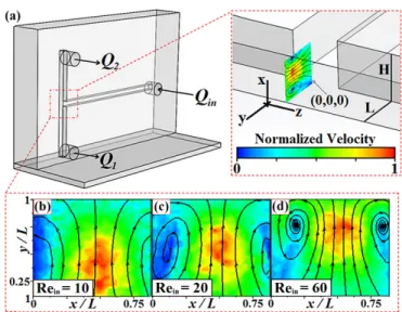
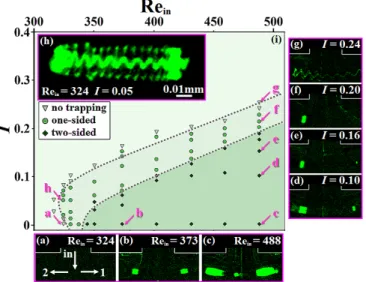
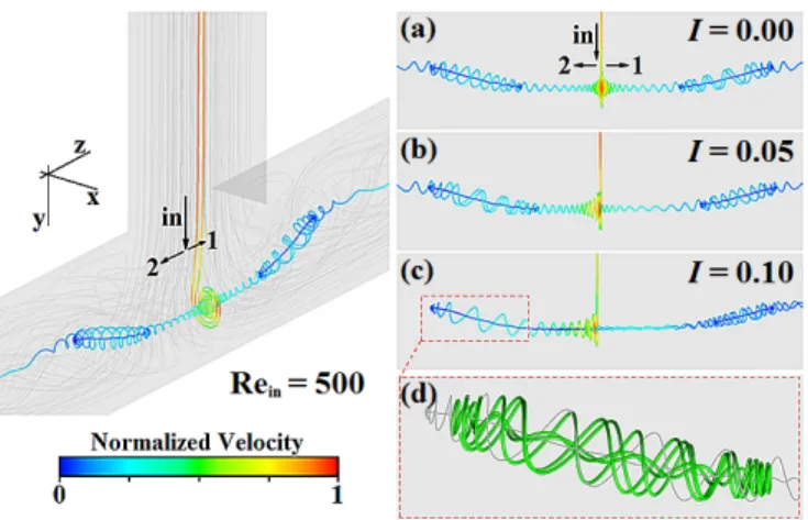
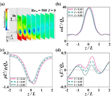
Microscopic investigation of vortex breakdown in a dividing T-junction flow
9
0
0
全文
(2)
(3)
(4)
(5)
(6)
(7)
(8)
(9)
図
関連したドキュメント
2 Combining the lemma 5.4 with the main theorem of [SW1], we immediately obtain the following corollary.. Corollary 5.5 Let l > 3 be
It is suggested by our method that most of the quadratic algebras for all St¨ ackel equivalence classes of 3D second order quantum superintegrable systems on conformally flat
Compactly supported vortex pairs interact in a way such that the intensity of the interaction decays with the inverse of the square of the distance between them. Hence, vortex
We present sufficient conditions for the existence of solutions to Neu- mann and periodic boundary-value problems for some class of quasilinear ordinary differential equations.. We
The author, with the aid of an equivalent integral equation, proved the existence and uniqueness of the classical solution for a mixed problem with an integral condition for
Later, in [1], the research proceeded with the asymptotic behavior of solutions of the incompressible 2D Euler equations on a bounded domain with a finite num- ber of holes,
“Breuil-M´ezard conjecture and modularity lifting for potentially semistable deformations after
Then it follows immediately from a suitable version of “Hensel’s Lemma” [cf., e.g., the argument of [4], Lemma 2.1] that S may be obtained, as the notation suggests, as the m A
