Overlapping Domain Decomposition with Non-matching Grids(Domain Decomposition Methods and Related Topics)

Overlapping

Domain Decomposition with

Non-matching

Grids

-Yuri

A. Kuznetsov

Institute of Numerical $\mathrm{M}\mathrm{a}\mathrm{t}\mathrm{h}\mathrm{e}\mathrm{m}.\mathrm{a}\mathrm{t}\mathrm{i}_{\mathrm{C}}\mathrm{s}$

Russian Academy of Sciences, Moscow

Abstract –A macro-hybrid formulation based on overlapping domain

decompo-sition is introduced and studied for a model elliptic partial differential equation.

The problem is discretized by the mortar element method using non-matching grids

on the interfaces between subdomains. An iterative method of an optimal order of arithmetical complexity is proposed for solving the arising algebraic systems in the

case of regular quasiuniform hierarchical grids. Results of numerical experiments

are presented.

1

INTRODUCTION

In this paper we consider two topics. In Section 2 we introduce a new macro-hybrid

formulation for the Poisson equation with the Neumann boundary condition based on

overlapping domain decomposition. An example of such$\mathrm{f}\mathrm{o}\mathrm{r}\acute{\mathrm{m}}\mathrm{u}\mathrm{l}\mathrm{a}\mathrm{t}\mathrm{i}_{\mathrm{o}\mathrm{n}}$

was originally given

in [8]. The approach proposed here has many common points with the decentralization

methods studied more than twenty years ago in $[1, 10]$. In these papers the authors

used splittings ofbilinear forms between different subdomains to decompose avariational

problem.

The second important topic is presented in Section 4 where we consider an extension

of results from $[7, 8]$ to the case of overlapping subdomains. Here we present several

results which mainly concern the construction of the interface preconditioner.

In

Section

5 results ofnumerical experiments for a $2\mathrm{D}$ test problem are given.

2

MACRO-HYBRID BASED

ON OVERLAPPING

DOMAIN

DECOMPOSITION

Let us consider a model elliptic problem

$-\Delta u+Cu$ $=$ $f$

in

$\Omega$

$\frac{\partial u}{\partial \mathrm{n}}$ $=0$ on $\partial\Omega$

(1)

where $f\in L_{2}(\Omega)$ is a given function, $c\equiv \mathrm{c}\mathrm{o}\mathrm{n}\mathrm{s}\mathrm{t}\in(0;1$], $\partial\Omega$ is the boundary of a domain

$\Omega$ and

$\Omega$ is a polygon in $\mathrm{R}^{2}$, with diam

$(\Omega)\sim O(1)$, and all further subdomains of $\Omega$

a.re

also

polygons with diameters $O(1)$

.

The classical weak formulation of (1) is: find $u\in H^{1}(\Omega)$ such that

$\Phi(u)=$ $\min\Phi(v)$, (2)

$v\in H^{1}(\Omega)$

where

$\Phi(v)=\int\Omega[|\nabla v|2+Cv^{2}-2fv]d\Omega$. (3)

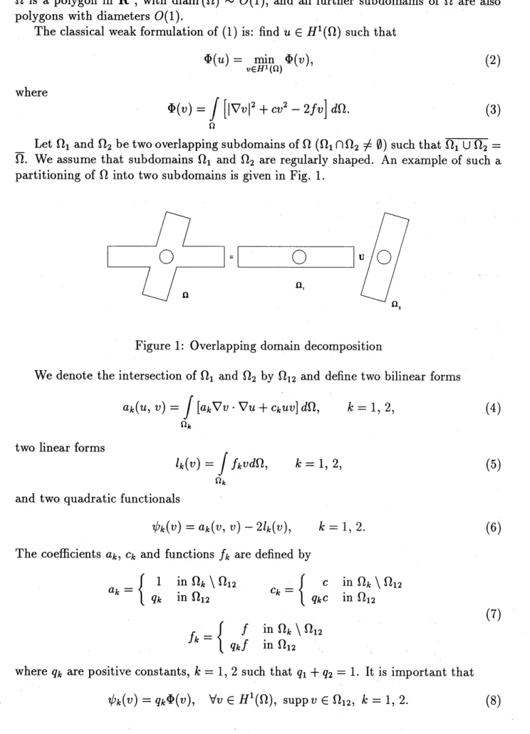
Let $\Omega_{1}$ and $\Omega_{2}$ be twooverlapping subdomains of_{$\Omega(\Omega_{1}\cap\Omega_{2}\neq\emptyset)$} such that $\overline{\Omega_{1}\cup\Omega_{2}}=$

$\overline{\Omega}$

.

We assume that subdomains $\Omega_{1}$ and $\Omega_{2}$ are regularly shaped. An example of such a

partitioning of$\Omega$ into two subdomains is given in Fig. 1.

Figure 1: Overlapping domain decomposition

We denote the intersection of$\Omega_{1}$ and $\Omega_{2}$ by $\Omega_{12}$ and define two bilinear forms

$a_{k}(u, v)= \int[ak\Omega_{k}\nabla v\cdot\nabla u+C_{k}uv]d\Omega$, $k=1,2$, (4)

two linear forms

$l_{k}(v)= \Omega\int_{k}fkvd\Omega$, $k=1,2$, (5)

and two quadratic functionals

$\psi_{k}(v)=a_{k}(v, v)-2l_{k}(v)$, $k=1,2$. (6)

The coefficients $a_{k},$ $c_{k}$ and functions $f_{k}$ are defined by

$a_{k}=\{$ 1 in $\Omega_{k}\backslash \Omega_{12}$ $q_{k}$ in $\Omega_{12}$ $c_{k}=\{$ $c$ in $\Omega_{k}\backslash \Omega_{12}$ $q_{k^{C}}$ in $\Omega_{12}$ $f_{k}=\{$ (7) $f$ in $\Omega_{k}\backslash \dot{\Omega}_{12}$ $q_{k}f$ in $\Omega_{12}$

where $q_{k}$ are positive constants, $k=1,2$ such that $q_{1}+q_{2}=1$

.

It is important that

To introduce andto analyze macro-hybridformulationsof elliptic

_moblems

wehave to deal$\mathrm{w}\mathrm{i}\dot{\mathrm{t}}\mathrm{h}$

interfaces betweensubdomains. Tothis end weintroducethefollowingnotation:

$\Gamma_{k}$ _$=$ $(\partial\Omega_{k}\cap\Omega)$, $k=1,2$, (9)

$\Gamma$ _$=$ $\Gamma_{1}\cup\Gamma_{2}$.

Now we introduce the space $V=H^{1}(\Omega_{1})\cross H^{1}(\Omega_{2})$

,

the space

$W= \{\overline{v}=(v_{1}, v_{2}):\overline{v}\in V,\int_{\Gamma}(v_{1}-v_{2})\mu dS=0,$ $\forall\mu\in H-1/2(\Gamma)\}$ (10)

and the $..\mathrm{q}_{l}\mathrm{u}\mathrm{a}\mathrm{d}\mathrm{r}\mathrm{a}\mathrm{t}\mathrm{i}\mathrm{C}\mathrm{f}\mathrm{u}\mathrm{n}\mathrm{c}\mathrm{t}\mathrm{i}\mathrm{o}\mathrm{n}\mathrm{a}:1.-$

$\psi(\overline{v})=\psi_{1}(v_{\iota})+^{\psi}2(v_{2})$, $\overline{v}\in V$. (11)

It can be shown (see, for instance [5]) that under the assumptions made the following

macro-hybrid formulation of problem (1):

$\overline{u}\in V$ :

$\psi(\overline{u})=\min_{\overline{v}\in W}\psi(\overline{v})$ (12)

has a unique solution and is equivalent to problem (2). We understand the equivalence

in the sense that

$u(x)=u_{k}(x)$ $\forall x\in\Omega_{k}$, (13)

where $u$ is the solution function to (2).

Problem (12) has also an equivalent formulation in terms of Lagrangemultipliers. For

instance, in the case $0\dot{\mathrm{f}}$example in Fig. lb it can be presented in the following form: find

$(\overline{u},\overline{\lambda})\in V\cross$ A such that

$a_{1}(u_{1,1}v)+ \int_{1}\lambda 1v_{1}ds-\int_{\Gamma\Gamma 2}\lambda 2v1ds$ $=$ $l_{1}(v_{1})$,

$a_{2}(u_{2}, v_{2})- \Gamma_{1}\int\lambda_{1}v2dS+\int_{\Gamma_{2}}\lambda_{2}v2d_{S}$ $=$ $l_{2}(v_{2})$, $\int(u_{1}-u_{2})\mu 1dS$ $–0$,

(14)

$\int_{\Gamma_{2}}^{\Gamma_{1}}(u_{1}-u2)\mu_{2}dS$ $=$ $0$,

$\forall(\overline{v},\overline{\mu})\in V\cross\Lambda$

.

Here $\Lambda=\prod_{s=1}^{2}H-1/2(\Gamma_{S})$. It can be easily shown that

$\lambda_{1}=-q_{1^{\frac{\partial u_{1}}{\partial \mathrm{n}_{1}}}}$ on $\Gamma_{1}$, $\lambda_{2}=-q_{2^{\frac{\partial u_{2}}{\partial \mathrm{n}_{2}}}}$ on $\Gamma_{2}$, (15)

where $\mathrm{n}_{1}$ and $\mathrm{n}_{2}$ are the outer normal

$.\mathrm{v}$

ecto.rs

to

$\partial\Omega_{1}$

. and

$\partial\Omega_{2}$, respectively. Recall that

$u_{1}\equiv u$ in $\Omega_{1}$ and _{$u_{2}\equiv u$} in $\Omega_{2}$.

In a compact form (14) can be presented $[6^{\backslash },‘ 5]$

by: find $(\overline{u},\overline{\lambda})\in V\cross\Lambda$ such that

\^a$(\overline{u},\overline{v})+b(\overline{\lambda},\overline{v})$ _$=$ $l(\overline{v})\wedge$,

(16)

Here

$V= \prod_{k=1}V_{k}2$

,

$V_{k}=H^{1}(\Omega_{k}),$ $k_{--}1,2$,

$\Lambda=\prod_{s=1}^{2}..\Lambda_{s}$, _{$\Lambda_{S^{--H^{-1}}}/2(\mathrm{r}_{s}),$} $s=1,2$, (17)

\^a$( \overline{u},\overline{v})=\sum_{k=1}^{2}a_{k}(u, v)$, $l( \overline{v})\wedge=\sum_{k=1}^{2}l_{k(v})$.

Remark If$\int_{\Omega}fd\Omega=0$ and $c\ll 1$ then problem (1) can be considered as a singular

perturbation of the

Neumann

problem

$-\Delta u$ $=$ $f$ in $\Omega$

$\frac{\partial u}{\partial \mathrm{n}}$

$=$ $0$ on $\partial\Omega$

.

(18)

3

THE MORTAR

ELEMENT METHOD

AND

ALGEBRAIC SYSTEMS

We consider the only case when $\Omega_{kh}$ are conforming triangular partitions of$\Omega_{k},$ $k=1,2$.

Then $V_{kh}$ are the standard piece-wide linear finite element subspaces of $V_{k}\equiv H^{1}(\Omega_{k})$,

$k=1,2$

.

The finite element subspaces $\Lambda_{sh}\subset\Lambda\equiv H^{-\frac{1}{2}}(\Gamma_{s}),$ $S=1,2$ are chosen using the

mortar element technique $i^{\mathrm{f}\mathrm{r}\mathrm{o}\mathrm{m}}[3,2,8]$.

The mortar finite element discretization of (16)$-(17)$ is defined by: find $(\overline{u}_{h},\overline{\lambda}_{h})\subset$

$V_{h}\cross\Lambda_{h}$ such that

$b(^{\frac{\overline{u}}{\mu}},\overline{u}_{h}’)\hat{a}(h\overline{v})+b(\overline{\lambda}h,\overline{u}h)$ $==$ $0l(,\overline{v})\wedge$, (19)

V$(\overline{v},\overline{\mu})\in V_{h}\cross\Lambda_{h}$ where $\Lambda_{h}=\prod_{s=1}^{2}\Lambda_{sh}$. Problem (19) leads to an algebraic system

$Ax=y$ (20)

with a saddle-point matrix

$A=$

(21)

and vectors

$x=$

,

$y=$

.

(22)

Here $A$ is a symmetric positive definite matrix and $\mathrm{k}\mathrm{e}\mathrm{r}BT^{-}=0$. It

follows immediately that $\det A\neq 0$.

For further analysis we need a more detailed description of $A$ and $B$ in block forms.

The simplest block representations of $A$ and $B^{T}$ are:

Here the $k\mathrm{t}\mathrm{h}$ block corresponds

to the degrees of freedom of the finite element space $V_{k,h}$,

$k=1,2$

.

For each subdomain $\Omega_{k}$ we partitiondegrees of freedom ($\mathrm{g}\mathrm{r}\mathrm{i}\acute{\mathrm{d}}$nodes) into two groups.

In the second group denoted by $\Gamma$ we collect the degrees

offreedom which correspond to

the grid nodes belonging to $\Gamma$

.

All

other degrees of freedom we collect in the first group

denoted by $I$

.

These partitionings induce the

following

blockrepresentations:

$A_{k}=$

, $B_{k}^{T}=$

.

(24)

Let $B$ be a symmetric positive definite matrix and $\mathcal{H}=B^{-1}$. Since _$A=A^{T}$ the

preconditioned Lanczos $[11, 8]$ can be used to solve system (20). In this paper we _also

recommend the preconditioned $\mathrm{c}\mathrm{o}\mathrm{n}\mathrm{j}.\mathrm{u}\mathrm{g}\mathrm{a}\mathrm{t}\mathrm{e}$ method based on the

$B$-norm of minimal

er-rors [11]: $\hat{p}\iota$ _$=$ $\{$ $\mathcal{H}\xi^{0}$, $l=1$, $\mathcal{H}\xi^{l-1}-\alpha\iota\hat{p}\iota-1$, $l>1$, $p_{l}$ $=$ $\mathcal{H}A\hat{p}\iota$, (25) $x^{l}$ $=$ $x^{l-1}-\beta lpl$, $\alpha_{l}=\frac{(\xi^{l-}1A\hat{p}\iota-1)_{\mathcal{H}}}{(A\hat{p}\iota-1,A\hat{p}\iota_{-}1)_{\mathcal{H}}},$, $\beta_{l}=\frac{(\xi^{l-1},\hat{p}l)}{(A\hat{p}_{l},A\hat{p}l)\mathcal{H}}$,

where $\xi^{l}=Ax^{l}-y$ are the residual _{vectors, $l=1,2,$}

$\ldots$ Assume that the eigenvalues

of$\mathcal{H}A$ belong to the union of segments

$[d_{1} ; d_{2}]$ and $[d_{3};d_{4}]$ with _{$d_{1}\leq d_{2}<0<d_{3}\leq d_{4}$}

.

Then the convergence estimate

$||x^{\iota_{-x}}||_{\mathcal{H}}\leq 2q^{l}||X^{0}-x||_{\mathcal{H}}$, _{$l\geq 1$}, (26)

holds [11] where $q= \frac{\hat{d}-\check{d}}{\hat{d}+\check{d}},\hat{d}=\max\{d_{4};|d_{1}|\}$, and _{$\check{d}=\min\{d_{3};|d_{2}|\}$}.

4

BLOCK

DIAGONAL

_{PRECONDITIONER}

We propose a preconditioner $\mathcal{H}$ as a block diagonal

matrix:

$\mathcal{H}=$ (27)

where $H_{A}$ is also a block diagonal matrix:

$H_{A}=$

. (28)

All blocks are symmetric positive definite matrices. $H_{k}$ are said to be the subdomain

If matrices $H_{k}$ are spectrally equivalent to the matrices $A_{k}^{-1}$ with constants

indepen-dent of the value of the coefficient $c$, and if a matrix $H_{\lambda}$ is spectrally equivalent to the

matrix $S_{\lambda}^{-1}$ with $S_{\lambda}$ given by

$S_{\lambda}=BA-1BT \equiv\sum_{k=1}^{2}Bk\mathrm{r}s_{k}^{-1\tau_{\mathrm{r}}}\mathrm{r}Bk$ (29)

with the constants independent of the value of$c$then the values of$\hat{d},\check{d}$in (26) are positive

constants [7] also independent of $c$. Here

$s_{k\mathrm{r}}=A_{k\Gamma}-Ak\Gamma IA^{-}kI1A_{k}I\Gamma$ (30)

are the Schur complements. Our aim is to construct a preconditioner $\mathcal{H}$spectrally

equiv-alent [7] to the matrix $A^{-1}$ with constants independent of

$c$.

4.1

_{Subdomain Preconditioners}

Let us define matrices $[mathring]_{k}_{A}$

and $M_{k}$ by:

$([mathring]_{k}_{A}v, w)$

$= \int_{\Omega_{k}}\nabla v_{h}\cdot\nabla w_{h}d\Omega$, (31)

$(M_{k}v, w)$

$= \int_{\Omega_{k}}v_{h}w_{h}d\Omega$

$\forall v_{h},$_{$w_{h}\in V_{kh},$} $k=1,2$. Thus, matrices $A_{k}\mathrm{o}$

are the stiffness matrices forthe $\mathrm{o}\mathrm{p}\mathrm{e}\mathrm{r}\mathrm{a}\mathrm{t}\mathrm{o}\mathrm{r}-\triangle$

with the Neumann boundary conditions, and $M_{k}$ are the corresponding mass matrices. It

can be easily shown [8] that

$A_{k}^{-1} \sim(\mathrm{O}A_{k}+Mk)-1+\frac{1}{c}P_{k}$ (32)

where$P_{k}$ is the $M_{k}$-orthogonal projector onto$\mathrm{k}_{\mathrm{e}\mathrm{r}}Ak\mathrm{o}$

and thesign $”\sim$” denotesthe spectral

equivalence. Moreover, the constants of the spectral equivalence in (32) are independent

of the value of $c$

.

Suppose that a matrix $H_{k}\mathrm{o}$ is

spectrally equivalent to the matrix $([mathring]_{k}_{A}+M_{k})^{-1}$ Then

the matrix

$H_{k}=[mathring]_{k}_{H}+ \frac{1}{c}P_{k}$ (33)

is spectrally equivalent to matrix $A_{k}^{-1}$ with constants independent of the value of

$c$.

We have plenty of choices for $H_{k}^{\mathrm{o}},$

$k=1,2$.

4.2

Interface

Preconditioner

We can easily shown [8] that

$S_{\Gamma k}^{-1} \sim\tilde{S}^{-1}+k\frac{1}{c}P\mathrm{r}k$

where

$\tilde{S}_{k}^{-1}$ isthe Schurcomplementforthematrix $A_{k}\mathrm{o}+M_{k}$ and $P_{\Gamma k}$ isthe $M_{\Gamma k}$orthogonal

projector onto $\mathrm{k}\mathrm{e}\mathrm{r}S_{\Gamma k}$ in the case $c=0$

.

Moreover, the constants of equivalence in (34)

are independent ofthe value of$c$

.

Here $M_{\Gamma k}$ is the interfacemass matrix defined by:

$(M_{\Gamma k}v, w)$

$= \int_{\mathrm{r}_{k}}v_{h}w_{h}d_{S}$ V$v_{h},$

$w_{h}\in V_{k}\mathrm{r}h$ (35)

where $V_{k\Gamma h}$ is the trace of $V_{kh}$ into $\Gamma_{k},$ $k=1,$

$\ldots,$ $m$.

Let the matrices

$H_{k}^{\mathrm{o}}=($ $[mathring]_{k\Gamma}_{H}IH_{k}^{\mathrm{O}}I$ $H^{\mathrm{O}}kIH^{\mathrm{o}}k\mathrm{r}\mathrm{r}$

)

(36)

be spectrally equivalent to the matrices $(\mathrm{O}A_{k}+M_{k})^{-1},k=1,2$. We can also prove that

the matrix

$\hat{S}_{\lambda}=\sum_{=k1}^{2}Bk\Gamma([mathring]_{k}_{H}\Gamma+\frac{1}{c}P\mathrm{r}k)B_{k}^{\tau_{\Gamma}}$ (37)

is spectrally equivalent to $S_{\lambda}$ with constants independent ofthe value of _$c$

.

To construct the interface preconditioner $H_{\lambda}$ we shall use the preconditioned

Cheby-shev iterative procedure $[4, 7]$

.

Let $\hat{H}_{\lambda}$

be a symmetric positive defined matrix and

$\nu_{\lambda}=\lambda_{\max}/\lambda_{\min}$ where $\lambda_{\max}$ and $\lambda_{\min}$ are the maximal and minimal eigenvalues of $\hat{H}_{\lambda}\hat{S}_{\lambda}$

,

respectively. Then for any $t_{\lambda}\sim\sqrt{\nu_{\lambda}}$ the matrix

$H_{\lambda}=[I_{\lambda}-\square (I_{\lambda}-\alpha_{t}\hat{H}\lambda\hat{s}_{\lambda})t=1t_{\lambda}]\hat{s}^{-1}\lambda$ (38)

is spectrally equivalent to the matrix $S_{\lambda}^{-1}$

.

Let $\hat{B}_{\lambda}$ be a symmetric positive

definite matrix such that $1 \in[\mu\min;\mu_{\max}]$ where $\mu\min$

and $\mu_{\max}$ are the minimal and maximal eigenvalues of the matrix $\hat{B}_{\lambda}^{-1}\sum_{1k=}^{2}B_{k\mathrm{r}}H_{k\Gamma}B_{k\Gamma}^{T}$,

respectively. Then for the choice $\hat{H}_{\lambda}=\hat{R}_{\lambda}^{-1}$ where

$\hat{R}_{\lambda}=\hat{B}_{\lambda}+\frac{1}{c}k\sum_{=1}Bk\mathrm{r}P2k\mathrm{r}B^{T}k\Gamma$

’ (39)

the estimate

$\nu_{\lambda}\leq\hat{\nu}_{\lambda}\equiv\mu_{\max}/\mu\min$ (40)

holds.

A solution algorithm for a system

$\hat{R}_{\lambda^{Z}}=g$

is presentedin $[8, 9]$. It includes a so called “coarse grid” problembased on the projectors

4.3

Arithmetical

Complexity for

Hierarchical grids

Assume that grids $\Omega_{kh}$ are regular, quasiuniform and hierarchical with the average grid

step size $h\sim\sqrt[\mathrm{p}]{N}$where _$N$ is the dimension of matrix _$A$.

In this case we can usevarious $V$-cycle multilevelpreconditioners to define matrix $[mathring]_{k}_{H}$

in (33). These preconditioners are spectrally equivalent to the matrices $(A_{k}^{\mathrm{o}}+M_{k})^{-1},$ _$k=$

$1,2$ andhave theoptimalorder of arithmetical complexity $[12, 13]$, $\mathrm{i}$

.

$\mathrm{e}$. the multiplication

with such a preconditioner by a vector costs $O(N)$ arithmetical operations.

Our choice $H_{k\Gamma}^{\circ}$

in (37) as the corresponding blocks of $V$-cycle multilevel

precon-ditioner (BPX or MDS-type) is based on two observations. The first one is obvious:

spectral equivalenceof $H_{k\Gamma}^{\mathrm{o}}$

and $\tilde{S}_{\Gamma k}^{-1}$ follows directly from the spectral equivalence

of $H_{k}$

and $(\mathrm{O}A_{k}+M_{k})^{-1},k=1,2$

.

The second observation is rather technical and _concerns

im-plementation algorithms for $V$-cycle multilevel preconditioners: multiplication of $[mathring]_{k\Gamma}_{H}$

by

a vector can be implemented with $O(h^{-1})$ arithmeticaloperations. The latter observation

has at least one very important consequence: the corresponding matrix $\hat{S}_{\lambda}$ can be

multi-plied by a vector with $O(h^{-1})$ arithmeticaloperations, i.e. multiplication with $\hat{S}_{\lambda}$ has

the

optimal order of arithmetical complexity.

$\mathrm{s}$

It remains to choose preconditioner$R_{\lambda}$, and wedo not need an optimal preconditioner

because the dimension of $S_{\lambda}$ is much smaller than the dimension of$A$.

In paper [7] we proposed to choose $\hat{B}_{\lambda}$

being equal to a scalar matrix which is a

spectrally equivalent to the matrix $\sum_{k=1}^{2}B_{k\mathrm{r}\mathrm{r}}M_{k}^{-1}B^{T}k\Gamma$. With this choice, obviously

$\nu_{\lambda}\leq \mathrm{c}\mathrm{o}\mathrm{n}\mathrm{s}\mathrm{t}\cdot h^{-2}$

where the constant is independent of$h$ and _$c$, and the multiplication $B_{\lambda}^{-1}$ by a vector can

be implemented with $O(h^{-1})$ arithmetical operations.

On the basis of thelatter facts we conclude that $t_{\nu}$ should be proportional to $h^{-1}$, and

arithmetical complexity of the corresponding preconditioner $H_{\lambda}$ in (38) is of the order

$O(h^{-1})$

.

In some particular cases we can prove _{$[4, 7]$} that $t_{\nu}\sim h^{-1/2}$ and consequently

5

NUMERICAL EXPERIMENT

The numericalexperiments have been performed

_for..

the test case given in Fig. 2.

$\mathrm{r}4_{\mathrm{h}}$

.

Figure 2:

Cartesian

locally fitted grids in $\Omega_{1}$ and $\Omega_{2}$

In the subdomains $\Omega_{1}$ and $\Omega_{2}$ we use rectangular cartesian grids which are fitted to

the interface boundary which consists of four straight segments. These grids are givenin

Fig. 2.

Table 1: Results of numerical experiments

Cartesian

Cartesian

Number of Number of

grids in $\Omega_{1}$ grids in $\Omega_{2}$ Chebyshev Lanczos

iterations iterations $16\cross 8$ $16\cross 8$ 14 44 $32\cross 16$ $32\cross 16$ 23 52 $64\cross 32$ $64\cross 32$ 32 52 $128\cross 64$ 128 $\cross 64$ 45 54 $256\cross 128$ $256\cross 128$ 63 55

Remark For numerical experiments the subdomain BPX preconditioners were used

in combination with the fictitious domain technique, because grids $\Omega_{kh},$ $k=1,2$ aren’t

hierarchical. The procedure of coupling is described in [7].

ACKNOWLEDGEMENTS

The results of numerical experiments in Section 5 are kindly given for this paper by

References

[1] Bensoussan A., Lions J.-L., and TemamR. (1974) Surles methodes de decomposition,

de decentralisation et de coordination et applications. In Lions J.-L. and Marchuk

G. I. (eds) Methodes Mathematiques de L’Informatique-4, pages

133-257.

Dunod,

Paris.

[2] Ben Belgacem F. B. and Maday Y. (1994) The mortar element method for three

dimensional finite elements. Technical report, Universite Paul Sabartier.

[3] Bernardi C., Maday Y., and Patera A. (1989) A new nonconforming approach to

domain decomposition: the mortar element method. In Lions J.-L. and Bresis H.

(eds) Nonlinear PDE and their Applications. Pitman.

[4] Bramble J., Pasciak J., and SchatzA. (1986) The construction of preconditioners for

elliptic problems by substructuring, 1. Math. Comp.

47:

103-134.

[5] Brezzi F. and FortinM. (1991) Mixedand Hybrid Finite Element Methods.

Springer-Verlag, New York.

[6] Glowinski R. andWheelerM. (1988) Domain decomposition and mixedfiniteelement

methods for elliptic problems. In Glowinski R., Golub G., G.Meurant, and Periaux

J. (eds) Proc. First DDInt. Conf., pages

144-172.

SIAM, Philadelphia.

[7] Kuznetsov Y. A. (1995) Efficient iterative solvers for elliptic finite element problems

on nonmatching grids. Russ. J. Numer. Anal. Math. Modelling 10:

187-211.

[8] Kuznetsov Y. A. (June 1995) Iterative solvers for elliptic finite element problems

on nonmatching grids. In Proc. Int. $Co\check{n}f$. AMCA-95, pages 64-76. NCC Publisher,

Novosibirsk.

[9] Kuznetsov Y. and Wheeler M. (1995) Optimal order substructuring preconditioners

for mixed finite element methods on nonmatching grids. East-West J. Numer. Math.

3:

127-143.

[10] Lemonnier P. (1974) Resolution numerique d’equations aux derivees partielles par

decomposition et coordination. In Lions J.-L. and Marchuk G. I. (eds) Methodes

Mathematiques de L’Informatique-4, pages

259-299.

Dunod, Paris.

[11] Marchuk G. I. and Kuznetsov Y. A. (1974) Methodes iteratives et fonctionnelles

quadratiques. In Lions J.-L. and Marchuk G. I. (eds) Methodes Mathematiques de

L’Informatique-4. Dunod, Paris.

[12] Oswald P. (1994) Multilevel Finite Element Approximations: Theory and

Applica-tions. Teubner-Scripten zur Numerik.

[13] Xu J. (1992) Iterative methods by space decomposition and subspace correction.