Zoom Factor Compensation for Monocular SLAM
3
0
0
全文
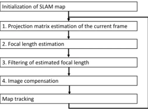
(2) Zoom Factor Compensation for Monocular SLAM Takafumi Taketomi∗. Janne Heikkila¨ †. Nara Institute of Science and Technology. University of Oulu. Remove camera zooming effect. Initialization of SLAM map 1. Projection matrix estimation of the current frame 2. Focal length estimation 3. Filtering of estimated focal length. Input image. Compensated image. 4. Image compensation. Figure 1: Image compensation for removing the camera zooming effect. The left image is an input image. The right image is an compensated image by using the estimated focal length change.. A BSTRACT SLAM algorithms are widely used in augmented reality applications for registering virtual objects. Most SLAM algorithms estimate camera poses and 3D positions of feature points using known intrinsic camera parameters that are calibrated and fixed in advance. This assumption means that the algorithm does not allow changing the intrinsic camera parameters during runtime. We propose a method for handling focal length changes in the SLAM algorithm. Our method is designed as a pre-processing step for the SLAM algorithm input. In our method, the change of the focal length is estimated before the tracking process of the SLAM algorithm. Camera zooming effects in the input camera images are compensated for by using the estimated focal length change. By using our method, camera zooming can be used in the existing SLAM algorithms such as PTAM [4] with minor modifications. In the experiment, the effectiveness of the proposed method was quantitatively evaluated. The results indicate that the method can successfully deal with abrupt changes of the camera focal length. Index Terms: H.5.1 [Multimedia Information Systems]: Artificial, augmented, and virtual realities—; I.4.1 [Digitization and Image Capture]: Imaging geometry— 1 I NTRODUCTION In this paper, we propose a method for handling the focal length change caused by camera zooming in the SLAM algorithm. The proposed method is designed as a preprocessing step of the SLAM algorithm. In our method, the focal length change is estimated using 2D-3D correspondences in the current image and the projection matrices of the keyframes. The camera zooming effect in the current image is compensated for by using the estimated focal length change, as shown in Fig. 1. By using the proposed preprocessing method, the existing SLAM algorithms can handle camera zooming. Many SLAM algorithms have been proposed in the AR and computer vision research fields [2, 4, 3]. Most SLAM algorithms are composed of separate tracking and mapping processes. In the tracking process, natural features are tracked in successive frames. 2D3D correspondences of tracked natural features are used for estimat∗ E-mail: † E-mail:. [email protected] [email protected]. Map tracking. Figure 2: Flow diagram of the proposed method.. ing the current camera pose. On the other hand, the mapping process is executed for estimating 3D positions of natural features by triangulation using intrinsic camera parameters and 2D correspondences of natural features in multiple keyframes. In most methods, estimated 3D positions of natural features and camera poses of the keyframes are optimized after triangulation. In this process, most SLAM algorithms assume the known intrinsic camera parameters. Civera et al. proposed a self-calibration method for the SLAM algorithm [1]. In this method, intrinsic camera parameters are estimated during the SLAM process. Although this method can be used for an unknown intrinsic camera parameter case, the method still assumes fixed parameters. To the best of our knowledge, a SLAM algorithm which can deal with focal length changes has not been proposed until now. 2. R EMOVING T HE C AMERA Z OOMING E FFECT. In this study, we propose a method for dealing with camera zooming in SLAM algorithms. The method is composed of four parts, as shown in Fig. 2. First, a projection matrix of the current frame is obtained, and the focal length ratio between a current frame and the first keyframe is obtained. The estimated focal length ratio is then filtered for achieving more stable result. Finally, camera zooming effects in the input camera images are compensated for by using the estimated focal length ratio. The focal length change estimation process is based on the method described in [5]. In this method, focal lengths of each image are estimated from projection matrices of the cameras. We extended this method to achieve sequential focal length estimation. In our approach, firstly, the projection matrix of the current frame is estimated using tracked natural features. The focal length change is determined based on the estimated projection matrix and the projection matrices of the keyframes. First, the keyframes that have been used for determining 3D positions of tracked natural features are selected from the map. In addition, the first keyframe which is used for initialization is always selected to provide the reference focal length. The relationship between intrinsic camera parameters and projection matrices of the selected keyframes and the current frame can be described as follows: fi2 0 0 T K iK i = 0 (1) fi2 0 = M i Ω∗ M Ti 0 0 1.
(3) f1,t =. f1 ft. (2). The focal length estimation process is sensitive to estimation errors of the projection matrices. In order to achieve stable focal length ratio, we employ two filtering processes: median filtering for robust estimation and temporal filtering for smoothing. Median Filtering for Robust Focal Length Estimation: In the focal length estimation process, the zoom factor between the first keyframe and the current frame f1,t is estimated, together with focal length ratios between other keyframes and the current frame f2,t , f3,t , . . . , fn,t (n represents the number of selected keyframes). In addition, zoom factors between the first keyframe and the other keyframes f1,2 , f1,3 , . . . , f1,n have already been estimated for the previous time steps. By using these values, we can obtain candidates of the zoom factor between the first keyframe and the current frame as follows: f1,t , f1,2 f2,t , f1,3 f3,t , . . . , f1,n fn,t. (3). The median value of these candidates is selected as the zoom factor between the first keyframe and the current frame f1,t . Temporal Filtering for Smoothing: Estimated zoom factor involves estimation error. In order to suppress the noise effect, in the proposed method, we employ temporal filtering for smoothing the estimate. The estimated zoom factor is filtered by the following equation. fˆ1,t = α f1,t + (1 − α) fˆ1,t−1 (4) where fˆ represents a filtered zoom factor and α represents a coefficient for smoothing. The zoom factor can change in successive frames. In order to tolerate smooth changes, we use one of the following criteria for accepting the estimation result.
(4)
(5) •
(6) f1,t − fˆ1,t−1 < ε1
(7) : Estimated focal length ratio of the current frame should be similar to that of the filtered previous value.
(8)
(9) •
(10) f1,t − f1,t−1 < ε2
(11) : Similar focal length ratios are estimated in the current and previous frames.
(12)
(13) •
(14) f 0 1,t − f 0 1,t−1 < ε3
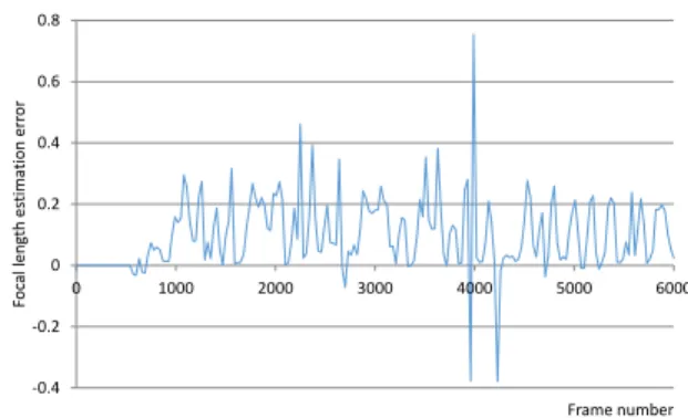
(15) : Gradients of estimated focal lengths are similar. Gradients are calculated by f 0 1,t = f1,t − f1,t−1 , f 0 1,t−1 = f1,t−1 − f1,t−2 . The second and third conditions are for detecting the focal length change. If the estimated zoom factor ft satisfies one or more conditions, f1,t is accepted and used in the filtering process. If all conditions are false, the zoom factor of the previous frame is used as an input to the filtering process f1,t = fˆ1,t−1 . Finally, the input image is scaled using the filtered zoom factor fˆ1,t . 3 E XPERIMENT To demonstrate the effectiveness of the proposed method, the accuracy of focal length estimation was quantitatively evaluated. In the experiment, we used PTAM [4] as an existing SLAM algorithm. In the experiment, the hardware included a desktop PC (CPU: Corei53570 3.4 GHz, Memory: 8.00 GB) and a Sony NEX-VG900 video camera, which records 640 × 480 pixel images with an optical zoom lens (Sony SEL1018, f = 10mm − 18mm).. 0.8 0.6 Focal length estimation error. where K is the intrinsic camera parameter matrix, Ω∗ is the absolute quadric, f is the focal length, and M is the projection matrix. Ω∗ has the 4 × 4 matrix structure and it has scale ambiguity. Therefore, intrinsic camera parameter matrices K i and the absolute quadric Ω∗ can be calculated using the rank 3 constraint [5]. Camera zoom factor is the focal length ratio f1,t between focal lengths of the first keyframe f1 and the current frame ft as follows:. 0.4 0.2. 0 0. 1000. 2000. 3000. 4000. 5000. 6000. -0.2 -0.4 Frame number. Figure 3: Focal length estimation error in each frame.. In the video sequence, the camera moves freely in the real environment, which includes translation, rotation, and camera zooming. In order to evaluate the accuracy of focal length estimation, reference focal length values for each image were obtained by an offline reconstruction method [6, 7]. The reference values were obtained at every 30th frames. Fig. 3 shows the result of zoom factor estimation errors in each frame. An average error for focal length estimation was 0.113 and its standard deviation was 0.109. The result confirms that the proposed method can estimate the zoom factor change with reasonable accuracy. The execution time for our preprocessing algorithm was 12 ms, and the overall execution time for the online tracking process was 26 ms. This proves that the proposed method can work in realtime. 4 C ONCLUSION In this paper, we proposed a zoom factor compensation method for dealing with camera zooming in SLAM algorithms. By using our method, the camera zooming effect in the input image is normalized with respect to the first keyframe before the tracking process. In order to estimate the focal length change, we developed an online focal length estimation framework. In this framework, the estimated focal length is filtered to achieve more stable result. The effectiveness of the proposed method was demonstrated in the experiments. R EFERENCES [1] J. Civera, D. R. Bueno, A. Davison, and J. M. M. Montiel. Camera self-calibration for sequential bayesian structure from motion. In Proc. ICRA, pages 403–408, 2009. [2] A. Davison, W. Mayol, and D. Murray. Real-time localization and mapping with wearable active vision. Proc. ISMAR, pages 18–27, 2003. [3] C. Forster, M. Pizzoli, and D. Scaramuzza. SVO: Fast semi-direct monocular visual odometry. In Proc. ICRA, pages 1–8, 2014. [4] G. Klein and D. Murray. Parallel tracking and mapping for small AR workspaces. Proc. ISMAR, pages 225–234, 2007. [5] M. Pollefeys, R. Koch, and L. V. Gool. Self-calibration and metric reconstruction in spite of varying and unknown internal camera parameters. IJCV, pages 7–25, 1999. [6] C. Wu. Towards linear-time incremental structure from motion. Proc. Int. Conf. on 3DV, pages 127–134, 2013. [7] C. Wu, S. Agarwal, B. Curless, and S. Seitz. Multicore bundle adjustment. Proc. IEEE Conf. on CVPR, pages 3057–3064, 2011..
(16)
図
関連したドキュメント
In Section 3 the extended Rapcs´ ak system with curvature condition is considered in the n-dimensional generic case, when the eigenvalues of the Jacobi curvature tensor Φ are
Theorem 4.8 shows that the addition of the nonlocal term to local diffusion pro- duces similar early pattern results when compared to the pure local case considered in [33].. Lemma
As is well known (see [20, Corollary 3.4 and Section 4.2] for a geometric proof), the B¨ acklund transformation of the sine-Gordon equation, applied repeatedly, produces
Since one of the most promising approach for an exact solution of a hard combinatorial optimization problem is the cutting plane method, (see [9] or [13] for the symmetric TSP, [4]
[18] , On nontrivial solutions of some homogeneous boundary value problems for the multidi- mensional hyperbolic Euler-Poisson-Darboux equation in an unbounded domain,
Since the boundary integral equation is Fredholm, the solvability theorem follows from the uniqueness theorem, which is ensured for the Neumann problem in the case of the
In 1965, Kolakoski [7] introduced an example of a self-generating sequence by creating the sequence defined in the following way..
The technique involves es- timating the flow variogram for ‘short’ time intervals and then estimating the flow mean of a particular product characteristic over a given time using
