近畿大学学術情報リポジトリ

全文

(1)Mem. School. B. O. S. T. Kinki University No. 11 : 91 ----- 110 (2002). 91. Correlation and Spectral Features Derived from Statistical Number of Degrees of Freedom of a Random Field Sho Kikkawa * September 27, 2002. Abstract The present paper extends the one-dimensional correlation times and equivalent bandwidths that are derived from the statistical numbers of degrees of freedom (NDFs) of a random process to spatial features of a random field. The features are correlation lengths (CLs), correlation areas (CAs), equivalent bandwidths (EBWs), and equivalent band-areas (EBAs). Some interesting properties of the spatial features of several different typical random fields are discussed and a simple example of turbulence image processing is presented in order to illustrate their roles in characterization of a random field. The principal axes problem that is related to the CLs is also discussed.. INTRODUCTION Many of the important features of texture and physical random fields are based on the correlation function or the power spectrum [2], [26], [9], [23], [5], [6], [14] because they contain all the statistical information of a Gaussian random field with zero mean. Among these features, the CL (a measure of coarseness) has been shown to play an important role in many fields. The well-known Kaizer's coarseness measure of textures [9], [19] has been defined as the amount of displacement required to reduce the autocorrelation to l/e times the peak value. In many physical branches, this measure has been referred to as CL and been found helpful in characterizing a random field [8], [1], [16]' [20]. Taylor defined a CL [23] as. Draylo, =. 1= r(~)dt;. (1). where r(~) = E[g(x)g(x + ~)l/(}"; is the normalized correlation function of a one-dimensional homogeneous random field g(x) with zero mean and variance (}"~. The statistical interpretation of LTaylor was given by Monin and Yaglom [14] and was more precisely studied by Vanmarcke [25] and Kikkawa and Ishida [11]. Vanmarcke derived the "scale of fluctuation" from his statistical quantity "variance function" [25]. His idea is fundamentally the same as the one presented by Monin and Yaglom, and the scale of fluctuation agrees with LTaylor. Kaizer's coarseness measure is a special case of the Taylor's CL when the correlation function r(~) is given by r(~) = e-lfl (l > 0). The EBW defined by WTaylor = 1/4LTaylon the counterpart in the frequency domain of LTaylor, is a feature that measures the degree of spread of the spectrum [11]. *Department of Electronic System and Information Engineering, Kinki University, Wakayama, 649-6494, Japan (email:[email protected])..

(2) 92. Memoirs of The School of B. O. S. T. of Kinki University No. 11. (2002). Although Taylor's CL LTaylor, known as the diffusion coefficient in the physical diffusion theory and as the integral length scale in statistical fluid mechanics, is one of the most important features of low-pass type physical fields [5], [14], [6], this parameter cannot be applied to bandpass type fields [11]. The primary reason why the CL cannot be applied to band-pass type fields is due to the fact that LTaylor is proportional to the value of the zero-frequency component. Thus, LTaylor approaches 0 as the zero-frequency component value becomes 0 [25], [11]. By extending the theory associated with LTaylor proposed by Monin and Yaglom, an alternative CL was defined for a Gaussian process [11] as. (2) and its counterpart, EBW, WKikkawa = 1/4LKikkawa. WKikkawa is closely related to the bandwidth of a window function used in spectrum estimation theory [4] and to the "duration" proposed by Zakai [27] and Lerner [13]. The features LKikkawa and WKikkawa are applicable to both low-pass and band-pass fields [11]. Extending his idea of the "variance function," Vanmarcke defined "characteristic area" of a two-dimensional homogeneous field g(x) where x = (Xl, X2)t as. (3). = E[g(x)g(x + e)]/O'; is the normalized two-dimensional correlation function and (6,6) t. He demonstrated the efficacy of characterizing the correlation structure of the. where r(e). e=. field, that is the interaction between the principal coordinates. However, SYanmarcke, as well as LTaylor, is not a good measure for a field with an extremely small dc component. Thus the present paper introduces a new CA and its counterpart EBW by extending the way that the features LTaylon WTaylor, LKikkawa, WKikkawa, and SYanmarcke can be derived in order to overcome the inherent problem of SYanmarcke. In addition, the properties and interrelationships of these features are investigated. Finally, the principal axes problem is discussed. The paper is organized into the following sections: In Section I, the concept of the nth-order NDF in a finite domain of a two-dimensional Gaussian random field is introduced. In Section II, the definitions of the nth-order CA and CLs are deduced from the nth-order NDF. In this section Taylor's and Vanmarcke's features are treated as first-order features. In Section III, the counterparts in the frequency domain of the nth-order CA and CLs are defined and called the nth-order EBA and EBWs respectively. Section IV examines properties of the features of a multimodal random field. Section V presents several examples of different typical random fields that are applied as models of physical fields and/or texture images in order to demonstrate how the features characterize a random field and how they are interrelated. A simple example is also presented in order to demonstrate how the CAs and CLs can be used in image analysis. Finally, Section VI discuss the problem of principal axes in relation to CLs of a field with a Gaussian correlation function.. I. NDF. Let g( x) be a two-dimensional homogeneous ergodic Gaussian random field with zero mean, variance correlation function (covariance function) R( e), and power spectrum P (JL ) , where JL = (J-ll,J-l2)t. Denote the normalized correlation function by r(e)(= R(e)/O';). Assume the normalized correlation function r(e) is absolutely integrable as J~oo Ir(e)lde < 00 and. 0';,. J~oo IrXi (~i)ld~i <. 00. where r Xi (~i). = r(e) I~j=o (i#j)'.

(3) 93. Consider a finite rectangular area 'D = {x: -Xd2:::; Xi:::; Xd2, i = 1,2} where Xi> O. Then, the local average zn(X) of gn(x) (n = 1,2,···) over the finite area 'D, the sample estimate of the nth-order moment of the field g( x), is given by. (4) where X = (X 1,X2)t and Av = X 1X 2. In general, the variance of a moment of a randam sample contaning a finite number of uncorrelated measurements is inversely proportional to the number of the measurements and the number of uncorrelated measurements is frequently denoted as the number of degrees of freedom (NDF). Therefore, we define the nth-order NDF kn(X) of the rectangular area'D as an equivalent number of uncorrelated variables in relation to the estimate of the nth-order moment as follows:. (5) If g(x) is a one-dimensional process, Zl (X) is an asymptotically efficient estimate of the first-order moment while the second-order estimate Z2(X) is generally inefficient. However, if g(x) is a one-dimensional AR process with unknown covariance, the estimate Z2(X) becomes asymptotically efficient [17]. Therefore, letting Ir and h be the Fisher information about the mean and the variance, in general k1(X) is asymptotically equal to (J"~Ir and k2(X) agrees asymptotically with 2(J"~h for an AR process [10]. NDFs and their derivative features are more practical for implementation than the Fisher information, because the Fisher information is not always easy to obtain whereas the NDF is. Furthermore, Z2(X) asymptotically obeys a X2-distribution [18] [21] or a gamma-distribution [10] which has k2(X) degrees of freedom [11] [10]. Thus we refer to kn(X) as the number of degrees of freedom [11]. [10]. The reciprocal of the first-order NDF 1/ kl (X) agrees with Vanmarcke's "variance function". [25]. Note that if Var[gn(x)] < 00, the equation limx 1 ,x2 -+OO kn(X) = sufficient condition for ergodicity in the nth moment. The first- and second NDFs are expressed by. kn(X). =. Av. (1:. Dx(e)rn(e)de). -1,. 00. is a necessary and. n = 1,2,. (6). where DX(~) = Dx 1 (6)Dx 2 (6) and DXi(~i) = l-I~il/Xi (I~il :::; Xi), = 0 (I~il 1,2). The one-dimensional NDFs in the direction of the xi-axis are defined by 6.. kn(Xi ) = Var [gn(x)] /Var [Zn(Xi)] '. > Xi) (i = (7). lS.. where zn(Xi ) = (I/X i ) 1~ gn(X)dXi. They are expressed for n = 1,2 by 2. (8) Another definition of kn(Xi ) ~ limxj-+o kn(X), (i i=- j) results in the same expression in (8)..

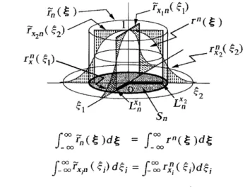
(4) 94. Memoirs of The School of B. O. S. T. of Kinki University No. 11. (2002). The first- and second NDFs are also expressed by. k , (X) k2 (X) k, (Xi). k2 (Xi) =. (1: (1: (1: (1:. BX(p)p(p)dp). (9). -1. B X (p )p(p')p(p - p') dPd P') -1 BX,(Pi)P(P,i)dP,i) -1 Bx, (p,i)p(P,;)P(P,i - p,;)dp,idP,:. r'. = P(J.L)j O'~ is the unit-volume power spectrum, J.L' = (/-L~, /-L;)t, P(/-Li) = p(J.L) BX(J.L) = BXl (/-LdBx 2(/-L2) and BXi (/-Li) = sin2 7r/-Li X ij (7r/-Li X i)2.. where p(J.L). (10) (11) (12) l/-lj=o,(i#j) '. A clear definite relationship between the two-dimensional NDFs kn(X) and the one-dimensional NDFs kn(Xi ) cannot be easily seen. However, if the correlation function r(~) is separable as r(~) = r Xl (6)r X2 (6), then the NDFs kn(X) (n = 1,2) are also separable as,. (13) An alternative second-order NDF can be defined as kc(Xl ) = Var[g(x)g(Xl + 6, X2)] /var[R Xl (6)] (0::; 161 < Xl) where RXl (6) is the sample correlation function defined by RXl (6) = (Xl - 6)-1 J~~~~~~lg(Xl' X2)g(Xl +6, X2) dx l (for 6 2:: 0) and RXl (-6) = RXl (6)· For a large Xl, the approximations Var[g(x)g(Xl + 6, X2)] ~ 20'4 (for smallI6/), ~ 0'4 (for large 16/) and Var[RXl (6)] ~ (2jX l ) J~= R;l (~)d~ (for smallI6/), ~ (ljXt) J~= R;l (~)d~ (for large 161) are obtained [3]. Therefore, kc(Xt) and k2(X l ) are asymptotically equal kc(X l ) ~ k2(X l ). Similarly, k c(X 2) ~ k 2(X 2) and kc(X) ~ k 2(X) are obtained. Hence, the second:...order NDF k2(X) is referred to asymptotically as the amount of information about the correlation function as well as the variance. Consider the Karhunen - Loeve expansion of the field g(x) in the finite area V. Introducing Ak (k = 0,1,2"" ), the eigenvalues of the corresponding Fredholm's integral equation, the second-order NDF k2 (X) is simply expressed as. (14) The above expression agrees with the number of degrees of freedom of the X2-distribution or the gamma-distribution by which the probability density of Z2(X) is approximated.. II. CA AND CL. The CAs and CLs of a random field, if limits exist, are defined as follows:. (15) (16) where Sn is the nth-order CA and L~i the nth-order CL in the direction of the xi-axis. CA refers to an equivalent area over which one point in the field has statistically effective influence..

(5) 95 CL refers to an equivalent distance between two adjacent uncorrelated points on a line in the field. The field g(x) is ergodic in the nth moment if the limit on the right side of (15) exists. When the limit on the right side of (16) exists, anyone-dimensional field on a line parallel to the xi-axis is ergodic in the nth moment. The CAs and CLs for n = 1, 2 can be expressed simply as. I:. (1/2). rn(e)de,. I:. n. = 1,2. r~, (t;i)dt;i,. (17). n = 1,2.. (18). Equations (17) and (18) are obtained by dominated convergence. The terms "CA" and "CL". Figure 1: nth-order CA and CLs in correlation domain, where n. =. 1,2.. come from the expressions (17) and (18). If a correlation function rn(e) (n = 1,2) with a fiat upper surface that is equivalent to r(e) such that rn(O) = r(O) = 1 and J~oo rn(e)de = J~oo rn(e)de is considered, Sn equals the dimensions of the support of rn(e). Thus, Sn becomes a measure that gauges the dimensions of an effective support of the correlation function r(e). However, CAs Sn do not necessarily denote the concentration of the correlation function about the origin. Length 2L~: is equal to the width of the boxcar correlation function rXin(~i) which is equivalent to r Xi (~i) such that rXin(O) = r Xi (0) = 1 and J~oo rXin(~i)d~i = J~oo r;);i (~i)d~i (n = 1,2). These are illustrated in Figure 1. If the correlation function r(e) is separable, we obtain the following simple relationship between CA and CLs:. (19) In the frequency domain, the following expressions are obtained. I:. 8 1 = p(O),. 82. =. p2(J.')dJ.',. Lfi. =. I:. (1/2)P x i (0). L~' = (1/2). p~,(,"i)d,"i. (20) (21).

(6) 96. Memoirs of The School of B. O. S. T. of Kinki University No. 11. (2002). where 0 = (0, O)t and PXi (/-Ld is the marginal spectrum. (22) The equation of the first-order CL Lfi = (1/2) f~ r Xi (~i)d~i in (18) is the same as the definition of Taylor's length (1) or Vanmarcke's "scale of fluctuation" [25], and the first-order CA 8 1 in (17) is the same as Vanmarcke's "characteristic area" [25]. These features playa significant role both in several branches of· physics and in texture analysis. However, there are drawbacks associated with both features. Consider, for example, a damped oscillatory correlation function. The first-order CL and CA may then become extraordinarily small despite the persistence of the correlation function for a finite or infinite range. This effect is counterintuitive. However, because correlation functions in physical diffusion fields or in turbulent flow fields in which Taylor's length has been successfully applied rarely take on a negative value, this factor is not generally a consideration. On the other hand, texture images can possess every possible type of correlation function. As a result, this drawback may strongly influence image processing. Accordingly, the first-order CA and CL may not always be a suitable feature of a texture. Stratonovich's CL [22] in the theory of random processes defined by TS trat = foCX) Ir(~)ld~ provides one means of overcoming this problem. However, their CL does not appear to have any solid theoretical basis or physical relevance. Alternatively, the second-order CA and CL can provide a better alternative to overcome this problem because they are based on statistical theory and are mathematically simpler.. III. EBA AND EBW. We refer to the nth-order NDF per unit area and the nth-order NDF per unit length as the nth-order EBA and the nth-order EBW, respectively. The nth-order EBA On and EBWs W~i can then be defined as lim. X 1 ,X2 ---+CX). kn(X) / Av = 8;;1. lim kn(Xi ) /X i = (2L~i)-1 .. (23) (24). xi---+CX). If the correlation function r(e) is separable, we obtain the following relationship for n = 1,2. (25). A. First-Order EBA and EBW. The first-order EBA and EBWs are expressed as. Wfi = (1/2)p~"/(0).. (26). Consider a two-dimensional spectral density PI (J.L) with a flat upper surface that is equivalent to p(J.L) in the sense that Pl(J.L) = p(O) (J.L E B1 ), = 0 (J.L tf. B1 ) and f~CX)Pl(J.L)dJ.L = f~CX)p(J.L)dJ.L = 1, where Bl is the finite support of PI (J.L). The area of support Bl then becomes equal to the first-order EBA 0 1 . Wfi is referred to as the bandwidth of the bandlimited white spectral density PXi 1 (/-Li) which is equivalent to PXi(/-Li) such that PXi 1 (/-Li) = PXi(O) (I/-Lil ::; Wfi), = 0 (I/-Lil > Wfi) and.

(7) 97. J~oo Pxd (fJ,i)dfJ,i = J~oo PXi (fJ,i)dfJ,i = 1. Note that 0 1 diverges when p(O) ---t 0 and Wfi does when PXi (0) ---t O. Therefore, the first-order EBA and/or EBWs are not applicable to fields with extremely small dc components. Lampard [12] defined the "equivalent duration" 1':1t (= Lfi) and "equivalent bandwidth" 1':1j (= 4Wli) and obtained the identity 1':1t1':1j = 1, which is a special case of n = 1 in (24).. B. Second-Order EBA and EBW. The second-order EBA and EBWs are expressed by. (1: (2. p2(p)dp). 1:p~.. (27). -1 1. (28). (fli )dflr. EBA is referred to as a measure that gauges the area of an equivalent support of the spectrum p(/-L) in the following sense: Consider a spectral density P2 (/-L) equivalent to p(/-L) such that P2(/-L) = const. (/-L E 8 2 ), = 0 (/-L rt. 8 2 ), J~ooP2(/-L)d/-L = J~oop(/-L)d/-L = 1 and J~oo P~ (/-L )d/-L = J~oo p2 (/-L )d/-L, where 8 2 is the finite support of P2 (/-L) . The area of support of P2(/-L), which is the area of 8 2 , then becomes equal to the second-order EBA O 2 . W;i is referred to as the bandwidth of the bandlimited white spectral density PXi 2(fJ,i) which satisfies PXi 2(f.-l) = const. (lfJ,il ::; W;i), = 0 (If.-lil > W;i), J~ooPXi2(fJ,i)dfJ,i = J~ PXi (fJ,i)dfJ,i = 1 and J~oo P;i2(f.-li)df.-li = J~oo p;JfJ,i)df.-li.. PX2 1 (f1- 2) PX22 (. Figure 2: nth-order EBA and EBWs in spectral domain, where n. f1-:0. = 1,2.. In the theory of random processes, the second-order EBW has been used as a measure of the bandwidth of a random process and as an equivalent bandwidth of a window function used in spectral estimation [4]. Furthermore, the EBW is a member of a class of "uncertainty" defined by Zakai [27] and is closely related to the "duration" proposed by Lerner [13]..

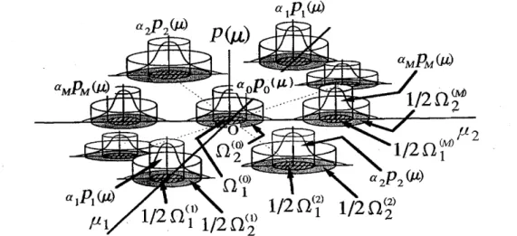
(8) 98. Memoirs of The School of B. O. S. T. of Kinki University No. 11. (2002). Although the first-order EBA and EBWs cannot be effectively applied to fields with extremely small dc components, second-order EBA and EBWs do not possess this problem. When a random field is bandlimited and white as shown in Example1, the first-order features agree with those of the second-order. The first- and second-order EBAs and EBWs are shown in Figure 2.. IV. MULTIMODAL RANDOM FIELD. Let qdp) (k = 0,1"" ,M) be non-negative unimodal functions that satisfy maxp qk(P) = qk(O), qk( -p) = qk(p), and J~oo qk(p)dp = 1. Consider the elementary random field gk(~) which has unit-volume spectra Pk(p) defined by Pk(p) = (1/2) {qk(P - Ck) + qk(P + Ck)}, where Ck = (Ck1' Ck2)t and Ckl, Ck2 = 0 (k = 0), > 0 (k # 0). The Oth elementary field go(~) has a low-pass type power spectrum and gk(~) for k # 0 has band-pass type power spectrum if Ck1, Ck2 (k # 0) are sufficiently large. Assuming that any two supports of spectra Pk 1 (p) and Pk 2 (p) (k1 # k 2) are mutually exclusive, a multimodal random field can be modeled by g(~) = ~~o gk(~)' The unit-volume spectrum p(p) of the multimodal field g(~) is then . M M expressed as p(p) = ~k=O CXkPk(p) , where CXk = Var[gk(~)l/Var[g(~)] ~ 0 and ~k=O CXk = 1. Figure 3 shows an example of the multimodal spectrum.. Figure 3: Multimodal spectrum and spectral features. p(p) = ~~o CXkPk(P) , Pk(P) = {qk(p - Ck) + qk(p + Ck)} , ~~o CXk = 1. In general, n 1 = n~O) / CXo = ~~o (3kn~k). !. ((3k = (CXk/CXO)(qk(O)/PO(O))) and n 2 = 1 /~~o cx~/n~k) . fh diverges when CXo approaches O. If qk(p) are Gaussian, we obtain n 2 =. (~~o(3kn~k))2 /~~o(3~n~k). (30 = (31 = ... = (3M, we obtain n 2 = ~~o n~k).. . Furthermore, if.

(9) 99. A. First- Order Features. Let the first-order quantities Olk) and 8i k) of qk(e) be Olk) = qk1(O) and 8i k) = 1/0lk). Olk) refers to a measure that gauges the band area of Pk (/-L) as shown in Figure 3. Then, if ao -I=- 0, the first-order EBA 0 1 and the first-order SA 8 1 of the multimodal field g(e) are obtained as 0 1 = OlO) lao and 8 1 = a 0 8iO), respectively. The features depend only on ao and the first-order quantities of the Oth elementary field. However, because parameter ao contains information of the other elementary fields if ao -I=- 0, the following expressions including the first-order quantities of the other elementary fields can be expressed by. (29) k=O. (30) where 13k = (akqk(O)) /(aopo(O)) is the ratio of the maximum of the kth spectrum to that of the Oth spectrum. In general, the following inequalities hold:. If 130. = 131 = .... ~. L:~o ( Olk)) 2 ~ L:~o Olk). (31). L:~o (1/8ik))2 ~ 1/L:~0(1/8ik)).. (32). 13M = 1 holds true, then the following simplified expressions are obtained: (33). k=O 81. =. k 1/ L:~0(1/ 8i )) ~ (M. + 1)-2 L:~o 8ik).. (34). In addition , if 0(0) = 0(1) = ... = O(M) 0 1 = (M + 1)0(0) and 8 1 = _1_8(0) 1 1 1 , 1 M+1 1 are obtained . The first-order features 0 1 and 8 1 are not applicable to the multimodal field when the power ao of the Oth elementary field go(e) is extremely small.. B. Second- Order Features. Let O~k) and 8~k) denote the second-order quantities of the unimodal function qk(e) as O~k) = 1/ J~oo q~(/-L )d/-L and 8~k) = 1/0~k). Then, the second-order features O 2 and 8 2 of the multimodal random field g(e) can be expressed as. (35) M. 82. =. La~8~k). k=O. (36). O~k) is an alternative measure of the band area of the kth spectral component Pk(/-L) as shown in Figure 3..

(10) 100. Memoirs of The School of B. O. S. T. of Kinki University No. 11. (2002). In general, the following simplified inequalities hold true:. 2:!o (1/0~k)) 2:!o (8~k)) If ao. = al = ... =. 2. 2. 2. (2:!o 1/0~k))-1. (37). ~ 2:!o 8~k). (38). aM, then. (39). (40) In addition, if O~o). V. = 0~1) = ... = O~M), then. O2. = (M + l)O~O) and. 82. = 8~O) /(M + 1).. EXAMPLES. In order to study how the present features characterize a random field and how they are interrelated, we examine several examples of typical random fields.. Example 1 (BandLimited White Field) Let us consider a bandlimited white field which has the unit-volume power spectrum. l/-Lll ~ W X1 and 1/-L21 ~ W X2 otherwise.. (41). As the correlation function r(e) becomes separable, the NDFs in the rectangular area V, the CAs, and the EBAs for n = 1,2 become separable as in (13), (19) and (25). The first- and second-order EBWs are obtained as Wfi = W:fi = W Xi and the EBAs as 0 1 = O 2 = 4WX1 W X2 ' The CLs and CAs can then be expressed as Lfi = L~i = (4WxJ- 1 and 8 1 = 8 2 = (4WXl W x2 )-I. For a sufficiently large Xi, NDFs are approximated by kn(X) ~ (2WX1Xl)(2WX2X2), kn(Xi ) ~ 2Wxi X i for both n = 1 and n = 2. Any two of the random variables sampled at the Nyquist rate of 2WXi on a line parallel to the xi-axis are not correlated with each other. Therefore, the average number of uncorrelated variables in the interval Xi should be 2WXi Xi and the number of uncorrelated variables in the area V should be (2WXl X 1 )(2Wx2 X 2), The above results conform to these rules.. Example 2 (Field of Plane Waves) Consider a field defined by a linear combination of a finite number of plane waves. Suppose the field g( x) is given by K. g(x). L{. am. cos 27r J1,~ X. + bm sin 27r J1,~ x },. (42). m=1. where am, bm are independent Gaussian random variables with zero mean and variance Var[a m ] = Var[b m ] = ()~ and J1,m = (/-LIm, /-L2m)t is the spatial frequency vector. If the spatial frequency.

(11) 101 /-Lim satisfies the conditions /-Lim > 0 and /-Lim function r(~) can be obtained as follows:. =1=. n), the normalized correlation. r(~) = ~ L O"~ cos 21fJ-t~x,. (43). /-Lin (m. =1=. K. O"g. m=l. 0";. where = L~=l O"~. Although the oscillatory correlation function r(~) is not absolutely integrable, we can calculate kn(X) and kn(Xi ) and study their asymptotic behavior for Xl, X 2 ---+ 00.. In this sense, the first-order NDFs are kl (X) = 1 /. O(X?X~), kl(Xi ) =. 1/ ;~ L~=l O"~BXi(/-Lim). ;~ L~=l O"~BXI (/-Llm)B x2 (/-L2m). =. O(Xf). Thus, kl(X)/A v , kl(Xi)/Xi ---+ 00 when Xl and/or X 2 ---+ 00. In other words, the unit area and unit length of this kind of field have infinite information about the first moment. Consider, for example, an inversely correlated random sequence {ud (COV[Ui,Ui+l] /Var[ui] = -1). In such a case, two consecutive samples may be sufficient to accurately estimate the mean value of {Ui}. Thus, the two samples would possess infinite information about the mean. Strictly speaking, since the variance of the sample =. M. mean U = (1/ M) LUi is proportional to M- 2 , kl (M). = O(M2) and kl (M) / M. ---+ 00. (M---+. i=l. (0) are obtained. In addition 8 1, Lfi. ---+. 0 and. nl , Wfi. ---+ 00. when Xl and/or X 2 ---+. Next, the second-order NDFs are k 2(X) = 20": /L~=l. . BXI (/-L2m (m. + /-L2n) + BXI (/-LIm -. = n), = O(X12 X22) (m. {I + O(Xi- 2)} (m. =. n),. lim. X I ,X2 --+00. =. 00.. L~=l O"~O"~ {Bx I (/-LIm + /-LIn). /-Lln)B XI (/-L2m - /-L2n)} = (20": /L~=l. O"~ ) {I + O(X12 X22)} k 2(X i ) = (20": /L~=l O"~). n). Similarly, O(Xi- 2) (m =1= n) are obtained, resulting in: =1=. k2(X). =. lim k 2(X i ) = Xi--+OO. 2(L~=1 0"~)2/ L~=l O"~.. (44). The right side of the above equation is similar to the expression in (14). If O"r = O"~ = ... = O"k' we obtain limx l ,x2 --+oo k 2 (X) = limxi--+oo k 2 (X i ) = 2K; namely, for sufficiently large Xl, X 2 the second-order NDFs become equal to the number of the independent coefficients am, b m . This is intuitively sound. 8 2, L~i ---+ 00 and n2 , W;i ---+ 0 are obtained when Xl and/or X 2 ---+ 00 because the field has a periodical correlation function and a line spectrum.. Example 3 (Field with a Gaussian Correlation Function) Consider a field with a Gaussian correlation function. (45) where A = (aij) is a symmetrical positive definite 2 x 2 matrix in which aii > O. Let Ai > o (i = 1,2) be the eigenvalues of A. Then, the first- and second-order CAs Sn are expressed as:. Sn = (21f/n)/yiAlA2,. n = 1,2.. (46). The CAs are equal to the dimensions of the elliptic cross section represented by ~t A~ = 2/n of the correlation function rn(~) at a height of e- l ...

(12) 102. Memoirs of The School of B. O. S. T. of Kinki University No. 11. (2002). The first- and second-order CLs are. L~i = (1/2)j(27r/n)/aii'. n = 1,2.. (47). L~i is equal to half the distance between two points on the ~i-axis at which the correlation function r~i (~i) is equal to e-11'/4. In other words, L~i is half the distance between the two = 7r/(2n). The EBAs and EBWs are easily intersections of the ~i-axis and the ellipse obtained from (23) and (24). Since A is symmetrical, the inequality AIA2 ::; alla22 holds true. Hence, from (46) and (47) the following inequalities are obtained:. etAe. n. = 1,2,. (48). where the signs of equality hold true if and only if A is a diagonal matrix; that is, the correlation function is separable. When we rotate the 6 -6 plane so that A becomes diagonal, the directions and quantity of the CLs agree with those of the principal axes of the ellipse = 7r/(2n). Then, denoting the lengths of the principal axes by L~ajor and L~inor, the following relationship is always obtained:. etAe. 4L nmajor L nminor ,. (49). n = 1,2.. Similarly, we obtain 4wnmajorwminor n ,. w:. n. 1 2. (50). =". w:. ajor inor where and denote EBWs in the direction of the principal axes. The principal axes problem is discussed in more detail in Section VI. Furthermore, we find the following relationships between the first- and the second-order features:. Lfi. 8 1 = 282 ,. 01. =. = V2L~i. (51). Wfi = (l/V2)W;i.. (1/2)0 2 ,. (52). Example 4 (Multimodal Field Composed of Gaussian Spectral Components) Consider the Gaussian functions k = 0,1"" ,M,. (53). where Ak = (a~j) are symmetrical positive definite 2 x 2 matrices in which a~;) > O. Then, as introduced in Section IV, we consider a multimodal random field composed of M elementary random fields which has unit-volume power spectra defined by Pk(/-L) = (1/2) {qk(/-L - Ck) + qk(/-L + Ck)} Application of the results in Example 3 yields the nth-order quantities of the kth elementary field as S~k) = l/n~k) = (21r/n) / Aik) A~k) for n = 1,2, where A)k) denote the eigenvalues of. A k . The relationship 20~k) = O~k) holds true. Then we obtain. -1 L{3k M. 27r. A(0) A(0) 1. (54). 2. k=O. (I:~o fA. 1 A(k) A(k). 1. 2. ,\",M 7r Dk=O. Aik). (32 k. A~k)) 2 (55). dk-) dk). /\1. /\2.

(13) 103 We also find the expression O = ,8kO~k)) ,8~O~k). If all the relative magnitudes of the component spectra are equal, that is, if ,80 = ,81 = ... = ,8m, then the following simplified expressions are obtained:. 2 (2::"0. 2/ 2::"0. M. On. = LO~k),. n = 1,2.. (56). k=O. =. (~. i. ) , B2 - A,A2 < 2 0, Al > 0, A2 > O. Consider a random field g(x) described by an elliptic partial differential equation (PDE). Exrunple 5 (Field Described by an Elliptic PDE) Put P. (57) where li. = (a/Xl, a/X2, I)', Pe =. (~ ~I). and €(x) is a two-dimensional white noise. process. Expression (57) is often used as a noncausal model for texture images [7]. The normalized correlation function r(~) and unit-volume power spectrum p(J-t) of g(x) are then given by. Vep-'f.K, (Vf.'P-If.). and. 4'wVdet P / (47r 2J-tt P J-t + 1)2,. p(J-t). (58) (59). where K 1 ( .) is the modified Bessel function of the second kind of order l. If the eigenvalues of P are represented by Pk > 0 (k = 1,2), the CAs and CLs are obtained as. (1/3)n- 1 47rVPIP2,. (3/8) n-l( 7r /2)n The following relationship between Sn and. JPIP2/A. L~i. (60). n = 1,2, j ,. i. -I j,. n. = 1,2.. (61). always holds:. n. = 1,2.. (62). The equality in the above expression holds if and only if P is a diagonal matrix. The last inequality in (62) states that the correlation function of any random field described by an elliptic PDE cannot be separable. The relationships SI = 3S2 and Lfi = (16/37r )L~i also hold. The EBAs, EBWs, and their relationships are easily obtained from the above results.. Example 6 (Field Described by a Hyperbolic PDE) Let P be negative definite; that is, B2 - AIA2 > o. The hyperbolic class of PDEs can then be described by (63) where Ph = ( : '. ~I)'. d. (Dl' D 2)t, and D 1 , D2 are real numbers. If the following. condition holds:. (64).

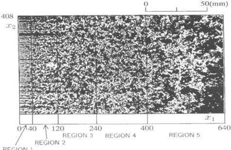
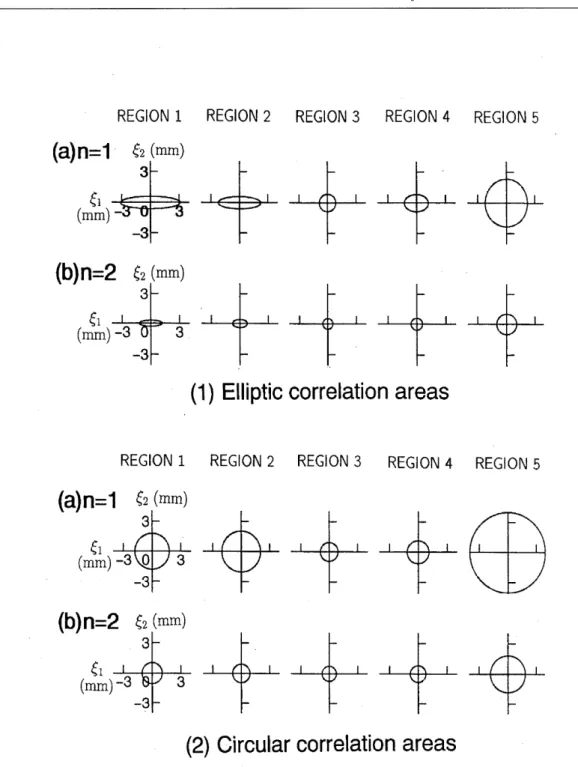
(14) 104. Memoirs of The School of B. O. S. T. of Kinki University No. 11. (2002). then r(e) and p(J.L) are obtained as (65) where. Q. 1 I det PI. (-A2. B--JIdetPT 2. 8vl det PI / Since det P = follows:. AlA2 -. B2 = PlP2. B+JI det PI). ( (47r J.Lt P J.L. «. (66). -AI. + 1) 2 + 167r 2J.Ltdd t J.L). .. (67). 0), the CAs and CLs for n = 1,2 are obtained as. 1,2. (68). n = 1,2.. (69). n i =1= j,. The following relationship between Sn and. L~i. =. for n = 1,2 always holds:. n = 1,2.. (70). Sl = 4S2 and Lfi = 2L~i are also obtained. Whenever the condition (64) is satisfied, the correlation function always becomes separable by rotating the plane Xl-X2 using an orthogonal transformation. For the sake of simplicity, _.l.lhl_.l~. O. Then r(e) = e 21 D II 21D21 = r XI (6)r X2 (6) can be obtained, resulting in L~i = (2/n)IDil, Sn = (4/n)2ID l IID 21, and Sn = 4L~IL~2. The EBAs, EBWs, and their relationships are omitted here.. put. Al = A2 =. Example 7 (A Simple Example of Image Processing) Figure 4, which was presented by Corke and Nagib in [24], shows a turbulent field behind a fine grid which was visualized by the smoke wire method. A uniform laminar stream passes through a plate with square perforations smaller than 3/4-inch. The Reynolds number is 1500 based on the I-inch mesh size. From the figure, we can see qualitatively that the merging unstable wakes behind the grid quickly form a homogeneous and isotropic turbulent field downstream. The figure was sampled into binary form at 100 dots per inch using an image scanner that was connected to a digital computer. The binary field was divided into 5 strips called Region 1, Region 2, ... , Region 5 in ascending order of width. Each region was assumed to be internally homogeneous. The Xl-axis was set parallel to the flow direction and the x2-axis perpendicular. The CAs and CLs were calculated lising the correlation function estimated by r(e) = sin ((7r/2)rs(e)) [15], where rs(e) is the sample correlation function of the sampled binary data. In Figure 5, changes in the CLs and CAs with the location in the flow direction are visualized by drawing equivalent ellipses and circles. Figure 5(1) shows the equivalent ellipses for which the lengths of the two principal axes are equal to (2/ y7i)L~l and (2/ y7i)L~2, respectively, where the directions of the principal axes are assumed to agree with the coordinate axes. In Regions 1 and 2 near the grid, L~l is larger than L~2. In Region 3, however, L~l becomes considerably smaller and reaches a minimum, whereas L~2 increases to almost the same level as L~l. Subsequently.

(15) 105. 50(mm) I. 408 X2. 240 REGION 3 REG ION 2. 400 REGION 4. REG I O N 5. REGION 1. Figure 4: TUrbulent field visualized by smoke wire method. Photograph by Thomas Corke and Hassan Nagib. both. 1-~ 1. and 1-:;2 increase from Regions 4 to 5. Figure 5(2) illustrates the equivalent circles. J. such that the radius of each circle equals the correlation radius dC'fined by RII ~ 8 11 /n . From the figure. we can see that the CAs decrease gradually at first. reach a minimum around Region 3 or 4, and then increase from Regions 4 to 5. These quantitative results support the qualitative characteristics of the flow and conform with current understandings of fluid mechanics.. VI. PROBLEM OF PRINCIPAL AXES OF CORRELATION LENGTH. The CLs depend on the Cartesian coordinate system which can be chosen arbitrarily. However, if the contours of the correlation function r(e) or the power spectrum p( p,) are specified by a symmetric matrix such as A in Example 3 or P in Example 5 and Example 6. we can find the major and minor principal axes and corresponding CLs that are inherent in the field. In this section, we consider the principal axes problem for a field with the Gaussian correlation function shown in Example 3. The symmetrical matrix A in (45) is transformed into a diagonal matrix AI by an orthogonal transformation with an orthonormal matrix U. Denote the principal axes system by x~ -x~. If () denotes the angle between systems XI-X2 and x~ -x~. the orthonormal matrix U and the diagonal matrix AI are given by U = ( c~s ()() - sin()() ) and AI = U t AU = (Ai6i)'), where 6i]' , sm cos ' is Kronecker delta. The correlation fUllction rl ((). where ( = ((~, (~) f • in Cartesian coordinate. e.. system x~-x~ is written as rl (() = e-~e' AI Redefine the smaller eigenvalue A'i as A1l1ajor and the larger as Aminor. If au in (47) is replaced by All1ajol or Alllillor, the major and minor CLs for rz = L 2 are obtained as L~~lajor = (1/2) (nA ll1 a j or) and L:~1il1or = (1/ (2) (nAlI1 inor) .. J2n /. J2n /.

(16) 106. Memoirs of The School of B. O. S. T. of Kinki University No. 11. REGION 1. REGION 2. REGION 3. REGION 4. (2002). REGION 5. (a)~:++++~ (b)(~~f +. + ++. (1) Elliptic correlation areas REGION 1. REGION 2. REGION 3. REGION 4. REGION 5. (a:~:~ +. + + EB. (b)(~:+ +. +++. (2) Circular correlation areas Figure 5: Changes in CAs for n = 1,2. (1) Equivalent ellipses; major and minor axes of each ellipse are (2/ ft)L~l and (2/ ft)L~2, respectively. (2) Equivalent circles; each circle has radius. Rn. =. y' S n/ 7r •.

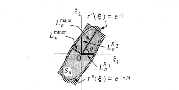
(17) 107. e -1. L~l. ~1. r n( ~ ) = e - IT /4 Figure 6: CAs and CLs for a Gaussian correlation function. nth-order CA equals area of ellipse rn(~) = e- 1 and agrees with area of rectangle 2L~ajor x 2L~inor, where n = 1,2.. Although matrix A is rarely known in advance in practical applications, it can be obtained from A =. (l/n)~~l (n = 1,2), where ~n = ((]":l) and (]":l = J~oo ~i~jrn(~)d~ / J~oo rn(~)d~ =. (]"~i. Accordingly, we can calculate the eigenvalues and then the principal CLs.. Since the correlation function rl(~/) is separable, the equation Sn = 4L~ajor L~inor (n = 1,2) holds. The nth-order CA, the nth-order CLs and their interrelationships are shown in Figure 6. Sn (n = 1,2) equals the area of the ellipse expressed by the equation rn(~) = e- 1 as well as the area of the rectangle 2L~ajor x 2L~inor. CL L~ajor and CL L~inor for n = 1,2 can be obtained by Sn and L~i without calculating matrix A. The two eigenvalues A's satisfy the characteristic equation IA - .\EI = 0, where E is the unit matrix. Furthermore, Sn is expressed as Sn = 27T"/ (n det A) and L~i is given by (47). Hence, the eigenvalues can be expressed as (71) where l~ = 2(L~1 L~2)2 /((L~1)2 + (L~2?). Consequently, if (71) is substituted into L~ajor = (1/2) V27T"/(n.\major) and L~inor = (1/2) V27T"/(n.\minor), we obtain the major CLs and minor CLs as. L::>ajoc. L;:,inoc. =. In /. Vl-. )1- (4l'!,/Sn)2 ,. n. = 1,2. (72). In /. Vi +. )1-. (4/~/Sn)2 ,. n. = 1,2. (73). Angle B satisfies tan2B = 2a12/(all - a22). Therefore,. B = (1/2)'Po,. -7r. /2 < 'Po < 7r /2,. (74).

(18) 108. Memoirs of The School of B. O. S. T. of Kinki University No. 11. (2002). where <Po is the principal value of <p = tan -1 2a12/ (all - a22). If all < a22, i.e. L~l > L~2, e represents the angle between the major CL and xl-axis. The angle becomes positive for a12 < 0 and negative for a12 > O. In contrast, if all > a22, i.e. L~l < L~2, e represents the angle between the minor CL and xl-axis where the angle is negative for a12 < 0 and positive for a12 > o. If all = a22 and a12 < 0, the angle between the major CL and xl-axis equals 7T / 4 and the angle between the minor CL and xl-axis is -7T / 4. Conversely, if all = a22 and a12 > 0, the former is -7T / 4 and the latter equals 7T / 4. In order to express the angle e in terms of Sn and L~i, we have to represent all, a22 and a12 using Sn and L~i. The components aii and a12 can be expressed as aii = (7r /2n) (L ~i) -2 and a12 = ±(7T/2n)(L~lL~2)-lJ1- (4L~lL~2/Sn)2, respectively. However, the sign of a12 cannot be decided on the basis of Sn and L~i alone. One method for determining the sign is to use the quantity CJ;( = -a12/(alla22 - a12a21). Since the relationship sgn(a12) = -sgn(CJ~2) always hold true, angle e can be obtained from the following equation:. VII. CONCLUSION. We have extended the idea of nth-order NDF of a one-dimensional random process to a twodimensional Gaussian random field and the nth-order (mainly n = 1,2) features CAs, CLs, EBAs, and EBWs have been deduced from the NDFs. The class of the first-order features contains the well-known Taylor's CL (or Vanmarcke's scale of fluctuation) and Vanmarcke's characteristic area. The properties of the features of a field with multimodal spectrum have been examined in detail. Several examples of different typical random fields and a simple example of image processing have been presented in order to understand the properties of the features and their role in image processing. Although the first-order features are simple basic measures that characterize random fields and have been demonstrated to play an important role in many physical fields, they are not applicable to fields with extremely small dc components, such as band-pass type fields. In contrast, second-order features, which are also simple, are effective for a large class of random fields that contains both low-pass type and band-pass type fields. We have discussed the problem of principal axes in relation to the CLs of a field with a Gaussian correlation function. The principal CLs have been expressed in terms of CAs and CLs on an arbitrary Cartesian coordinate system. The expressions may provide a practical method of calculating the principal CLs when the matrix that characterizes the correlation function is not known.. Acknowledgement: This study was supported in part by the Ministry of Education of Japan Grants in Aid for Scientific Research (No. 06301031 and No.08680336) and the Grants in Aid of Kinki University (No.GG44 and No.9666).. References [1] Yu. D. Arbuzov, V. M. Evdokimov, and M. Yu. Lolenkin. Interband light absorption in heavily doped semiconductors in the deep tail region. Cov. Phys. JETP , 65(4):758-761, 1987. [2] R. Bajcsy. Computer description of textured surfaces. In Proc. 3rd Int. ConE. on Artifical Intelligence, pages 572-579, 1973..

(19) 109. [3] J. S. Bendat and A. G. Piersol. Measurement and analysis of random data. John Wiley & Sons, Inc, 1958. [4J R. B. Blackman and J. W. Tukey. The measurement of power spectra from the point of view of communications engineering--Part I, II. Bell Syst. Tech. J. , 37(1):185~282, 485-569, 1958. [5J F.R.S. G. 1938.. r. Taylor.. The spectrum of turbulence. Proc. Roy. Soc., London, AI64:476-490,. [6J J. O. Hinze. Turbulence. McGraw-Hill, Inc., 1975. [7J A. K. Jain. Partial differential equations and finite differences in image processing, Part I-Image representation. J. Optimiz. Theory and Appl., 23:65-91, Sept. 1977. [8J F. C. Jones and T. J. Birmingham. Investigation of resonance integrals occurring in cosmicray diffusion theory. The Astrophysical Journal, 181:L139-L142, 1973. [9J H. Kaizer. A quantification of textures on aerialphotographs. Tech. Note 121, AD 69484, Boston University Research Laboratories, Boston University, 1955. [10J S. Kikkawa. Number of degrees of freedom, Fisher's informations, and frequency-time products of a random process. Electronics and Communications in Japan, Part 3:Fundamental Electronic Science, 77(3) :28-39, 1994. [llJ S. Kikkawa and M. Ishida. Number of degrees of freedom, correlation times, and equivalent bandwidths of a random process. IEEE Trans. Inform. Theory, 34(1):151-155, 1988. [12J D. G. Lampard. Definition of 'bandwidth' and 'time duration' of signals which are connected by identity. IRE Trans. Circuit Theory, CT-3:286-288, 1956. [13J Lerner. R. M. Means for counting 'effective' numbers of objects or durations of signals. In Proc. Inst. Radio Rngys, volume 47, page 1653, 1959. [14J A. S. Monin and A. M. Yaglom. Statisticheskaya gidromekhanika" volume I, II. Moskwa, 1967. Statistical fluid mechanics, Vols 1 and 2, MIT Press, Cambridge, 1971, 1975. [15] A. Papoulis. Probability, random variables and stochastic processes. McGraw-Hill, Inc., 1965. [16J Fai Ma Peter Bouton. On spatial dependence in monte carlo simulations of random fields. International Journal of Modeling and Simulation, 8(3):94-97, 1988. [17] B. Porat and B. Friedlander. On the estimation of variance for autoregressive and moving average processes. IEEE Trans. Information Theory, IT-32(1):120-125, 1986. [18] S. O. Rice. Mathematical analysis of random noise, Part III. Bell Syst. Tech. J. , 24:46-165, 1945. [19] A Rosenfeld. Visual texture analysis: An overview. Computer Science Technical Report, TR-406, F44620-72C-0062:1-11, 1975. University of Maryland. [20] C. C. Shih. Quantum-statistical analysis of charge correlations in multiparticle production at high energies. Physics Letters B, 259(4):293-298, 1991. [21] D. Slepian. Fluctuations of random noise power. Bell Syst. Tech.J. ,37:163-184, 1958..

(20) no. Memoirs of The School of B. O. S. T. of Kinki University No.ll. (2002). [22J R. L. Stratonovich. Topics in the theory of random noise, volume 1. Gordon and Breach, New York, 1963. [23] G. 1. Taylor. Diffusion by continuous movements. Proc. London Math. Soc. (2),20:196-211, 1921. [24] Milton Van Dyke. An album of fluid motion. The Parabolic Press, Stanford,. California, 1982. [25] E. Vanmarcke. Random fields, analysis and synthesis. The MIT Press, 1983. [26J J. S. Weszka, C.R. Dyer, and A. Rosenfeld. A comparative study of texture measures for terrain classification. IEEE Trans. Syst. Man. Cybern., SMC-6(4):269-285, 1976. [27] M. Zakai. A class of definitions of 'duration' (or 'uncertanty') and associated uncertainty relations. Inform. Contr., 3:101-115, 1960.. $~G~<::J:Jl~~<::!E~~tLTv\~. 1 ~nlit*~;fjO)~fE~tB~§EI3J3tO)m~~fflv\, 2 ~. nut*t~0)~fE~tB~4~f~t~0)~m~J:\~¥Jte ~§OO~~. tf§OOOO;fJL MtH<::,. GtL.O. .:c0)4~flm t ~i, lit*t~O)~ 1JrtiH<::xt9 ~. 2 ~nmJrBl~)(~Ji~~<:::f3~t~~{[ffim~~Mt~{[ffi*~rnImC'd0. v\ <JiJ\0){-\:;*B~ut*t~0)1JU~<::Xt9 ~ <:nG!WtflmO)J!I;K~vvI1~ 'baA GiJ)~<:: G tL.O ~ G~;:, @j{~9J1f!A,.O)Jitffl 0)1JU t G l, *~ §~~r1~mt~;: tHt ~ ~Lmt@j{~O)M~fJT~~i\djtL.O ~ G~;:, lit*t~O)f§I~~H<::OO9 ~±'mri:mmt~§OO~~ t O)OO{*~;:JV\l 'bJm«tL.O *WB)(C' ~o. ¥J~tLk~M~!Wtfla~lit*~t.:c0)~~~~~~~~Jm9~~~~.1;K0)~lit~'b0)C' d0~,@j.MfiA,.O)Jitffl~M~~h~o~~m~,$~~&[email protected][email protected],. 0) Jitffl ~ ~i\dj J. J. d0 ~. 0.

(21)