A Study on Fermionic Wiener
Functionals via Stochastic Areas and
its Applications
Hidemi Aihara
Ritsumeikan University
Contents
1 Tau functions of KP solitons realized in Wiener space 5
1.1 Introduction . . . 5
1.1.1 Solitons, tau-functions, and Sato’s Grassmannian . . . 5
1.1.2 Probabilistic approach to solitons . . . 8
1.1.3 Organization of the present paper . . . 9
1.2 A generalization of L´evy’s stochastic area formula . . . 9
1.3 Parameterization as a tau function of KP solitons . . . 12
1.4 Reduction to Ikeda-Taniguchi’s construction . . . 14
2 Affine term structure as multi-soliton 16 2.1 Introduction . . . 16
2.2 A primitive example . . . 18
2.2.1 Solitons . . . 19
2.3 Affine Term Structure as Multi-Soliton . . . 20
2.4 Remarks on a relation with KdV equation . . . 24
2.5 Parameterization as a tau function of KP solitons . . . 24
2.6 Reduction to Ikeda-Taniguchi’s construction . . . 25
3 Wiener Functionals as Fermions and their Bosonization via Stochastic Areas 27 3.1 Introduction . . . 27
3.1.1 What is done in this section? . . . 27
3.1.2 Why a probabilistic Bosonization is important? . . . . 28
3.1.3 The Organization of the Present Section . . . 29
3.2 Fermions and Bosons . . . 29
3.2.1 Heisenberg Algebra . . . 29
3.2.2 Clifford Algebra . . . 30
3.2.3 Vacuum Expectation Value . . . 31
3.2.4 Bosonization . . . 31
3.2.5 Young Diagrams . . . 33
3.3 A Probabilistic Bosonization . . . 34
3.3.1 A Realization of Fermions in Wiener Space . . . 34
3.3.2 The Vacuum Expectation in Wiener Space . . . 35
3.3.3 A Bosonization . . . 38 3.3.4 A Probabilistic Bosonization in terms of Stochastic Areas 40
4 Some Universal Properties of Stochastic Areas 43
4.1 Introduction . . . 43
4.2 A Generalization of the L´evy-Area Formula . . . 44
4.3 Proof of Theorem 21 . . . 45
Abstract This thesis is organized into four sections.
In the first section, a probabilistic representation of the tau func-tions of KP (Kadomtsev-Petviashvili) solitons in terms of stochastic areas will be presented.
The second section is composed of a remark that Quadratic Gaus-sian term structures under suitable scale change are of multi-soliton type, (a collection of) solitary waves that are related to KdV solitons. In the real market, the term structure of forward rates exhibits some humps. The quadratic Gaussian term structure models or affine term structure models well explain this phenomena.
The third section presents a probabilistic “Bosonization” using stochastic areas. With the Bosonization, the “Fermions”, which are anti-symmetric stochastic integrals generated by a representation of a Clifford algebra in Wiener space, are sent to the character poly-nomials. This Bosonization enables us to construct a probabilistic representation of tau functions of integrable systems.
In the last section, we present two equivalences in law among stochastic areas. The first one states that the law of a stochastic area at a fix time of a Gaussian process(stochastic integral of a deter-ministic L2 function) is only dependent on its L2-norm. The second one is on the pair of (generalized) stochastic areas. It says that the law of a pair related to Walsh system is again independent of the choice of the Walsh function.
1
Tau functions of KP solitons realized in
Wiener space
1.1
Introduction
In the introduction, after giving a very short introduction to the theory of solitons following [24], we recall some existing results from probabilistic approaches.
1.1.1 Solitons, tau-functions, and Sato’s Grassmannian
By solitons, we usually mean solitary wave solutions (behaving like a particle) to a class of non-linear wave equations including the KdV (Korteweg-de Vries) equation ∂u ∂t = 1 4 ∂3u ∂x3 + 3 2u ∂u ∂x (1.1)
as the most notable example.
The first giant step in the study of solitons was made by Gardner, Greene, Kruskal and Miura [7], where they observed that (i) the eigenvalues of the Shor¨odinger operator
∂2
∂x2 + u(t, x),
where u is a solution to (2.16), are constant in time parameter t, and (ii) one can construct a soliton solution to (2.16) by applying the inverse
scat-tering method, by which we mean the (mathematical) method to construct
(unknown) potentials out of given scattering data, which had already been fully developed. The relation is most clearly seen when the potential is
re-flectionless as u(t, x) = 2 d 2 dx2 log det(I + G(x, t)), (1.2) where G(x, t) := (√m imje(ηi+ηj)x+(η 3 i+ηj3)t ηi+ ηj ) 1≤i,j≤n .
The constants ηj, mj, j = 1,· · · , n are so-called scattering data.
The observation (i) together with the awareness of the existence of the infinite invariants in [7] motivated another seminal paper by P. Lax [20],
where the KdV equation (2.16) is understood as the compatibility between the two equations:
( ∂2 ∂x2 + u(t, x) ) w(=: P w) = κw, (κ is an eigenvalue) ( ∂3 ∂x3 + 3 2u ∂ ∂x+ 3 4 ∂u ∂x ) w(=: Bw) = 0.
This compatibility is rephrased as the celebrated “Lax equation”:
∂P
∂t + [P, B] = 0, (1.3)
where the bracket is the commutator; [P, B] = P B− BP .
By considering pseudo differential operators such as ∂−n for n ∈ N and their infinite series, we have in fact B = (P3/2)+, where (D)+ is the
differ-ential operator part of the pseudo differdiffer-ential operator D. In this Lax form, the existence of the infinite many invariants can be rephrased as
∂P ∂xk
+ [P, (Pk/2)+] = 0, k = 1, 3, 5,· · · , 2n + 1, · · · ,
where u ≡ u(x1, x3,· · · , x2n+1,· · · ), a function of infinitely many variables.
The KdV case (1.3) is retrieved by setting x1 = t, x3 = x. Each Lax
equa-tion generates a non-linear evoluequa-tion equaequa-tion with respect to x2k+1 since
[P, (Pk/2)+]’s are all multiplication operators. The totality of the generated
equations is usually called KdV hierarchy. If we instead start with the operator
L = ∂ +
∞
∑
j=1
uj∂−j,
then we still have that [L, (Lk)
+] are all multiplication operators, and hence
we obtain infinitely many nonlinear differential equations with respect to uj’s
of infinitely many variables x1, x2,· · · , xn,· · · by the Lax equations:
∂L ∂xk
+ [L, (Lk)+] = 0, k = 1, 2,· · · .
The family is called KP hierarchy since the KP (Kadomtsev-Petviashvili) equation, 3 4 ∂2u1 ∂x2 2 = ∂ ∂x1 ( ∂u1 ∂x3 − 3 2u1 ∂u1 ∂x1 − 1 4 ∂3u1 ∂x3 1 ) ,
which is easily seen to be a generalization of the KdV to a two dimensional model, is deduced from the equations with k = 2 and k = 3. The KP hierarchy as a whole is also a generalization of the KdV hierarchy since the latter hierarchy is obtained by a reduction (L2)
− = 0 from the former.
The equations in KP/KdV hierarchy are all “soliton equations” in the sense that they all have exact solutions of soliton type1. In fact, according to Sato’s theory of infinite dimensional Grassmannian ([30], see also [24, 29]), all the uj’s of the hierarchy are simultaneously generated from a single function
called tau-function τ in the following way: determine w1, w2, etc, by
τ (x1−k1, x2− 2k12,· · · ) τ (x1, x2,· · · ) = 1 + w1 k + w2 k2 +· · · (1.4)
by comparing the coefficients of k−j, j = 1, 2,· · · , and then u1, u2, etc by
L = ( 1 + ∞ ∑ j=1 wj∂−j ) ◦ ∂ ◦ ( 1 + ∞ ∑ j=1 wj∂−j )−1 . (1.5)
For example, we have
u1 = 2
∂2 ∂x2
1
log τ. (1.6)
In particular, we see that if τ is a polynomial of e∑cijxj’s, then u
j’s are all
“solitons” in that they are all rational functions of e∑cijxj’s.
The tau functions are characterized as a solution to a family of quadratic differential equations called Hirota equations, which are nothing but Pl¨ucker relations that define Sato’s infinite dimensional Grassmannian. That is to say, a tau function of the KP hierarchy is a point in the Sato’s Grassmannian. It should be noted that in the Sato’s theory, the KP hierarchy is the most universal one, out of which many well-known soliton equations are obtained by a reduction.
The following functions are known to be among the tau functions of the soliton solution of the KP equation:
τ (x1, x2,· · · ) =∑ J⊂I ( ∏ i∈J mi ) ( ∏ i,i0∈J,i<i0 (pi− pi0)(qi− qi0) (pi− qi0)(qi− pi0) ) exp ( ∑ i∈J ∞ ∑ l=1 (pli− qil)xl )
1The solitons are basically rational functions of the exponential functions of the form
e∑cijxj for some constants c
for I ={1, · · · , n}, n ∈ N, where m1,· · · , mn, p1,· · · , pn, and q1,· · · , qn are
(indefinite) constants. This is alternatively written as
τ (x1, x2,· · · ) = det(I + G(x1, x2,· · · )), (1.7) where G(x1, x2,· · · ) = (√m imj pi− qj e12 ∑∞ l=1{(pli−qil)+(plj−qjl)}xl ) 1≤i,j≤n .
The formula (1.7) is a generalization of (1.2) since we retrieve it by (21) and the reductions of qj =−pj, xl= 0 for l ≥ 4.
Remark 1. It should be noted that, if f is a solution to a Hirota equation then
so is Ce∑jcjxjf , for arbitrary constants C, c
1, c2,· · · . Therefore tau function
is stable under the multiplication of the factor Ce∑jcjxj. This property will be used in the proof of Theorem 7.
1.1.2 Probabilistic approach to solitons
As far as we know, the first attempt to represent solitons in terms of the expectation of Wiener functionals was made by S. Kotani [17] in 2000. Ac-cording to [14], Kotani constructed the following correspondences. Let Σ be the set of all pairs (σ+, σ−) ≡ σ of non-negative measures each on R− such
that ∫R −e
√ −1λσ
±(dλ) < ∞ for any λ > 0. For σ ∈ Σ, associate a Gaussian
process Xσ with mean 0 whose covariance C(u, v) = E[X(u)X(v)] is given by C(u, v; σ) = 1 4 ∫ R− (−z)−1/2 ( e√−z(u+v)− e√−z|u−v| ) σ+(dz) +1 4 ∫ R− (−z)−1/2 ( e−√−z|u−v|− e−√−z(u+v) ) σ−(dz).
Let Q be the totality of the function qσ with σ∈ Σ, where
qσ(x) = −4 ∂ 2 ∂x2 log E [ exp ( −1 2 ∫ x 0 |Xσ (y)|2dy )] . (1.8)
Then Kotani showed that Q is the closure (with respect to the topology of uniform convergence on compacts) of ∪Qn, where Qn be totality of the
In a somewhat different line, K. Hara and N. Ikeda [11] derived from the Fourier transform of a class of quadratic Wiener functionals a dynamics in the Grassmannian as a finite dimensional analogue to the Sato’s framework (1.4)-(1.5) etc.
Soon after that N. Ikeda and S. Taniguchi [14] obtained a specific and more “stochastic analysis oriented” construction of the Gaussian process Xσ in (1.8) than Kotani’s method. They set
Xtσ =√ahc, ξtpi, (1.9) where a > 0, c ∈ Rn
+, p∈ Rn and ξp is an Ornstein-Uhlenbeck process in Rn
starting at 0 defined as the solution to the following SDE:
dξt= dWt+ diag{p1,· · · , pn}ξtdt. (1.10)
The measure σ in Kotani’s correspondence is given as
σ±(du) = 2a2 ∑
i:pi∈R±
c2iδ−p2
i(du).
Related studies and surveys concerning the quadratic Wiener functionals can be found in [32–35], and more recently in [15].
Here we remark that all the probabilistic results cited here are on KdV solitons, and not extendable to KP. In this section, we will present a proba-bilistic representation of KP solitons using generalized stochastic areas (see Theorem 2 and Theorem 7).
1.1.3 Organization of the present paper
In section 1.2, we will introduce L´evy’s stochastic area formula and present its generalization as Theorem 2 and its proof. Then in section 2.5, we will show that the generalized stochastic area formula is parameterized as a tau function of KP solitons. In section 2.6, we will give a probabilistic interpre-tation of the reduction from KP- to KdV-solitons.
1.2
A generalization of L´
evy’s stochastic area formula
Let (Ω,F, P ) be a probability space and B ≡ (B1, B2) be a two-dimensional
up to time t, which is usually called stochastic area of B, is given by (1/2 of) St:= (∫ t 0 Bs2dBs1− ∫ t 0 Bs1dBs2 ) .
The characteristic function of St is explicitly given as
E[e√−1ξSt] = (cosh ξt)−1 (ξ∈ R), (1.11) and conditioned one is also given explicitly as
E[e√−1ξSt|B1 t = x, B 2 t = y] = ξt sinh ξte 1 2t(x 2+y2)(1−ξt coth ξt) (ξ ∈ R), (1.12) which were found by Paul L´evy [21] using Fourier series expansion of W . Either is often called L´evy’s (stochastic area) formula(s). There have been plenty of studies related to the formulas. For example, the heat kernel of the Heisenberg group can be obtained by a slight modification of the formula ([3], see also [16]). Many alternative proofs and generalizations have been found ([36], [5], [9], [12], [13], etc).
In this section, we give the following generalization of (1.11). In its proof, the second L´evy formula (1.12) plays a crucial role.
Theorem 2. Let Wl ≡ (Wl,1, Wl,2), l = 1,· · · , n be mutually independent
two-dimensional Brownian motions starting at the origin, and stochastic ar-eas of Wl will be denoted by
Sl:= ∫ 1
0
(
Wsl,2dWsl,1− Wsl,1dWsl,2).
Let Λ := diag{λ1,· · · , λn}, where λl, l = 1, 2,· · · , n are positive numbers.
Let A ≡ (ai,j)1≤i,j≤n be a real n× n matrix, and C± be its symmetric and
skew-symmetric part respectively, namely, C± = (A± A∗)/2. Denote Wit= (Wt1,i,· · · , Wtn,i) for i = 1, 2, and define for σ ∈ C
ˆ S(σ)≡ ˆSA,Λ(σ) := σ n ∑ l=1 λlSl+ σhΛ 1 2C−Λ 1 2W1 1, W 2 1iRn− σ2 2 ∑ i=1,2 hΛ1 2C+Λ 1 2Wi 1, W i 1iRn. (1.13)
Then, if both maxl|λl| and kC+k are sufficiently small, we have E[eS(ˆ√−1)] =
cosh λ1+ a1,1sinh λ1 a1,2sinh λ2 · · · a1,nsinh λn
a2,1sinh λ1 cosh λ2+ a2,2sinh λ2 · · · a2,nsinh λn
..
. ... . .. ...
an,1sinh λ1 an,2sinh λ2 · · · cosh λn+ an,nsinh λn
−1 .
Proof. We first calculate the conditional expectation of eS(σ)ˆ conditioned
by W1 = (W11, W21) . By the L´evy’s formula (1.12) with some analytic
continuation, we have for sufficiently small σ ∈ R (such that the random variable eσ∑λlSl is integrable), E[eσ∑lλlSl|W 1] =∏ l σλl sin σλl exp ( − (W l,1 1 )2 + (W l,2 1 )2 2 (σλlcot σλl− 1) ) . (1.14) Therefore we have E[eS(σ)ˆ |W1] = ∏ l σλl sin σλl exp ( − 1 2h(M(σ) − I + C(σ))W1, W1i ) where M (σ) = ( σΛ cot σΛ 0 0 σΛ cot σΛ ) , with
cot σΛ := diag{cot σλ1,· · · , cot σλn}
as usual, and C(σ) := ( σ2Λ12C+Λ21 σΛ12C−Λ12 −σΛ1 2C−Λ 1 2 σ2Λ 1 2C+Λ 1 2 ) .
Since kM(σ) + C(σ) − Ik → 0 as σ → 0, we can take σ small enough to ensure that M (σ) + C(σ) is positive definite. Then, applying quadratic Gaussian formula for such σ, we obtain
E[eS(σ)ˆ ] = n ∏ l=1 σλl sin σλl det(M (σ) + C(σ))−12. (1.15)
We may go further as det(M (σ) + C(σ)) = det ( σΛ12(Λ 1 2 cot σΛ + σC+Λ 1 2) σΛ 1 2C−Λ 1 2 −σΛ1 2C−Λ 1 2 σΛ 1 2(Λ 1 2 cot σΛ + σC+Λ 1 2) ) = det(σΛ12(cot σΛ + σC++√−1C−)Λ 1 2) det(σΛ 1 2(cot σΛ + σC+−√−1C−)Λ 1 2)
(Since C− is skew symmetric)
= { ∏ l (σλl) det(cot σΛ + σC++ √ −1C−) }2 .
Hence (1.15) is turned into the following equality:
E[eS(σ)ˆ ] = det (
cos σΛ + (σC++√−1C−) sin σΛ )−1
(1.16)
where sin σΛ := diag{sin σλ1,· · · , sin σλn}.
The right-hand-side of (1.16) is meromorphic in σ∈ C. Now, we want to see if an analytic continuation to a domain including σ =√−1 is possible or not. To see this, it suffices to check the differentiability of the left-hand-side of (1.16) with respect to σ. Namely, we need to check the integrability of
E[ d dσe ˆ S(σ)] = E [ eS(σ)ˆ ( n ∑ l=1 λlSl+hΛ 1 2C−Λ 1 2W1 1, W 2 1iRn− σ ∑ i=1,2 hΛ1 2C+Λ 1 2Wi 1, W i 1iRn )] .
Since ˆS is quadratic Gaussian, the integrability is inherited from that of eS(σ)ˆ
itself, which is guaranteed if either maxl|λl| or kC+k is sufficiently small.
1.3
Parameterization as a tau function of KP solitons
As we have stated, a tau function τ of the n-soliton solution of the Kadomtsev-Petviashvili equation (KP equation) is expressed by
τ (x1, x2,· · · ) = det(I + G(x1, x2,· · · )), (1.17) with G(x1, x2,· · · ) = (√m imj pi− qj e12(ξi+ξj) ) 1≤i,j≤n ,
where
ξi = (pi− qi)x1+ (p2i − qi2)x2+· · · , i = 1, · · · , n,
and mi > 0, pi and qi are parameters.
Theorem 3. Let P = ( 1 pi−qj ) 1≤i,j≤n
, and assume that mini,j|pi − qj| is
sufficiently large so that I + P is invertible. Then, if we put A = (I− P )(I + P )−1 and Λ := diag{−1
2(ξ1 + log m1),· · · , − 1
2(ξn + log mn)}, we have that
(E[eSˆA,Λ(
√
−1)])−1, where ˆS
A,Λ is defined by (1.13), defines a tau function of
KP solitons. Proof. Since
G = e−ΛP e−Λ,
we have
τ = det(I + e−ΛP e−Λ)
= det e−Λdet(eΛ+ P e−Λ) = det(I + P e−2Λ). On the other hand,
det(cosh Λ + A sinh Λ) = det ( eΛ+ e−Λ 2 + A eΛ− e−Λ 2 ) = 2−ndet{(I + A)eΛ+ (I − A)e−Λ} = 2−ndet{(I + A)eΛ} det
( I + (I + A)−1(I− A)e−2Λ) ) = 2−ndet(I + A)e−12 ∑ (ξi+log mi)det ( I + P e−2Λ ) .
The last equality follows since
A = (I− P )(I + P )−1 ⇐⇒ P = (I + A)−1(I− A).
As we have stated in Remark 1, 2−ndet(I + A)e−12(ξi+log mi) is a trivial factor
1.4
Reduction to Ikeda-Taniguchi’s construction
As we have discussed in subsection 1.1.1, we have (1.2) by the reduction of
qj = −pj in (1.7). In this subsection, we review this from the perspective
of stochastic analysis. We will show that when C− = 0, the expectation of the exponential of the generalized stochastic area is reduced to that of the exponential of the time integral of an Ornstein-Uhlenbeck process, which corresponds to the Taniguchi-Ikeda’s construction (1.8), (1.9) and (1.10) of reflectionless potentials/tau functions of KdV solitons.
Precisely speaking, we have the following
Proposition 4. Suppose that A in Theorem 2 is symmetric. Then
E[eSˆA,Λ(√−1)] = ( E[e−∫01X A,Λ s ds] )2 etrΛA,
where XA,Λ = h(Λ − AΛA)ξ, ξi and ξ is an Ornstein-Uhlenbeck process on
Rd starting at 0 and satisfying dξt= Λ
1
2dBt+ ΛAξtdt, (1.18)
with B being an n-dimensional standard Brownian motion.
Proof. We first note the following identity since its right-hand-side also equals
to that of (1.14) with σ replaced by √−1 (see e.g. [22]):
E[e√−1∑lλlSl|W 1] = E[e− ∑ l λ2l 2 ∫1 0{(W l,1 s )2+(Wsl,2)2} ds|W 1].
Then since C+ = A and C− = 0, we have
E[eSˆA,Λ(√−1)] = ∏ i=1,2 E[e−∑l λ2l 2 ∫1 0(W l,i s )2ds+12hΛ 1 2AΛ12Wi 1,Wi1i] = ( E[e−∑l λ2l 2 ∫1 0(W l,1 s )2ds+12hΛ 1 2AΛ12W1 1,W11i] )2 .
By applying Itˆo’s formula,
e−∑l λ2l 2 ∫1 0(W l,1 s )2ds+12hΛ 1 2AΛ12W1 1,W11i = e12trΛAe ∫1 0hΛ 1 2AΛ12W1 s,dW1si−12 ∫1 0 |Λ 1 2AΛ12W1 s|2dse−12 ∫1 0h(Λ−AΛA)Λ 1 2W1 s,Λ 1 2W1 si ds.
Define Q by dQ dP F1 = e∫01hΛ 1 2AΛ12W1 s,dW1si−12 ∫1 0 |Λ 1 2AΛ12W1 s|2ds.
Then by the Maruyama-Girsanov theorem, we see that W under Q has the same law as ξ of (2.18). This completes the proof.
Remark 1. Note that the variable x appearing in (1.8) is suppressed in the
integral over [0, 1] thanks to the scaling property of Brownian motion.
Remark 2. We note that the 2n-dimensional Brownian motion used to
rep-resent n-solitons in Theorem 2 can be replaced by a 2-dimensional one ir-respective of n. Let W ≡ (W1, W2) be a 2-dimensional Brownian motion
starting at the origin, and set fi(t) := √ n n ∑ l=1 δli1[l−1 n , l n)(t), i = 1, 2,· · · , n, where δji = { 1 i = j, 0 otherwise. Define Si,j+ := ∑ a=1,2 (∫ 1 0 fi(t) dWta ) (∫ 1 0 fj(t) dWta ) , and Si,j− := ∫ 1 0 (∫ t 0 fj(s) dWs2 ) fi(t) dWt1− ∫ 1 0 (∫ t 0 fi(s) dWs1 ) fj(t) dWt2.
We assume that λi > 0 for all i. We shall denote the (i, j) entry of the
matrices Λ12C+Λ 1 2 and Λ 1 2(I + C−)Λ 1 2 by λ+
i,j, and λ−i,j, respectively. Note
that λ−ii = λi. We also assume that either maxl|λl| or kC+k is sufficiently
small to ensure the integrability. Then we have that
E[e∑i,j(√−1λ−i,jSi,j−+
1 2λ
+
i,jS
+
i,j)](= E[eSˆA,Λ(√−1)])
= det(cosh Λ + A sinh Λ)−1.
With this identification, it would be possible to obtain another class of τ -function to KP hierarchy by letting n→ ∞ as in [22].
2
Affine term structure as multi-soliton
2.1
Introduction
The spot interest rate r(t, T ) is the rate per unit of time (normally it is one year) at which one can (in practice, the rate can vary depending on who they are and how it is agreed but we ignore such credit risks/counter party risks here) borrow (lend) cash at time t and repay (be repaid) at time
T . Theoretically it is related to the price P (t, T ) of the zero-coupon bond
maturing at T as
r(t, T ) =− 1
T − tlog P (t, T ).
In practice, the rate so defined is called zero rate. The function
T 7→ r(t, T )
is what we call term structure of spot rates, or in practice it is rather function in x = T − t;
x7→ r(t, t + x),
which is often referred to as yield curve.
In theoretical finance, one rather work on the term structure of (the instantaneous) forward rates, which is given by
T 7→ f(t, T ) = −∂T log P (t, T ), or x7→ f(t, t + x) = −∂T log P (t, T ) T =t+x .
This is because the forward rate is easier to handle mathematically. In par-ticular to impose arbitrage-free property to the term structure.
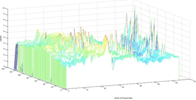
In real market, however, the term structure of spot rates behaves nicer. According to the series of studies by N.L.Liu and her collaborators [25–27], from the term structure of spot rates only two or three factors up to almost 99% are detected when applied a principal component analysis (or its vari-ants), while that of forward rates exhibits more than 10, sometimes 15, or even more factors. Much more straightforward peculiarity is that the sam-ples of the term structure of forward rates often have more humps than those of spot rates.
Figure 1: Typical forward rate movement: EU zero rate
The main aim of the present paper is to propose a new point of view where the humps are understood as a kind of solitons.
The rest of the paper is organized as follows. In section 2.2, we illustrate our idea by a primitive one dimensional example. In section 2.2.1, we present a brief introduction to solitons. In section 2.3, we give a multi-dimensional version of the observation made in section 2.2. We emphasize that a class of affine (quadratic Gaussian) models exhibits multi-soliton shape term struc-tures. Finally in section 2.4, we remark that the solitons appearing in the term structure models are related to a non-linear partial differential equation called KdV equations.
2.2
A primitive example
To explain the idea, we start with a primitive example. Let
P (t, T ) = Ex[exp{−1
2 ∫ T
t
c2|Ws|2ds}|Wt], 0≤ t ≤ T, (2.1)
where W is a 1-dimensional Brownian motion. This formula defines an arbitrage-free bond market, which is a simplest example of the quadratic Gaussian model, and at the same time, an affine term structure model (see e.g.[8]) where we consider |W |2 to be a state variable. In fact, we have an
explicit expression as
P (t, T ) ={cosh(c(T − t))}−1/2 × exp{−c
2tanh(c(T − t))|Wt|
2},
and the (instantaneous) forward rate f (t, T ) = −∂Tlog P (t, T ) is then
ex-pressed as f (t, T ) = c 2tanh(c(T − t)) +c 2|W t|2 2 sech 2 (c(T− t)) , (2.2)
which is an affine function in the state variable. By (2.1), we know that
0 1 2 3 4 5 0 0.5 1 0.05 0.1 0.15 0.2 0.25 0.3 0.35 0.4 0.45 t T-t f(t,T)
Figure 3: A sample path of the forward rate given by (2.2) with W0 = 8,
c = 0.1.
is increasing, and therefore the term structure of spot rates under this model behaves nicely, while one notices that
T 7→ f(t, T )
is a rational function of ec(T−t) and e−c(T −t), which is, what we will call in local terminology, a soliton.
Fig. 4 exemplifies a sample path of the affine forward rate.
2.2.1 Solitons
In general, a traveling wave solution to a non-linear (evolution-type) differen-tial equation is not stable; it collapses from the top. The soliton solutions are exceptions. They have (sometimes more than two) solitary waves=humps, and the humps are quite stable even after the “collisions”. Somehow they behave like particles, and that is why they are called “solitons”.
Mathematically, solitons can be defined as some rational functions of expo-nentials (see [10]). More precisely, it is something like
u(t, x) = f g = ∑ iKie Ait−Bix ∑ iLieCit−Dix , (2.3)
where Ai, Bi, Ci, Di, Ki and Li are constants, and the summations are finite
ones. Here we assume maxiCi ≥ maxiAi and miniCi ≤ miniAi to ensure
the existence of the limits at x → ±∞. If we require the inequality to be strict, then the graph x7→ u(t, x) is hump-shaped. Note that solitons of this definition are stable under summation, multiplication, and differentiations. Note that the forward rate (2.2) in the previous section is a soliton in T or
x = T − t in this sense.
2.3
Affine Term Structure as Multi-Soliton
We generalize the observation made in section 2.2. Let W = (W1,· · · , Wn)
be an n-dimensional Brownian motion starting at x = (x1,· · · xn)∈ Rn, de-fined on a filtered probability space (Ω,F, P, {Ft}), Λ = diag(λ1, λ2,· · · , λn)
with for each λi ∈ R (i = 1, 2, · · · , n), and C ∈ M(n) be a positive definite
matrix. Let P (t, T ) := ehCWt,Wti × Ex [ exp { −1 2 ∫ T t |ΛWs|2ds− hCWT, WTi } |Wt ] . (2.4)
Then {P (·, T )} defines an arbitrage-free bond market with
πt= exp { −1 2 ∫ t 0 |ΛWs|2ds− hCWt, Wti } .
Proposition 5. Under the model (2.4), the forward rate is an n-soliton; a
rational function in e±(T −t)λi, i = 1,· · · , n, of degree at most 2n for any state
Wt. Proof. Let K(t) =− cosh(tΛ)C − 1 2Λ sinh(tΛ), L(t) = 2 sinh(tΛ)Λ−1C + cosh(tΛ), (2.5) and H(t) = K(t)· L(t)−1. (2.6) Note that K0(t) =−1 2Λ 2L(t) (2.7) and L0(t) =−2K(t). (2.8)
We will show that
P (t, T )
={det(L(T − t))}−1/2exph(H(T − t) + C)Wt, Wti}.
(2.9)
By the Feynman-Kac formula,
u(t, x) := E [ exp { −1 2 ∫ t 0 |ΛWs|2ds− hCWt, Wti } |W0 = x ] ,
where x = (x1,· · · xn), satisfies the following differential equation:
∂u ∂t = 1 2∆u− 1 2hΛ 2 x, xiu, u(0, x) = e−hCx,xi, (2.10)
where ∆ is the Laplacian. Note that
P (t, T ) = ehCWt,Wtiu(T − t, W
t). (2.11)
It is well-recognized that the solution u to (2.10) is expressed by
exp (
H0(t) +hH(t)x, xi
)
where H is a symmetric-matrix valued differentiable function satisfying dH dt (t) = 2H(t) 2− 1 2Λ 2 , H(0) =−C, (2.13) and H0 is given by dH0 dt (t) = trH(t), H0(0) = 0. (2.14)
Now we see that H given by (2.5) and (2.6) is the unique solution to (2.13). In fact, by (2.7) and (2.8), we have
H0 = (KL−1)0 =−KL−1L0L−1+ K0L−1 = 2(KL−1)2− 1 2Λ 2 = 2H2− 1 2Λ 2,
and also L(0) = I and K(0) =−C, which imply H(0) = −C. Further, by (2.14), eH0(t) = etr{−12 ∫t 0L0(s)L(s)−1ds} = det{e−12 ∫t 0L0(s)L(s)−1ds} = (det{e∫0tL0(s)L(s)−1ds})−1/2. Since (e∫0tL0(s)L(s)−1ds)0 = L0(t)L(t)−1e ∫t 0L0(s)L(s)−1ds,
we see, by the uniqueness of the matrix-valued first order linear differential equation, that
L(t) = e∫0tL0(s)L(s)−1ds.
Thus we have confirmed (2.9), at the same time (2.11) with (2.12), by which we have
f (t, T ) =− ∂
∂TH0(T − t)
+ ∂
Then, by substituting (2.13) and (2.14), we get f (t, T ) =−trH(T − t) − 1 2h(4H(T − t) 2− Λ2)W t, Wti. (2.15)
We note that the (i, j)-th entries kij and lij of K(t) and L(t) are given by
kij =− cosh(tλi)cij −
1
2δijsinh(tλi), and
lij = 2 sinh(tλi)λ−1i cij + δijcosh(tλi),
and thus they are polynomials in e±tλi. Since
H(t) = K(t)L(t)−1 = K(t) ˜L(t)(det(L(t)))−1,
where ˜L(t) is the cofactor matrix of L(t), we see that each entry of H(t)
is a rational function in e±tλi, i = 1,· · · , n, with degree n. Hence, by the expression (2.15), we have the assertion.
Remark 6. It is known that the forward rates stay positive if π is a strict
supermartingale. In fact, for T1 > T2 we have
Ex[πT1|Ft] < Ex[πT2|Ft]
by the supermartingale property of π, and the formula reads
P (t, T1) = Ex[πT1|Ft] πt ≤ Ex[πT2|Ft] πt = P (t, T2),
meaning that P (t,·) and hence log P (t, ·) is decreasing. This in turn implies that f (t, T ) =−∂T log P (t, T ) is positive.
We give a sufficient condition that ensures the positivity. Since
dπt = πt(−dhCWt, Wti − 1 2|ΛWt| 2 dt + 1 2d[hCWt, Wti]t) =−2hCWt, dWti − trCdt − 1 2|ΛWt| 2dt + 2 2 2|CWt| 2dt,
we see that π is a supermartingale, and hence the forward rates stay positive, if
Λ2− 4C2 > 0
2.4
Remarks on a relation with KdV equation
Let ˜f (t, T ) := f (c2 24t,212T ). Then, we have ˜ f (t, T ) = c 23 tanh (1 2( c 2T − c3 23t) ) +c 2|W t|2 23 sech 2(1 2( c 2T − c3 23t) ) =: v(t, T ) +|Wt|2u(t, T ).By this scale change, the functions u and v satisfy 4∂T∂v = u and
∂u ∂t =−6u ∂u ∂T − ∂3u ∂T3. (2.16)
The equation (2.16) is known as the Korteweg-de Vries equation (KdV equa-tion for short), which describes waves on shallow water surfaces. The KdV equation is mathematically as well as physically quite important in that there are many infinite dimensional symmetries which allow it to have great many explicit solutions including elliptic ones, rational ones, and most importantly in our context, soliton ones.
The relation has been extensively studied, especially by N. Ikeda and S. Taniguchi [14, 15, 33–35]. An extended relation to KP solitons using stochas-tic areas is given in [1].
2.5
Parameterization as a tau function of KP solitons
As we have stated, a tau function τ of the n-soliton solution of the Kadomtsev-Petviashvili equation (KP equation) is expressed by
τ (x1, x2,· · · ) = det(I + G(x1, x2,· · · )), (2.17) with G(x1, x2,· · · ) = (√m imj pi− qj e12(ξi+ξj) ) 1≤i,j≤n , where ξi = (pi− qi)x1+ (p2i − qi2)x2+· · · , i = 1, · · · , n,
Theorem 7. Let P =
(
1
pi−qj )
1≤i,j≤n, and assume that mini,j|pi − qj| is
sufficiently large so that I + P is invertible. Then, if we put A = (I− P )(I + P )−1 and Λ := diag{−12(ξ1 + log m1),· · · , −12(ξn + log mn)}, we have that
(E[eSˆA,Λ(√−1)])−1, where ˆS
A,Λ is defined by (1.13), defines a tau function of
KP solitons. Proof. Since
G = e−ΛP e−Λ,
we have
τ = det(I + e−ΛP e−Λ)
= det e−Λdet(eΛ+ P e−Λ) = det(I + P e−2Λ). On the other hand,
det(cosh Λ + A sinh Λ) = det ( eΛ+ e−Λ 2 + A eΛ− e−Λ 2 ) = 2−ndet{(I + A)eΛ+ (I − A)e−Λ} = 2−ndet{(I + A)eΛ} det
( I + (I + A)−1(I− A)e−2Λ) ) = 2−ndet(I + A)e−12 ∑ (ξi+log mi)det ( I + P e−2Λ ) .
The last equality follows since
A = (I− P )(I + P )−1 ⇐⇒ P = (I + A)−1(I− A).
As we have stated in Remark 1, 2−ndet(I + A)e−12(ξi+log mi) is a trivial factor
and thus by Theorem 2 we have the assertion.
2.6
Reduction to Ikeda-Taniguchi’s construction
As we have discussed in section 1.1.1, we have (1.2) by the reduction of
qj = −pj in (1.7). In this section, we review this from the perspective of
stochastic analysis. We will show that when C− = 0, the expectation of the exponential of the generalized stochastic area is reduced to that of the exponential of the time integral of an Ornstein-Uhlenbeck process, which corresponds to the Taniguchi-Ikeda’s construction (1.8), (1.9) and (1.10) of reflectionless potentials/tau functions of KdV solitons.
Proposition 8. Suppose that A in Theorem 2 is symmetric. Then E[eSˆA,Λ(√−1)] = ( E[e−∫01X A,Λ s ds] )2 etrΛA,
where XA,Λ = h(Λ − AΛA)ξ, ξi and ξ is an Ornstein-Uhlenbeck process on
Rd starting at 0 and satisfying
dξt= Λ
1
2dBt+ ΛAξtdt, (2.18)
with B being an n-dimensional standard Brownian motion.
Proof. We first note the following identity since its right-hand-side also equals
to that of (1.14) with σ replaced by √−1 (see e.g. [22]):
E[e√−1∑lλlSl|W 1] = E[e− ∑ l λ2l 2 ∫1 0{(W l,1 s )2+(Wsl,2)2} ds|W 1].
Then since C+ = A and C− = 0, we have
E[eSˆA,Λ( √ −1)] = ∏ i=1,2 E[e−∑l λ2l 2 ∫1 0(W l,i s )2ds+12hΛ 1 2AΛ12Wi 1,Wi1i] = ( E[e−∑l λ2 l 2 ∫1 0(W l,1 s )2ds+12hΛ 1 2AΛ12W1 1,W11i] )2 .
By applying Itˆo’s formula,
e−∑l λ2l 2 ∫1 0(W l,1 s )2ds+12hΛ 1 2AΛ12W1 1,W11i = e12trΛAe ∫1 0hΛ 1 2AΛ12W1 s,dW1si−12 ∫1 0 |Λ 1 2AΛ12W1 s|2dse−12 ∫1 0h(Λ−AΛA)Λ 1 2W1 s,Λ 1 2W1 si ds. Define Q by dQ dP F1 = e∫01hΛ 1 2AΛ12W1 s,dW1si−12 ∫1 0 |Λ 1 2AΛ12W1 s|2ds.
Then by the Maruyama-Girsanov theorem, we see that W under Q has the same law as ξ of (2.18). This completes the proof.
Remark 3. Note that the variable x appearing in (1.8) is suppressed in the
Remark 4. We note that the 2n-dimensional Brownian motion used to
rep-resent n-solitons in Theorem 2 can be replaced by a 2-dimensional one ir-respective of n. Let W ≡ (W1, W2) be a 2-dimensional Brownian motion
starting at the origin, and set fi(t) := √ n n ∑ l=1 δli1[l−1 n , l n)(t), i = 1, 2,· · · , n, where δji = { 1 i = j, 0 otherwise. Define Si,j+ := ∑ a=1,2 (∫ 1 0 fi(t) dWta ) (∫ 1 0 fj(t) dWta ) , and Si,j− := ∫ 1 0 (∫ t 0 fj(s) dWs2 ) fi(t) dWt1− ∫ 1 0 (∫ t 0 fi(s) dWs1 ) fj(t) dWt2.
We assume that λi > 0 for all i. We shall denote the (i, j) entry of the
matrices Λ12C+Λ 1 2 and Λ 1 2(I + C−)Λ 1 2 by λ+
i,j, and λ−i,j, respectively. Note
that λ−ii = λi. We also assume that either maxl|λl| or kC+k is sufficiently
small to ensure the integrability. Then we have that Ex[e ∑ i,j( √ −1λ− i,jS−i,j+ 1 2λ + i,jS + i,j)](= E x[e ˆ SA,Λ( √ −1)]) = det(cosh Λ + A sinh Λ)−1.
With this identification, it would be possible to obtain another class of τ -function to KP hierarchy by letting n→ ∞ as in [22].
3
Wiener Functionals as Fermions and their
Bosonization via Stochastic Areas
3.1
Introduction
3.1.1 What is done in this section?
As is well-known, the Wiener chaos expansion induces a representation of the Heisenberg algebra, which fact is a keynote of the Malliavin calculus. The
fact that the expansion also induces a representation of Clifford algebra is, as P. A. Mayer pointed out in his book [23], a fact whose significance is not
generally appreciated by probabilists.
In [2], some of the properties of the representation are studied. This section is a continuation of [2], concentrating on Bosonization(s) of the rep-resentation. As a main result, Theorem 17 presents a Bosonization that is
probabilistic in that the map is given by an “integral operator” whose kernel
is given in terms of stochastic areas: roughly, the result is illustrated as ∫
e∑xi×stochastic areas(a Fermion in Wiener space)dµ
= (the corresponding Boson; a character polynomial in (x1,· · · )),
where µ is the two-dimensional Wiener measure and the “stochastic areas” are namely the areas drawn by transformed paths.
The following three observations are the keys to Theorem 17.
1. The representation is unitary (Theorem 12 and Theorem 15) and there-fore the “vacuum expectation value” becomes the standard expectation in Wiener space (Theorem 14).
2. A Fermionic stochastic integral (multi-order stochastic area) decom-poses into “Pfaffian” of (second order) stochastic areas (Lemma 18, a result in [2]), and among the Pfaffian expression, the charge-zero part reduces to “determinant” (Lemma 19).
3. In the representation, the products of second order fermions again be-come orthogonal to each other (Lemma 20).
3.1.2 Why a probabilistic Bosonization is important?
A motivation of the series of studies [1], [2] (and this paper) lies in a prob-abilistic representation of “tau-functions”2. There has been a strong belief
among (a part of) probabilists that there are (hidden) beautiful probabilistic interpretations to special functions such as zeta-, theta-, and tau- functions, and our motivation is in line with these.
According to the results by Sato’s school (see [24] and the references therein), we have roughly
{tau functions} = Bosonization of exp { quadratic forms of Fermions
that form an ∞-dimensional Lie algebra}.
Since we have already at hand fermioninc Wiener functionals, our Bosoniza-tion gives a totally probabilistic representaBosoniza-tion of tau funcBosoniza-tions.
3.1.3 The Organization of the Present Section
Section 3.2 is devoted to a survey on an abstract theory of Fermions and
Bosons, or (the) Clifford algebra and (the) Heisenberg algebra, following
mainly [24]. Section 3.3 is the main part. After introducing a represen-tation of Clifford algebra in Wiener space in section 3.3.1, we will show that it is unitary, and then the vacuum expectation value is realized as the stan-dard expectation with respect to the Wiener measure in section 3.3.2. Then in section 3.3.3 we give a first Bosonization, which is rather algebraic than probabilistic. Finally in section 3.3.4 we shall present our main result and its proof, based on several lemmas.
3.2
Fermions and Bosons
3.2.1 Heisenberg Algebra
Let C ≡ C[x1, x2,· · · ] be the space of all polynomials of infinite variables
x1, x2,· · · , xn,· · · . Define an, a∗n∈ End(C), n ∈ N by
anf =
∂f ∂xn
, a∗nf = xnf. (3.1)
Then, they satisfy the canonical commutation relations: for n, m∈ N, [an, am] = anam− aman = 0, [a∗n, a∗m] = 0, and [an, a∗m] = δnm, (3.2)
where δnm is Kronecker’s delta. Clearly,
C = span{a∗i
1· · · a
∗
in1 : i1,· · · , in∈ N, n ∈ Z+}.
In general, abstract symbols endowed with a multiplication satisfying the relations (3.2) are called Bosons, and the algebra generated by the symbols
with (3.2) defining relations is called the Heisenberg algebra. The above (3.1) can be understood to be constructing a representation of the Heisenberg algebra, where C is the representation space. Namely the algebra is realized as a subalgebra of End(C). We may alternatively call the algebra an H-module if we denote the Heisenberg algebra by H.
If there is an element v in a representation space V such that
V = (a closure of) span{a∗i1· · · a∗inv : i1,· · · , in ∈ N, n ∈ Z+},
then the space is called a Bosonic Fock space, and in this representation
a∗n’s are called creations and an’s are annihilations. It is obvious that C is a
Bosonic Fock space. A symmetric Fock space, which is usually constructed from a separable infinite dimensional Hilbert space H by
⊕∞
n=0Hn⊗sym
is also a Bosonic Fock space in the above sense.
3.2.2 Clifford Algebra
The Clifford algebra Cl is the algebra generated by the symbols ϕn, ϕ∗n,
indexed by half integers n ∈ Z + 1/2, with defining relations
[ϕm, ϕn]+ = ϕmϕn+ ϕnϕm = 0, [ϕm∗ , ϕ∗n]+ = 0, and [ϕ∗m, ϕn]+ = δm+n,0.
The generators are called fermions, and those with negative index are called
creations and the others are called annihilations. It can be easily checked
that
Cl = span{ϕ−i1· · · ϕ−irϕ
∗
−j1· · · ϕ
∗ −jm
: 0 < ir <· · · < i1, 0 < jm <· · · < j1are half integers, and r, m∈ Z+}
as a vector space, and so an irreducible left Cl -module, which is called a
Fermionic Fock space, always takes the form of (a closure of)
span{ϕ−i1· · · ϕ−irϕ
∗
−j1· · · ϕ
∗ −jmv
: 0 < ir <· · · < i1, 0 < jm <· · · < j1are half integers, and r, n∈ Z+}
for an element v in the representation space, which is called a vacuum state. Similarly, an irreducible right Cl -module, which is referred to as a dual Fermionic Fock space, always takes the form of (a closure of)
span{vϕjm· · · ϕj1ϕ
∗ ir· · · ϕ
∗ i1 :
0 < ir<· · · < i1, 0 < jm <· · · < j1are half integers, and r, m∈ Z+}.
An anti-symmetric Fock space, which is usually constructed from a sepa-rable infinite dimensional Hilbert space H by
⊕∞ n=0Hn∧
is also a Fermionic Fock space in the above sense.
3.2.3 Vacuum Expectation Value
Let F be a Fermionic Fock space and F∗ be a dual Fermionic Fock space. For a fixed pair of vacuum states v∗ ∈ F∗ and v ∈ F, define a bilinear form
h·|·i : F∗× F → C by hv∗|vi = 1 and
hv∗ϕ j0 m0· · · ϕj10ϕ ∗ i0r0· · · ϕ∗i01|ϕ−i1· · · ϕ−irϕ ∗ −j1· · · ϕ ∗ −jmvi = {
δi01−i1,0· · · δi0r−ir,0δj10−j1,0· · · δjm0 −jm,0 r0 = r and m0 = m
0 otherwise.
The map is called a vacuum expectation value. We note that
hv∗a|bvi = hv∗|abvi = hv∗ab|vi. (3.4)
The vacuum states are often denoted by vac and an element ofF is by u|vaci or simply by |ui for u ∈ Cl. We also note that by (3.4), the expectation can be denoted by (and understood as) hvac|a|vaci or simply hai for a ∈ Cl.
3.2.4 Bosonization
A representation of the Heisenberg algebra in a Fermionic Fock space can be constructed as follows. Let
Hn :=
∑
j∈Z++1/2
: ϕ−jϕ∗j+n :, n ∈ Z,
1. : a : is linear in a, and all the Fermions within the colons anticommute,
2. : 1 := 1∈ C, and {
: aϕ :=: a : ϕ for ϕ an annihilation, : ϕa := ϕ : a : for ϕ a creation.
Note that for each of the basis in the expression (3.3) of the Fermionic Fock space only finite terms are acting.
One can prove (see e.g. [24] for details) that
[Hm, Hn] = mδm+n,0, m, n∈ Z
so that
an := Hn, a∗n:=
1
nH−n, n ∈ N
satisfies the canonical commutation relations (3.2). With these Bosons, we can construct an isomorphism between the Fermionic Fock space and the Bosonic Fock space C introduced in section 3.2.1. Let
H(x)≡ H(x1,· · · , xn,· · · ) := ∞ ∑ n=1 xnHn, and C[z, z−1] :=⊕l∈ZzlC.
For an integer l, define hl| ∈ F∗ by
hl| = hvac|ϕ1/2· · · ϕ−l−1/2 l < 0 hvac| l = 0 hvac|ϕ∗ 1/2· · · ϕ∗l−1/2 l > 0. Then,
Fact 9 (Bosonization, see Theorem 5.1 in [24]). The map Φ :F → C[z, z−1]
defined by
Φ(|ui) =∑
l∈Z
zlhl|eH(x)|ui, u ∈ Cl, is an isomorphism of vector spaces. Moreover, we have
Φ(Hn|ui) =
{
∂
∂xnΦ(|ui) n > 0
3.2.5 Young Diagrams
A Young diagram is a non-increasing sequence of positive integers (f1, f2,· · · )
all but finite members of which is zero. In a pictorial form, a Young diagram is viewed as a figure in the fourth quadrant of the plane, made up of a number of rows of congruent square tiles, with the rows aligned along their left sides, the first row having f1 tiles, the second row f2 tiles, and so on. The only
requirement is that the number of tiles in a row does not increase when we move down from one row to the next.
Young diagrams have an alternative description. Suppose that Y = (f1, f2,· · · , fr) for r in N is a Young diagram, and let s be the diagonal
width of Y when viewed from the top left-hand corner. We write m1 >
m2 > · · · > ms for the number of tiles lying above the NW-SE
diago-nal line (excluding those straddling the line) in each horizontal row, and
n1n2,· · · , ns for the number of tiles lying below the diagonal line
(exclud-ing those straddl(exclud-ing the line) in each vertical column. Then we write Y = (m1, m2,· · · , ms|n1, n2,· · · , ns) for the Young diagram.
Using this notation, we define the character polynomial of Y to be
FY(x) = det(hmi,nj(x)). Here x = x1, x2,· · · , and hm,n(x) = (−1)n ∑ l≥0 pl+m+1(x)pn−l(−x),
where the pi(x) are defined in e
∑∞
j=1kjxj = ∑∞
j=0pj(x)k
j with p
j(x) = 0 if
j < 0. Here hm,n(x) = Fm+1,1n(x) is the character polynomial corresponding to the hook shaped Young diagram (m + 1, 1n), where 1nstands for the series of n terms (1, 1,· · · , 1).
The following fact plays an important role in our results.
Fact 10 (A characterization of bozonization, see Theorem 9.4 in [24]). The
bosonization Φ is characterized by the following property: the basis vector ϕm1· · · ϕmrϕ
∗ n1· · · ϕ
∗
nr|vaci,
for m1 < m2 <· · · < mr < 0 and n1 < n2 < · · · < nr < 0 of the Fock space
of charge 0 goes over into the character polynomial of the Young diagram of the form Y = ( − m1 − 1 2,· · · , −mr− 1 2| − n1− 1 2,· · · , −nr− 1 2 )
multiplied by the sign (−1)∑ri=1(ni+1/2)+r(r−1)/2.
Here, the meaning of charge will be clarified in section 3.3.1.
3.3
A Probabilistic Bosonization
3.3.1 A Realization of Fermions in Wiener Space
Let (Ω,F , P ) be a probability space, W ≡ (W1, W2) be a two-dimensional real Brownian motion on it starting at the origin, and we set a one-dimensional complex Brownian motion Z = W1+ i W2, and FZ
1 = σ({Zt; t≤ 1}).
We decompose L2[0, 1] = L+⊕ L−, where L+ and L− are mutually
iso-morphic and orthogonal. Let {fi}i≥1 and {gi}i≥1 be orthonormal bases of
L+ and L−, respectively. Let Hl be the closure of the subspace of L2(F1Z)
spanned by ∫ 1 0 ∫ · · · ∫ fm1dZf · · · f fmk1dZf gn1dZf · · · f gnk2dZ;
m1,· · · , mk1 are distinct natural numbers
and so are n1,· · · , nk2,
with the constraint that k1− k2 = l,
where the operation f is defined as follows; for complex semi-martingales
X1,· · · , Xn, ∫ 1 0 ∫ · · · ∫ dX1f · · · f dXn = ∑ σ∈Sn sgnσ ∫ 1 0 ∫ t1 0 · · · ∫ tn−1 0 dXtσ(n)n · · · dXtσ(1)1 ,
where Sn is the n-th symmetric group of permutations. An element of Hl
is said to be of charge l. We set H = ⊕l≥0Hl.
We define bounded operators ψi and ψi∗ acting on H, indexed by
half-integers, as follows; for i > 0,
ψi ( ∫ 1 0 ∫ · · · ∫ fm1dZ f · · · f fmk1dZ f gn1dZf · · · f gnk2dZ ) = (−1)k1+j−1∫1 0 ∫ · · ·∫ · · · f gnj−1dZf gnj+1dZ f · · · ∃j such that i = nj+ 1/2, 0 otherwise,
ψ−i ( ∫ 1 0 ∫ · · · ∫ fm1dZf · · · f fmk1dZ f gn1dZ f · · · f gnk2dZ ) = { 0 ∃j such that i = mj, ∫1 0 ∫ · · ·∫ fidZf fm1dZf · · · otherwise, ψi∗ ( ∫ 1 0 ∫ · · · ∫ fm1dZ f · · · f fmk1dZf gn1dZf · · · f gnk2dZ ) = (−1)j−1∫1 0 ∫ · · ·∫ · · · f fmj−1−1/2dZ f fmj+1−1/2dZ f · · · ∃j such that i = mj + 1/2, 0 otherwise, and ψ−i∗ ( ∫ 1 0 ∫ · · · ∫ fm1dZ f · · · f fmk1dZ f gn1dZf · · · f gnk2dZ ) = 0 ∃j such that i = nj + 1/2, (−1)k1∫1 0 ∫ · · ·∫ · · · f fmk1dZ f gidZf gn1dZf · · · otherwise.
The following is obtained as a special case of the result in [2].
Proposition 11 ([2]). Let C be the algebra generated by {ψm, ψn∗; m, n ∈
Z + 12}. (i) Then C is a Clifford algebra ; i.e.
[ψm, ψn]+= 0, [ψm∗, ψn∗]+= 0, and [ψm, ψ∗n]+ = δm+n,0.
(ii) The set ψ−m1· · · ψ−mkψ−n1∗ · · · ψ−nl∗ (1) is an orthogonal basis of H.
Proposition 11 above states thatH is an irreducible Cl-module. We may identify ψ−m1· · · ψ−mkψ−n∗ 1· · · ψ−n∗ l|vaci = ψ−m1· · · ψ−mkψ ∗ −n1· · · ψ ∗ −nl(1), for 0 < mi, nj ∈ Z + 12, i, j ∈ N, and so on.
3.3.2 The Vacuum Expectation in Wiener Space
Lemma 12. For k, l∈ N with l = k + 1, if a half-integer i satisfies any one
of the following conditions (a),(b); a) ms+1 < i < ms with 1≤ s < s+1 ≤ k;
in this case we rename the subscripts, ns0 = m0s0 if 1 ≤ s0 ≤ s, ms0 = m0s0+1
if s + 1≤ s0 ≤ k and i = m0s+1 otherwise; b) i = ms, then
( ψ−i, ψ−m1· · · ψ−mkψ ∗ −n1· · · ψ ∗ −nl(1), ψ−m0 1· · · ψ−m0k+1ψ ∗ −n1· · · ψ ∗ −nl(1) ) H =(ψ−m1,· · · ψ−mkψ ∗ −n1· · · ψ ∗ −nl(1), ψi∗ψ−m0 1· · · ψ ∗ −m0 k+1ψ ∗ −n1· · · ψ ∗ −nl(1) ) H, (3.5)
where 0 < m1,· · · , mk, m01,· · · , m0k+1, n1,· · · , nl runs the half-integers Z +12.
Proof. case a). Suppose i = m0u with 1≤ u ≤ k + 1. Left hand side of the equation (3.5)
=(ψ−iψ−m1· · · ψ−mkψ−n∗ 1· · · ψ−n∗
l(1),
ψ−m0
1· · · ψ−m0u−1ψ−iψ−m0u+1· · · , ψ−m0k+1ψ
∗ −n1· · · ψ ∗ −nl(1) ) H = (−1)u−1(ψ−iψ−m1· · · ψ−mkψ−n∗ 1· · · ψ ∗ −nl(1) ψ−iψ−m0 1· · · ψ−m0u−1ψ−m0u+1· · · ψ−m0k+1ψ ∗ −n1· · · ψ ∗ −nl(1) ) H = 1× (−1)u−1, and
Right hand side of the equation (3.5) =(ψ−m1· · · ψ−mkψ−n∗ 1· · · ψ−n∗ l(1), ψi∗ψ−m0 1· · · , ψ−m0u−1ψ−m0uψ−m0u+1· · · ψ−m0k+1ψ ∗ −n1· · · ψ ∗ −nl(1), ) H = (−1)u−1(ψ−m1· · · ψ−mkψ∗−n 1· · · ψ−nl(1), ψ−m0 1· · · ψ−m0u−1ψ ∗ iψ−m0uψ−m0u+1· · · ψ−m0k+1ψ ∗ −n1· · · ψ ∗ −nl(1)i ) H = (−1)u−1× 1. Thus (3.5) holds.
case b). Suppose i = ns with 1≤ s ≤ l + 1.
Left hand side of the equation (3.5) =(ψ−iψ−m1· · · ψ−mkψ−n∗ 1· · · ψ−n∗ l(1), ψ−m0 1· · · ψ−m0k+1ψ ∗ −n1· · · ψ ∗ −nl(1), ) H = (−1)s−1(ψ−m1· · · ψ−ms−1ψ−iψ−msψ−ms+1· · · ψ−mkψ−n∗ 1· · · ψ ∗ −nl(1), ψ−m0 1· · · ψ−m0k+1ψ ∗ −n1· · · ψ ∗ −nl(1) ) H = (−1)s−1× 0 = 0.
The above lemma describes adjoint operators of Fermions (ψi)adj. and
(ψ∗i)adj. ;
Theorem 13. We have that
(ψi)adj.= ψ−i∗ , and (ψi∗)
adj.= ψ
−i (3.6)
for i∈ Z + 12.
As a corollary, we show that the vacuum expectation introduced in section 3.2.3 is expressed by the usual expectation in Wiener space:
Theorem 14. We have
hu|vi = E[uadj.(1)v(1)], (3.7)
for u, v ∈ Cl. Proof. We put u = ψm1· · · ψmrψ ∗ n1· · · ψ ∗ ns, v = ψm01· · · ψm0r0ψ ∗ n01· · · ψ∗n0 s0 , where m1 > · · · > mr > 0, n1 > · · · > ns > 0, 0 < m01 < · · · < m0r0, and
0 < n01 <· · · < n0s0, then E[uadj.(1)v(1)] = E[uv(1)] = E [ ψm1· · · ψmrψ ∗ n1· · · ψ ∗ ns ∫ 1 0 ∫ · · · ∫ fm01−1/2dZ f · · · f fm0r0−1/2dZf gn01−1/2dZf · · · f gn0s0−1/2dZ ] = (−1)js−1E [ ψm1· · · ψmrψ∗n1· · · ψ ∗ ns−1 ∫1 0 ∫ · · ·∫ · · · f fm0js−1−1/2dZf fm0js+1−1/2dZf · · · ] ∃js ∈ {1, · · · , r0} such that m0js = ns 0 otherwise = · · · = (−1) ∑s k=1k−s− ∑s l3=2 ∑s−1 l2 ∑l2 l1=1δ{jl1<jl3} ×∏s α=1,jα∈{1,··· ,r0}δ−m0jα+nα ∏r β=1,jβ∈{1,··· ,s0}δmjβ−n0β r = s0, r0 = s 0 otherwise = { ∏s α=1,jα∈{1,··· ,r0}δ−m0jα+nα ∏r β=1,jβ∈{1,··· ,s0}δmjβ−n0β r = s 0, r0 = s 0 otherwise = hu|vi. 3.3.3 A Bosonization Let Hn := ∑ j∈Z++1/2 : ψ−jψ∗j+n :, n ∈ Z.
We also have the following as a corollary to Theorem 14;
Theorem 15. We have
Proof. We proof only when k > 0. Hkadj. = ( ∑ j∈Z++1/2 : ψ−jψj+k∗ : )adj. = ( ∑ j∈Z++1/2 ( ψ−jψj+k∗ − δk,0θ(j <−k) ))adj. = ∑ j∈Z++1/2 ( ψ−jψj+k∗ )adj. − ∑ j∈Z++1/2,j<0 δk,0θ(j <−k) = ∑ j∈Z++1/2 ψ−j−kψj∗− ∑ j∈Z++1/2,j<0 δk,0θ(j <−k) = H−k.
The following is a direct consequence of Fact 9, Fact 10, Lemma 12, and Theorem 15.
Corollary 16. The map
Ψ :H → C[x1, x2,· · · ], given by Ψ(X) =∑ l∈Z zlE[eHadj.(x) ladj.(1)X], X ∈ H, or equivalently Ψ(X) = ∑l∈ZzlE[leHX] or Ψ(X) = ∑ l∈Zz
lE[ladj.(1)eHX],
where l(1) = ψ∗l+1/2· · · ψ∗−1/2(1) for l < 0, 1 l = 0, ψ−l+1/2· · · ψ−1/2(1) for l > 0, is a Bosonization; Ψ ( Hnu(1) ) = ∂ ∂xnΨ ( u(1) ) n > 0 −nx−nΨ ( u(1) ) n < 0,