東京海洋大学学術機関リポジトリ　TUMSAT-OACIS

TUMSAT-OACIS Repository - Tokyo University of Marine Science and Technology (東京海洋大学)

Research on optimization of container ship's

bracket

学位名

修士(工学)

学位授与機関

東京海洋大学

学位授与年度

2020

Master’s Thesis

RESEARCH ON OPTIMIZATION OF

CONTAINER SHIP’S BRACKET

September 2020

Graduate School of Marine Science and Technology

Tokyo University of Marine Science and Technology

Master’s Course of Marine Technology and Logistics

Master’s Thesis

RESEARCH ON OPTIMIZATION OF

CONTAINER SHIP’S BRACKET

September 2020

Graduate School of Marine Science and Technology

Tokyo University of Marine Science and Technology

Master’s Course of Marine Technology and Logistics

Abract

With the development of international trade in recent years, container ship has become the main force of ship transportation because of its high efficiency, convenience, safety and reliability. Container transportation greatly reduces the transportation cost, which makes the container transportation get a high-speed development. Moreover, because the large container ship can reduce the cost, the development of global economic integration, the widening of Panama Canal, and higher security and other factors, the large-scale container ship has become the development trend of the ship type. Therefore, the research on the structure of large container ships has a very important theoretical significance and application value, which attracts more and more attention of ship scientists, especially the analysis of the strength of the cabin section and the strength of the whole ship structure is a hot issue in recent years. Aiming at the strength problem of large container ships and combining with the actual situation, this paper has carried out the following work:

Firstly, the principle of calculating grillage stress by finite element software is studied, and the provisions of the code for classification of steel seagoing vessels in the aspects of finite element model, definition of boundary conditions, types and calculation methods of design loads, and evaluation criteria of structures are understood. In addition, the design load calculation and structural finite element modeling technology of container ship are studied, and a 24000DWT multifunctional container ship is selected for three-dimensional modeling building. Five typical working conditions are selected in the code to calculate the structural loading and evaluate the yield strength. In order to consider the role of the bracket plate in the joint structure, several models are established to analyze the stress of each joint structure with and without bracket plate. The comparison of the stress results of the two cases shows that the existence of the bracket plate improves the stress concentration at the joint of the bulkhead girder and the platform truss, and enhances the bending characteristics of the truss.

In order to improve the stress concentration of the bracket plate joint structure, the method of changing the bracket plate material and changing the bracket plate size is carried out in this paper. In the calculation of changing materials, six kinds of high-quality carbon structural steels and three kinds of alloy structural steels were selected. The results show that only changing the material of the bracket plate, whether it is high-quality carbon structural steel or alloy structural steel, has only a slight impact on other hull members. In the calculation of changing the size, the thickness of triangle bracket plate, the thickness of rectangular bracket plate and the elimination of bracket flange are adopted respectively, and the influence of bracket plate size on the stress of other members is analyzed in six groups. According to the calculation results of the ship, it can be concluded that the thickness of the two kinds of brackets can be reduced and the flange of the brackets can be canceled within the allowable range of the code.

In this paper, the idea and method of the structural analysis of the bracket plate joint are put forward, which can provide reference for the similar structural analysis and optimization design.

Contents

1. Introduction... 1

1.1 Background, purpose and significance...1

1.2 Purpose and significance of the paper...2

1.3 Main research contents of this paper...3

2 Finite element technology and MSC.Patran & Nastran software... 5

2.1 Development of finite element technology... 5

2.2 Concept of finite element analysis... 6

2.3 Theory of finite element method...9

2.4 MSC.Patran & Nastran software...16

2.5 Summary of this chapter... 17

3. Provisions of direct calculation by CCS... 18

3.1 Establishment of finite element model of ship based on CCS code...18

3.2 Load calculation and load condition... 19

3.3 Boundary conditions... 27

3.4 Strength assessment...28

3.5 Summary of this chapter... 29

4. Direct calculation and analysis of yield strength of real ship...30

4.1 Basic information of real ship model... 30

4.2 Boundary conditions and Model grouping...33

4.3 Calculation condition and Loading mode... 37

4.4 Load application...39

4.5 Calculation and analysis...40

4.6 Summary of this chapter... 45

5. Optimization design of bracket plate for real ship... 46

5.1 structural design of stress concentration area...46

5.2 The extent of bracket plate impact on hull members... 47

5.3 Influence of different materials of bracket plate on other component... 51

5.4 Influence of changing bracket size on other component...53

5.5 Summary of this chapter... 56

6.Conclusion and prospect... 57

6.1 Conclusion...57

6.2 Prospect of future work... 58

Acknowledgement...59

1. Introduction

1.1 Background, purpose and significance

In today's world, as the main means of transportation of bulk commodities, ships play a leading role in various modes of transportation due to their advantages of large cargo carrying capacity and low transportation cost. However, if there is an accident when the ship is sailing on the sea, it will not only cause casualties, but also cause huge economic losses such as cargo dumping into the sea, ship sinking, as well as a large number of deaths of marine organisms, destruction and pollution of the marine environment, and other huge ecological damage, the loss is very huge. Therefore, the safety of ship structure plays an important role in ship design, which is the most concerned problem of designers, builders and operators. According to the research, the main reason for the high incidence of accidents is the fatigue failure of the hull.

In fact, the fatigue damage of ships can be observed. Generally, before the serious fatigue failure of the ship, there will be very small cracks in many components of the ship. However, due to the huge number of ship components, it is impossible to carry out comprehensive and detailed fatigue crack inspection and maintenance, which is a great test for human and material resources, and precisely because of this, it is impossible to deal with the initial cracks timely and properly, and the initial cracks will become larger and larger in the long-term navigation process, eventually leading to uncontrollable serious fatigue damage.

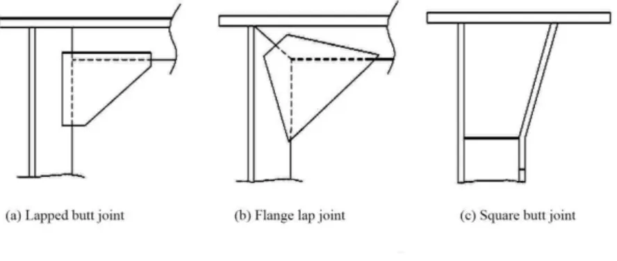
Some studies have shown that the initial cracks are generated first in some joint structures. In 1978, Charles R. Jordan analyzed 490230 nodes in 12 structural nodes of 50 ships, and the number of damaged nodes was 3307. Among them, 2227 nodes were damaged due to cracks. Among them, 50.97% of the nodes were damaged at the bracket joints, and the number was 1135.In 1980, Charles R. Jordan did a similar work. He made statistics on node damage of 36 ships, including 117374 nodes in total and 3555 nodes in damage. 74.2% of the total number of joint failures occurred in the bracket joints, the number of which was 2673. The total number of nodes in the two analyses of Charles R. Jordan is 607584, of which the total number of bracket nodes is 102598. In the statistical results of Charles R. Jordan, the three types of bracket nodes with the most damage are shown in Figure 1.1(1). Among them, 1344 were damaged in the first form, 601 in the second and 433 in the third.

Figure 1.1(1) Three types of bracket plate with more damages

In conclusion, because ship components are mainly connected by nodes, the mechanical properties of ship nodes can directly affect the carrying capacity of the ship. The main structural form of the ship joint is the bracket plate structure, and the ship damage mainly occurs on the ship bracket joint. The fundamental method to improve the fatigue damage of the ship is to reduce the tensile stress at the joint, and the structural form is to improve the fatigue life and reduce the stress concentration. In this paper, based on this background, with a comprehensive understanding of the mechanical characteristics of the bracket joint structure, the optimization analysis of the ship's bracket structure is carried out to obtain the bracket structure type which can improve the stress concentration.

1.2 Purpose and significance of the paper

In addition to the function of convenient assembly, the bracket plate also has the function of strengthening the joint stiffness and strength. Therefore, the bracket plate is the most commonly used connecting component in the ship structure. In addition, the bracket plate structure also has a certain strengthening effect on the fixation of the end of the skeleton. The bracket plate reduces the discontinuity of the ship component and connects the ship frame into a whole. However, the bracket plate structure bears a large reaction force, bending moment and torque. In the code for classification of Chinese steel sea going ships, the definition of the bracket plate is: the additional component used to increase the strength of the joint of two components. In the code, it is also emphasized that in the process of designing the bracket plate, not only the connection strength of the bracket plate, but also the factors such as the production process and the utilization rate of materials should be considered. Therefore, the designer of the bracket plate should consider these issues comprehensively.

LR, ABS and other classification society codes have some provisions on node structure. For example, in order to minimize the stress concentration at the joint, the end of the bracket plate should have a larger toe angle, the bracket plate should be arc-shaped as far as possible, and the arm length of the bracket plate represented by the web length of the member should not be greater than the smaller height of the connected member, etc. In

parameters of the bracket plate have clear provisions; if one side of the bracket plate is the main member and the other side is the secondary member, the form of the diagonal toe has very detailed provisions.

Although there are some regulations for all kinds of brackets in the code, the structural form of brackets still has a lot of room for improvement. The stress of the bracket plate is very complex, and the stress magnitude and frequency of the stress have great changes, so it is difficult to carry out accurate theoretical analysis on the stress of the bracket plate. When the ship is sailing on the sea, the external load of the bracket plate changes all the time. In this case, the two toe ends of the bracket plate are prone to stress concentration. When it is serious, it will produce structural hard points, which will lead to the damage of the bracket plate, and finally cause the ship damage and other serious consequences mentioned above. The strength analysis of the bracket plate structure can not only focus on the ship's bracket plate structure, but also on the strength analysis of the components connected with the bracket plate, because only a certain degree of understanding of the stress condition of the connecting structure can more accurately analyze the tension, compression, shear and other stress conditions of the bracket plate, and fully understand the final failure mode of the bracket plate. When the bracket plate is compressed or sheared, or the combination of compression and shear, the limit point of the bracket plate is the buckling point. When the bracket plate is under the tensile action, the limit point of the bracket plate is the yield point, and the bracket plate is the thin plate, and the yield strength is greater than the buckling strength. This is a problem to be noted in the calculation process.

In the past, due to the limitation of calculation method and ability, there were two main methods to calculate the structural stress of ship's bracket plate joint. One is to directly build the bracket plate joint structure in the whole ship finite element model. In this case, if we consider the stress concentration at the ship joint structure, we need to refine the mesh at the bracket plate joint structure, which will greatly increase the grid amount of the whole ship, and affect the mesh quality of the whole ship, will greatly extend the calculation time of the whole ship, and will affect the calculation results of the whole ship. The other method is to make artificial equivalence to the boundary conditions near the bracket plate joint structure, which will lead to large errors.

In view of the above requirements, this paper will carry out a comprehensive mechanical analysis of the bracket plate joint structure and the components connected with the bracket plate structure, and have a detailed and comprehensive understanding of the mechanical characteristics of the bracket plate joint structure and the components connected with the bracket plate joint structure. On this basis, the ship's bracket plate joint structure is optimized to improve the stress concentration of the ship's bracket plate joint structure. This work not only has the theoretical innovation significance, but also has the important engineering significance.

1.3 Main research contents of this paper

In this paper, the problem of joint stress concentration in a ship's cabin model is studied as follows:

(2) In the second chapter, the finite element theory and technology, MSC PATRAN ship modeling software and NASTRAN post-processing analysis software are introduced

(3) In the third chapter, the main steel ship classification codes are introduced and analyzed in detail, which are the aspects of finite element model, boundary condition definition, design load type and calculation method, structure evaluation criteria, etc.

(4) In the fourth chapter, according to the requirements of the code, a part of the model of 24000DWT multi-purpose container ship's parallel midship section is established and its strength is calculated.

(5) In the fifth chapter, the research on the optimization of the material and size of the bracket are carried out, and the stress concentration of the bracket joint structure itself and the adjacent structure are also considered.

(6) The sixth chapter summarizes the work of the whole paper,and puts forward the prospect of the future work.

2. Finite element technology and MSC.Patran

& Nastran software

2.1 Development of finite element technology

The basic formation of the finite element method can be traced back to the 1950s. The basic idea comes from the principle of matrix structure method of solid mechanics and engineers' intuitive judgment of structural similarity. In the field of engineering technology, we often encounter two kinds of typical problems. One kind of problem is called discrete system. The general object is the combination of finite known elements. In general, the discrete system has analytical solutions. But when solving some very complex discrete systems, that is to say, when there are many known elements, it still depends on computer technology to solve the problem. Another kind of problem is called continuous system. The general object is composed of infinitely many infinitesimal elements. In order to solve this kind of problem, we can only establish the basic equations that all elements must follow. However, in view of the limitation of boundary conditions, we can only solve a few simple problems accurately, and most practical engineering problems cannot get proper solutions definitely. Mathematicians and engineers have been exploring the problems that cannot be solved in the above two typical problems, and put forward many approximate methods. In this exploration, the finite element method came into being.

The original intention of the development of finite element is to complete the structural analysis of aviation equipment by computer. After that, finite element method has been widely used in the field of mechanical engineering, civil engineering and other complex structural systems. In fact, many engineering problems can be simplified to solve the control equations with given boundary conditions. Generally, only a few problems with relatively simple equations and very regular boundaries can get accurate analytical solutions. In most engineering and technical problems, the geometry of the structure is relatively complex, with nonlinear characteristics and non-standard boundaries, Generally, there is no analytic solution to this kind of problems. There are two ways to solve this complex problem. The first way is to simplify the equations and boundary conditions, so that they can be solved analytically. But not every problem can be solved by this way, because too much simplification may lead to wrong solutions. The other way is to use mechanics and modern mathematics On the basis of theory, the numerical simulation technology is used to get the numerical solution that meets the engineering requirements.

In the field of engineering technology, numerical simulation methods are often used: finite difference method, discrete element method, boundary element method and finite element method, but in these methods, the finite element method is the most practical and therefore the most widely used. The foundation of the finite element method is the solid flow variational principle. The basic steps of the finite element method are as follows: first, the structures involved in the analysis are separated into many elements; second, the material properties, boundary conditions and loads are given in the analysis; third, the corresponding linear and nonlinear equations are solved, and the results of stress, strain and

displacement are obtained through calculation; fourth, the calculation results are finally displayed by graphic technology 。 At present, the analysis function of the popular commercial finite element program basically covers all engineering fields, and it is also quite convenient to use. General engineers can master and carry out the analysis and calculation of practical projects in a short time, so it is popularized.

2.2 Concept of finite element analysis

Finite element method: the solution area is composed of many small interconnected elements at the nodes. The model gives the approximate solution of the basic equation in pieces. Because the elements can be divided into different shapes and sizes, it can well adapt to complex geometry, complex material characteristics and complex boundary conditions.

Finite element model: it is an ideal mathematical abstraction of real system. It is composed of some simple shape elements, which are connected by nodes and bear certain load.

Finite element analysis: it is to simulate the real physical system (geometry and load condition) by using the method of mathematical approximation. By using simple and interactive elements, a finite number of unknowns can be used to approximate the real system of infinite unknowns.

The discretization of structure is the core idea of finite element calculation. The so-called discretization is to discretize the actual structure into a combination of finite elements in an imaginary way. Therefore, the analysis of these actual structures can be replaced by the analysis of the discrete combination, which solves many complex practical engineering problems that cannot be solved in theory. In short, the finite element method is to discretize the structures to be analyzed and then use the basic mechanical theoretical equations to solve them.

Another important feature of the finite element method is that the approximate function on the element is used to represent the unknown field function on the whole solution domain. This kind of approximate function is generally expressed by the value of unknown field function and its derivative at each node of each element and the corresponding interpolation function. Then the value of the unknown field function and its derivative at each node of each element becomes a new unknown quantity, so that a continuous infinite degree of freedom problem is transformed into a discrete finite degree of freedom problem. By solving these unknown quantities, the approximate value of the internal field function of each element can be obtained through the interpolation function, and the approximate value of the whole solution domain can be obtained. It can be seen from the above that when the number of elements or the degree of freedom of the element or the accuracy of the interpolation function increases, the accuracy of the approximate solution will also increase, and when the element reaches the convergence condition, the approximate solution may

actual shape of the structure to be analyzed and the actual working conditions during the analysis. The purpose of this step is to provide input data for the subsequent numerical calculation. Structural discretization is the central task of finite element analysis, which is embodied in mesh generation in finite element software. In addition, it also needs to deal with such problems as simplification of structural form, definition of element characteristics, numbering sequence of elements, quality inspection, establishment of geometric model and definition of boundary conditions. Modeling is the foundation of the whole finite element. Firstly, the finite element mesh is the source of the original data of the whole finite element analysis, so the error of the original data will directly affect the accuracy and convergence of the calculation results. Secondly, the size of the finite element mesh will directly affect the requirements of the computer hardware, so it is necessary to establish a finite element model that can not only ensure the accuracy of the results, but also not too much calculation, so that the computer storage requirements are too high. Thirdly, in general engineering projects, the geometric structure and actual working conditions of the structure are quite complex, and the modeling time almost accounts for 2 / 3 of the whole finite element analysis time, so we should strive to establish the appropriate finite element model in the first time.

2.Calculation phase. This stage is the core stage of finite element analysis, which is mainly for numerical calculation, and is automatically completed by the finite element analysis software on the computer. There are three main data needed in this stage: first, node number, coordinate value, etc. The second is the number of the element and the node number of the constituent element, the elastic modulus, Poisson's ratio, density, etc., the cross-sectional area, inertia moment, etc., the physical characteristic value of the element and the relevant geometric data, etc. The third is displacement constraint data, load condition data, thermal boundary condition data and other boundary data.

3.Post processing stage. In this stage, the calculation results of the finite element analysis software are processed to a certain extent, and displayed in a certain way, so that the analysts can have an intuitive understanding of the rationality about structural design and the quality of structural performance.

2.3 Theory of finite element method

2.3.1 The fourth strength theory and Von-Mises yield criterion

The fourth strength theory holds that the specific energy of shape change is the main factor causing yield, that is, no matter what stress state, as long as the specific energy of shape change reaches a certain limit value related to the material properties, the material will yield. The theoretical formula of strength is:

σ = (2-1)

Among them, , , are the three principal stresses on the main plane. Plastic materials such as steel follow the fourth strength theory.

The Mises yield criterion is: under certain deformation conditions, when the equivalent stress of a point in the stressed object reaches a certain value, the point begins to enter the plastic state. Its physical meaning is: under certain deformation conditions, when the elastic potential energy (also known as elastic deformation energy) changed by the unit volume shape of the material reaches a certain constant, the material will yield. The strength theoretical formula is the same as (2-1). In the post-processing of finite element software, "von Mises stress" is commonly called Mises equivalent stress, which follows the fourth strength theory of material mechanics.

=

=

-=

Among them, , is the element direct stress, N/ . is the element shear stress, N/ .

The von Mise equivalent stress formula defined in the specification can be obtained by substituting formula (2-1):

=

-2.3.2 Theory of finite element

In recent years, due to the construction of new ships, the large-scale of ships and the rise of the development of offshore platforms, new structures and materials are emerging constantly. The buckling, elastic-plastic failure, fatigue and fracture of ship structures are proposed, which forces us to find new and effective methods for the analysis of Ship

Structures. Moreover, with the development of computer software and hardware technology, it is possible to divide the local structure of the ship or even the whole ship into finite elements for analysis. The strength analysis of the ship structure has a revolutionary breakthrough since then. The whole hull structure is discretized into a finite element which can accurately simulate its load-bearing mode and deformation. For the main structural members, according to their stress conditions, they are expressed by membrane, rod, plate, shell and beam elements. In this way, the micro details of the hull structure can be described in detail, and the coordination relationship and changes among various components can be truly expressed. Through large-scale finite element software analysis and solution, the actual deformation and stress of each concerned component or area can be calculated. This method is the most accurate and perfect method of hull strength analysis at present. It is also the most accurate structural analysis method for predicting the response of the structure to the load in the rational structural design.

The steps of finite element method to calculate structural stress are as follows:

(1) Discretization of structure: according to the requirements of specific structure form and calculation accuracy, the structure is divided into a certain number of units, the structure coordinate system is established and the units and nodes are numbered. Generally speaking, the node and boundary of the element should be placed in the place where the structural geometry, load and material properties are abrupt, and the narrow triangle element should be avoided, because the stress obtained by the triangle element is the average stress, while the narrow triangle element can not reflect the real stress state of the structure in this place.

(2) Calculate the stiffness matrix of the element.

(3) Calculate the total stiffness matrix of the structure: the sub matrix of the obtained stiffness matrix of each element is seated according to the number of its subscript to form the total stiffness matrix.

(4) Establish the external force matrix: transfer the distributed load of the element to the relevant nodes one by one to obtain the equivalent node force, and then add the external force directly acting on the nodes to obtain the node external force matrix.

(5) Constraint processing: constraint processing is performed according to the constraint conditions of the structure.

(6) Solve node displacement: solve the structural node balance equation after constraint treatment, and get the node displacement.

(7) The average stress of the element can be calculated. If necessary, the main stress and direction of the element can also be calculated for analysis. The stress at the element node can be obtained by averaging the stress of adjacent elements. When there are enough elements (the mesh is dense enough), the calculated stress is accurate enough.

In the hull structure, the most commonly encountered is the rectangular grid structure. Next, take the rectangular grid as an example to illustrate the displacement function, element strain and stress, element stiffness matrix and structure stiffness matrix, external

origin. Obviously, this coordinate system is the unit coordinate system, so the coordinates of nodes are i (- a, - b), j (a, - b), m (a, b), p(- a, b).

Figure2.3(1) Rectangle plane element

(1) Displacement function

Each node of the rectangular plane element has two displacements u, V, so four nodes have eight displacements. They constitute the node displacement matrix of the element{δe}_,

and have the corresponding node moment matrix {Fe} _{caused by displacement, as}

follows:

(2-4)

Now the displacement function is introduced, which will be determined by the displacement of 8 nodes，so it's written as:

xy a y a a a y x v xy a y a x a a y x u x 7 8 6 5 4 3 2 1 ) , ( ) , (         (2-5) After substituting the coordinates of four nodes into formula (2-5), can get

} a ]{ A [ } δ { 1 8 8 8 1 8 e     (2-6) Where, (2-7)

From equation (2-6), can get {_a}_[_A]1{δe}_{, so} } δ ]{ [ } δ { ] ][ [ } ]{ [ } { 1 8 e 8 2 e 1 1 2      H a  H A  N d (2-8)

Where [N] is displacement matrix:

] [ ] [N  N_i N_j N_m N_p (2-9) Where， (2-10)

The displacement function obtained above is a quadratic function of coordinates x, y, but it is still a primary function on the boundary of element,

Therefore, the displacement of the boundary is linear, so that the boundary of two adjacent elements still fit in the deformation, so that the moment shape element is the coordination element.

(2) Element strain and stress

(2-11)

Where [B] is geometric matrix:

] [ ] [B  B_i B_j B_m B_p (2-12) Where, (2-13)

From the physical equation, the stress of any point in the element is

} δ ]{ [ } δ ]{ ][ [ } σ { 1 8 e 8 3 e 1 3  D B  S  (2-14)

Where [D] is the elastic matrix and [S] is the stress matrix:

] [ ] [S  Si Sj Sm Sp                2 μ 1 0 0 0 1 μ 0 μ 1 μ 1 ] [D E ₂ (2-15) Where,

                                                                                                   y) (b μ x) (a μ y) (a x) μ(b x) μ(a y) (b ) μ ab( E ] [S y) (b μ x) (a μ y) (a x) μ(b x) μ(a y) (b ) μ ab( E ] [S y) (b μ x) (a μ y) (a x) μ(b x) μ(a y) (b ) μ ab( E ] [S y) (b μ x) (a -μμ(b y) (a x) x) μ(a y) (b ) μ ab( E ] [S p m j i 2 1 2 1 1 4 2 1 2 1 1 4 2 1 2 1 1 4 2 1 2 1 1 4 2 2 2 2 (2-16)

It can be seen that the stress at any point in the element is a linear function of coordinates. For the element center, x = y = 0 is substituted into the above formula to obtain the stress matrix of the element center.

(3) Element stiffness matrix and structure stiffness matrix

The stiffness matrix of rectangular element can be derived by the principle of virtual work just like that of triangular element. After substituting [B] in formula (2-12) and [D] in formula (2-15),can get

                pp pm pj pi mp mm mj mi jp jm jj ji ip im ij ii e K K K K K K K K K K K K K K K K K ] [ 8 8 (2-17) The submatrix is

                                                                                                   f c g c c g c f Et K f c g c c g c f Et K f c g c c g c f Et K f c g c c g c f Et K f c g c c g c f Et K K f c g c c g c f Et K K f c g c c g c f Et K K pj pi mj mi pm ji pp jj mm ii 1 2 2 1 2 1 3 3 1 2 1 3 3 1 2 1 2 2 1 2 1 3 3 1 2 1 2 2 1 2 1 2 2 1 2 2 2 μ 1 ] [ 2 2 μ 1 ] [ 2 2 μ 1 ] [ 2 2 μ 1 ] [ 2 2 μ 1 ] [ ] [ 2 2 μ 1 ] [ ] [ 2 2 μ 1 ] [ ] [ (2-18) Where, 8 μ 3 1 , 8 μ 1 , 4 μ 1 , 3 , 3 1 2 3         c c c b a g a b f (2-19) Because T ji ij K K ] [ ]

[  , the other submatrixes are not written separately.

After the submatrix of the element stiffness matrix is obtained, the submatrix of the element stiffness matrix can be set according to its subscript number to form the structure stiffness matrix [K]. Thus, the equilibrium equation of the joint force of the structure is established: } { } δ ]{ [K  P

Where { δ } is the displacement matrix of structural node and {P} is the external force matrix of structural node.

(4) External load displacement

The nodal force matrix {P} of the structure includes the equivalent nodal force of the distributed force on the element. For the rectangular element, such as the force distributed uniformly in the element, and the resultant force is Q, the equivalent nodal force of the distributed force is derived from the virtual work principle.

4 Q P P P Pi  j  m p  (2-20)

(5) Coordinate transformation

For some structures, the coordinate system of the element is not necessarily consistent with the direction of the structure system after the element division, so the coordinate transformation is needed.

In the plane problem, the relation of coordinate transformation is as follows:

α y α x y α y α x x cos sin sin cos     (2-21)

Where x,y is the element coordinate, x, y is the structure coordinate, and α is the angle from ox to ox clockwise. So the coordinate transformation matrix is

       α cos α sin sinα -α cos ] [t (2-22)

And the following coordinate transformation relations of node displacement, node force and external force are as follows:

} ]{ [ } { }, ]{ [ } { }, δ ]{ [ } δ { e _{ T} e _Fe _{ T F}e _Pe _{ T P}e _(2-23) Where,              t t t t T 0 0 ] [ (2-24)

The coordinate transformation relation of element stiffness matrix is

T ij ij T e e t K t K T K T K ] ][ ][ [ ] [ ] ][ ][ [ ] [   (2-25) After the coordinate transformation of node displacement, element stiffness matrix and external force of node, the balance equation of node force in the structural coordinate system can be formed, or the total stiffness matrix of the structural coordinate system can be obtained. The total stiffness matrix can be constrained to solve the node displacement.

2.4 MSC.Patran & Nastran software

MSC.Patran is an integrated parallel frame finite element pre-processing, post-processing and analysis simulation system. Patran was first developed by NASA. It is a well-known parallel frame finite element pre-processing and analysis system in the industrial field. Its open and multi-functional architecture can integrate engineering design, engineering

reliability and excellent quality of NASTRAN software, it has been affirmed by the finite element community. Many large companies and industrial industries use NASTRAN's calculation results as the standard instead of other quality specifications. Nastran has an open structure, full modular organizational structure makes it not only have strong analysis function but also ensure good flexibility. Users can select and combine modules to get the best application system according to their own engineering problems and system requirements. There are more than 70 unique cell libraries in NASTRAN. All these elements can meet the needs of various analysis functions of NASTRAN, and ensure high accuracy and reliability of the solution. After the model is built, NASTRAN can carry out analysis, such as dynamic analysis, nonlinear analysis, sensitivity analysis, thermal analysis, etc. In addition, the new version of NASTRAN also adds a more complete beam element library. At the same time, the introduction of a new interface element based on P element technology can effectively deal with the discontinuity of grid division (such as the connection between solid element and shell element), and automatically carry out MPC constraints. It can be considered that the internal stress of any complex structure can be accurately calculated by the calculation method at the end of the 20th century on the premise that the external load has been known. Therefore, in this period, the finite element analysis of the three-dimensional cabin section in the middle of the ship for the design of the new ship has become a conventional work requirement. A typical software system should include a complete unit library, a solution system that can handle tens of thousands to hundreds of thousands of order equations, and a powerful front and back processor, so as to greatly reduce the workload of operators.

2.5 Summary of this chapter

The above is the theory of the finite element method, which is the principle of the finite element software used in this paper. Finite element analysis is not an exact solution, but an approximate solution, because the actual problem is replaced by a simpler one. Because most of the practical problems are difficult to get accurate solutions, and the finite element method not only has high calculation accuracy, but also can adapt to a variety of complex shapes, so it has become an effective engineering analysis method.

3. Provisions of direct calculation by CCS

3.1 Establishment of finite element model of ship based on CCS

code

3.1.1 Coordinate system and Model scope

The three-dimensional finite element model is used to calculate the strength of the main components of the bulk carrier in the coordinate system based on CCS specification. The scope of the model is required to include 1 / 2 cargo tanks + 1 cargo tank + 1 / 2 cargo tanks in the cargo tank area of the ship, and the vertical scope is the ship's body depth. In general, the strength assessment uses the results of the middle cargo tank (including bulkhead).

When the main members and loads are symmetrical to the longitudinal section, the starboard (or port) side of the hull structure can be modeled.

In general, unsymmetrical loads can be decomposed into symmetrical and anti-symmetric loads relative to the longitudinal section, and the full width model can also be used.

3.1.2 Element and Mesh

The finite element mesh of hull structure is divided according to the longitudinal spacing or similar spacing along the transverse direction of the hull, and the longitudinal direction is divided according to the frame spacing or similar spacing. The mesh shape is close to the square as much as possible.

Generally speaking, the outer plate structure of the hull, the high webs of the girders and ribs of the strong frame, longitudinal truss and plane bulkhead, as well as the corrugated bulkhead and wall stool are simulated by the 4-node plate shell element. Triangle elements shall be avoided in high stress area and high stress change area as far as possible, such as lightening hole, manhole, connection between bulkhead and stool, adjacent bracket or structural discontinuity, triangle elements shall be minimized.

The beam elements of stiffeners on various plates under water pressure and cargo pressure are simulated, and the influence of eccentricity is considered. The panel and stiffener of main members such as longitudinal truss, stiffener, rib and bracket can be simulated by bar element. Considering the difficulty of grid layout and size division, a line element in some areas can be used to simulate one or more beam / bar elements.

Corrugated bulkhead and wall stool: each flange and web shall be divided into at least one plate element. The length width ratio coefficient of the plate element near the bottom bench and the adjacent element near the bench at the lower end of the bulkhead is close to 1.

The effect of these openings can be replaced by plate elements of equivalent plate thickness for lightening holes and manholes of main members, especially for the openings of the truss at the double bottom adjacent to the bulkhead and the bracket plate of the adjacent bottom stool.

An independent point is built at the intersection of the front and rear end faces and the middle longitudinal sections. The degree of independence ( , , , ) of the joints of the end faces are independent of the independent points. The structural dimension adopts the thickness of ship construction.

The allowable stress standard of plate element is membrane stress, that is, the mid plane stress of bending plate element. The beam element adopts axial stress.

3.2 Load calculation and load condition

3.2.1 Total load and Local load

The total load includes still water bending moment and wave bending moment. The static water bending moment Ms is the allowable static water hogging moment

M

M

M

M

Local loads include the following:

(1) Sea water static pressure; (2) sea water dynamic pressure; (3) hull structure and container self weight; (4) hull structure and container dynamic load caused by ship motion acceleration.

The dynamic pressure of outboard sea water is the additional pressure caused by local wave load, which is divided into wave crest dynamic pressure and wave trough dynamic pressure. The wave crest dynamic pressure needs to be solved at any point below the waterline surface and at any point on the outboard plate above the waterline surface Phd .

Rules on the dynamic pressure of sea water:

(1) The dynamic pressure of sea water at the shipboard waterlinePWL shall be calculated

according to the following formula:

) 4 . 0 3 2 ( _B0.66 _{CC d1} f p_WL  _r  _b  KN/㎡ (3-1)

Where, fr---Coefficient of navigation area,

B---Breadth of ship,

b

C ---Square coefficient,

1

d ---Draft under calculation condition,

C--- coefficient,calculated according to the following formula:

4 0412 . 0   L C When L<90m 2 / 3 ) 100 300 ( 75 . 10 L C   When 90≦L≦300m C=10.75 When 300<L<350m 2 / 3 ) 150 350 ( 75 . 10    L C When 350≦L≦500m

(2) The dynamic pressure of sea water at the bottom edge (bilge) pBSshall be calculated

according to the following formula:

1 2 . 1 d p pBS  WL  KN/㎡ (3-2)

(3) The dynamic pressure of the sea water at the longitudinal section of the bottom of the ship pBCshall be calculated according to the following formula:

) 2 . 1 ( 5 . 0 p d₁ pBC  WL  KN/㎡ (3-3)

(4) The dynamic pressure of seawater at any point below the waterline

hd

P ( Figure3.2(1)) shall be calculated according to the following formula:

) 2 1 )( ( ) 1 )( ( 1 B y p p d z p p p phd  WL  BS WL   BC  BS  KN/㎡ (3-4)

Where,y--- The transverse distance from the point to the middle longitudinal section, z---The vertical distance from the point to the baseline.

Figure3.2(1) Outboard sea water dynamic pressure

(5)The trough dynamic pressurePhd1 is calculated according to the following formula,

and the distribution diagram is shown in the figure3.2(2).

)) ( ρ , max( _{w 1} 1 p g z d phd   hd  KN/㎡ (3-5)

Where,ρw---Sea water density, 1.025t/m³,

g---Acceleration of gravity,9.18m/_s2_.

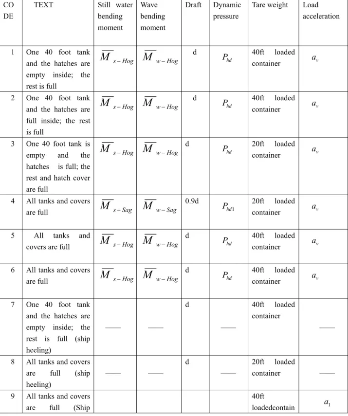
3.2.2 Load conditions required by the code

It shall be checked according to the calculation conditions in table 3.2(1). If there are more serious loading conditions other than table 3.2(1) in the loading manual, the structural strength of these loading conditions shall also be calculated directly. Figure 3.2(3) is the schematic diagram of each calculation condition.

Table 3.2(1) Load conditions CO

DE

TEXT Still water bending moment Wave bending moment Draft Dynamic pressure

Tare weight Load acceleration

1 One 40 foot tank and the hatches are empty inside; the rest is full

Hog s

M

M

2 One 40 foot tank and the hatches are full inside; the rest is full

Hog s

M

M

3 One 40 foot tank is empty and the hatches is full; the rest and hatch cover are full

Hog s

M

M

4 All tanks and covers

are full

M

M

1

hd

P 20ft loaded

container av 5 All tanks and

covers are full

M

M

hd

P 40ft loaded

container av 6 All tanks and covers

are full

M

M

hd

P 40ft loaded

container av 7 One 40 foot tank

and the hatches are empty inside; the rest is full (ship heeling) —— —— d —— 40ft loaded container ——

longitudinal motion) —— —— — —— er 1 0 Damaged (ship heeling) —— —— dam d —— 40ft loaded container —— Note: (1) d — draft, m;

(2) Heavy box — the allowable stack weight of a single box divided by the maximum number of packing layers

(3)Light box — the weight of a single box shall be no more than the following: In cargo hold: 55% of the weight of heavy container

On hatch cover: 90% of the allowable stack weight on hatch cover divided by the maximum number of packing layers or 17 tons, take the smaller one

(5) If a cargo hold contains two or more than 40 foot containers, each container must be calculated as empty

In the heeling condition (condition 7, condition 8), the load components are calculated by assuming the ship's static heeling to the maximum roll angle. The transverse load

component of the container in the cargo hold acts on the transverse bulkhead in the form of a set of concentrated forces according to the distribution position of the corresponding box angle in the transverse bulkhead. The transverse load component of the container on deck acts on the element node at the top of the transverse hatch coaming in the form of a set of shear forces distributed along the transverse direction.

If the container ship is equipped with a box type deck longitudinal truss and the span of the transverse torsional box of the deck is not more than 13.0m, it is unnecessary to calculate condition 9.

In surge condition (condition 9), the longitudinal force of each container in the cargo tank due to the longitudinal acceleration shall be transmitted to the main members of the transverse bulkhead (or transverse support bulkhead) from the corresponding angular position of the container according to the physical position of each container. The container load on the hatch cover shall be calculated as follows:

(1) The longitudinal force of the container on each hatch cover shall be determined according to the longitudinal acceleration at the high and middle points of the pile on the hatch cover, excluding the moment generated by the longitudinal force at the base of each pile.

(2) The stacking weight and number of layers of the container shall be taken according to the maximum stacking weight and number of layers allowed in the loading manual or cargo operation manual.

(3) The container load from the side of the deck to the coaming of the longitudinal hatch is not considered.

(4) 15% of the total longitudinal force on the hatch cover shall act on the nodes at the top of the longitudinal and transverse hatch coaming in the form of distributed force to simulate the friction force of the supporting block at the hatch coaming due to the longitudinal movement.

(5) The remaining 85% of the total longitudinal force on the hatch cover shall act on the node corresponding to the longitudinal stop slider at one end of the hatch cover (top of the transverse hatch coaming). If the position of the stop block is unknown, it is assumed to be 1 / 2 of the rear end width of the hatch cover. If the number of hatch covers is unknown, it is assumed that each hatch is covered by three hatch covers.

In the damaged condition (condition 10), it is assumed that any cargo tank of the ship enters the deepest balance water line. In the finite element model, only the damage of intermediate cargo tank and ballast tank on the same side is considered. The maximum height ddam2and the middle longitudinal section ddam at the same damage point are

3.3 Boundary conditions

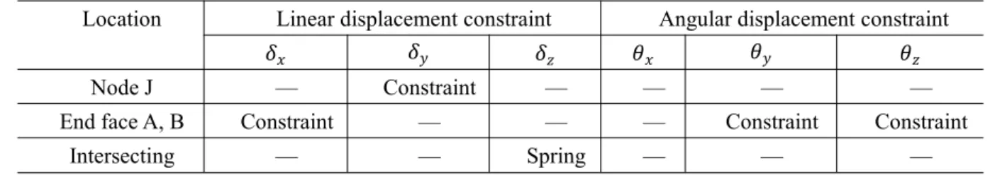
Table 3.3(1) is for the boundary conditions of load symmetrical calculation conditions (conditions 1, 2, 3, 4, 5, 6 and 9), table 3.3(2) is for the boundary conditions of load asymmetrical calculation conditions (conditions 7, 8 and 10), the node, intersection line and end surface in the table are shown in figure 3.3(1).

Figure3.3(1) Boundary conditions

For the calculation condition with symmetrical load, the vertical spring element shall be set at the joint of outboard plate, inner shell plate and front and rear transverse bulkheads. For the calculation condition with asymmetrical load, in addition to the vertical spring element on the intersection line of the side outer plate, inner shell plate and the front and rear transverse bulkheads, the horizontal spring element should also be set on the intersection line of the ship bottom plate, inner bottom plate and the front and rear transverse bulkheads. The elastic coefficient of spring element is uniformly distributed and calculated according to the following formula:

K = ᜰତ /

-G--- shear modulus of elasticity of material, for steel, G = .79 × /

A--- shear area of side shell plate, inner shell plate, bottom plate and inner bottom plate at front and rear bulkheads,

--- length of middle cargo tank, mm;

n---the number of vertical intersection nodes on the side outer plate and inner shell plate or the number of horizontal intersection nodes on the ship bottom plate and inner bottom plate.

Location Linear displacement constraint Angular displacement constraint

Node J — Constraint — — — —

End face A, B Constraint — — — Constraint Constraint

Intersecting — — Spring — — —

Table 3.3(2) Boundary condition of asymmetric load

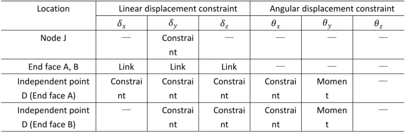
The boundary condition of the overall load case is shown in table 3.3(3), which is only applicable to the calculation of the bending stress of the hull girder. An independent point D is built at the intersection of the middle section and the axis and the longitudinal middle section in the end faces A and B (Fig. 3.3(1)). When the total longitudinal bending moment is applied on the independent point, the joint degrees of freedom of each longitudinal member at the end face are δx, δy, δz point correlation. The constraints of lateral linear displacement, vertical linear displacement and angular displacement around the

longitudinal axis of independent point D in end faces A and B are: = = = . Longitudinal line displacement constraint of independent point D in end face A is =

Table 3.3(3) Boundary condition of total load

3.4 Strength assessment

The plate element adopts the middle plane stress and the beam element adopts the axial stress. The stress of main components corresponding to standard working conditions shall not exceed the value given in table 3.4(1). For bulkheads, the stress at the end of the groove can be extrapolated from the average stress in the bulkhead plate. The average shear stress τ refers to the average shear stress within the web depth of the main member. The element

line EG,FH

Location Linear displacement constraint Angular displacement constraint End face A, B Constra

int — — — Constra int Constra int Intersecting line EG,FH — — Spring — — — Intersecting line IK,JL — Spring — — — —

Location Linear displacement constraint Angular displacement constraint Node J — Constrai

nt

— — — —

End face A, B Link Link Link — — — Independent point D (End face A) Constrai nt Constrai nt Constrai nt Constrai nt Momen t — Independent point D (End face B) — Constrai nt Constrai nt Constrai nt Momen t —

Component name Load condition Permissible stress(N/ mm2)

[σ_e] [τ] Deck plate LC1,2,3,4,5,6 225/K — Bottom plate LC1,2,3,4,5,6 225/K — Side plate, longitudinal bulkhead LC1,2,3,4,5,6 225/K 115/K Bottom girder LC1,2,3,4,5,6 235/K 115/K Double bottom floor LC1,2,3,4,5,6,7,8 175/K 90/K Horizontal strong frame LC1,2,3,4,5,6,7,8 195/K 95/K Side tank longitudinal platform LC1,2,3,4,5,6 225/K —

LC7,8 175/K 90/K

Transverse bulkhead plating LC1,2,3,4,5,6 180/K 100/K

LC10 235/K —

Transverse bulkhead girder LC1,2,3,4,5,6,7,8 175/K —

LC9 85/K —

LC10 235/K —

Connection between double bottom and side platform and watertight transverse bulkhead

LC10 235/K —

Transverse torsional box of deck LC7,8 175/K 90/K

LC9 85/K —

L10 235/K —

Toe end of bracket plate LC1,2,3,4,5,6,7,8,9,10 220/K —

Note:

In load condition 9, the element located at the joint of the hatch cover support block at the top of the hatch coaming. Since the joint supports the load directly from the hatch cover, the allowable value of the equivalent stress is[σ_e]95/K _{N/ mm}2

3.5 Summary of this chapter

This chapter gives a detailed introduction and analysis of the classification code for steel sea going ships in other aspects such as the finite element model, boundary condition definition, design load type and calculation method, structural evaluation criteria, which also paves the way for the direct calculation and analysis of the yield strength of the ship in Chapter 4.

4. Direct calculation and analysis of yield

strength of real ship

In this part, the finite element model of 24000DWT multifunctional container ship built by a shipyard in Shanghai is analyzed. The 24000DWT multi-purpose container ship has the typical structural arrangement characteristics of container ships, so it is selected as the target ship of ship structural safety assessment. According to the specification issued by CCS and reducing the calculation resources, the 1 / 2 + 1 / 2 cabin of the target ship is modeled and analyzed, the strength of all structures in the middle cabin of the model is evaluated, and the structural safety of the ship is analyzed.

According to relevant statistics, the failure of hull girder is usually due to the buckling and plastic deformation of stiffeners of deck, bottom or sometimes side shell plate. The failure of stiffeners in deck, bottom or side shell will lead to further damage and eventually the complete failure of hull girder. Therefore, in the study of the safety of ships, it is particularly important to focus on the structural safety of ships. In this chapter, the safety calculation of ship structure will be carried out from five aspects: basic information of calculation model, structure grouping of model, loading mode, calculation condition and load application.

4.1 Basic information of real ship model

(1) Main dimension of real ship

Table 4.1(1) Main dimension of real ship

(2) Model range

The selection of the finite element model of the container ship's hold section is generally within the range of the hold (1 / 2 + 1 + 1 / 2). Since the structure of the parallel middle body and the application of load do not change, the model is simplified to the range of (1 / 2 + 1 / 2).

Longitudinal direction: from stern to bow in x-axis. The range is fr85 ~ fr135.

Transverse direction: from starboard to port with y-axis. The model is symmetrical along the center line, and the half width of the model is 12.35m.

Vertical direction: from the bottom outer plate to the superstructure with Z axis.

Loa Lwl Lpp Breadth Depth Designed Draft

DWT Cargo capacity 160.31m 153.80m 149.60m 24.70m 13.50m 9.65m 24000t 29541.81m³

finite element mesh and additional properties are divided. b. Determine the boundary conditions of the model.

c. According to CCS specification, determine the calculation conditions required to be evaluated.

d. According to CCS specification, apply the cargo pressure inside the cabin, the water pressure outside the ship and the end bending moment.

e. Determine the allowable stress standard of different materials. f. Calculate the yield strength of the structure and analyze the results. (4) Material:

The whole model structure is composed of low carbon steel with the following steel properties:

Modulus of elasticity E=2.1E05 N/mm Poisson's ratio μ = 0.274

Material density ρ=7.83e-9 ton/mm

In this paper, the Gauss point stress value of each element is used to analyze the stress results. We define the result of stress at any point as (σ x, σ y, τ), which is calculated by the following formula:

σE = σx σy σx·σy τ

4-The model thickness is shown in Figure 4.1(1)

Figure4.1(1) Model of thickness

(5)Calculation parameters

According to the loading manual and other data of the target ship, the bending moment of the target ship in various states is shown in Schedule 1.

The permission design bending moment between Fr85 and Fr135 and the permission static bending moment in the port state are shown in table 4.1(1).

Table4.1(1) Permission bending moment

The beam element is used to select the light weight aggregate. The panel and web of the composite section bar (T profile) can be used as the rod unit, and the plate can be selected as the plate unit. The spacing of the ribs or the spacing of each longitudinal bone in the longitudinal direction shall be one unit, and at least three units shall be divided in the web height direction of the main supporting members. It can be used to delete the corresponding elements to simulate the web of the strong frame and the opening of the solid rib plate in the double bottom area, at the same time, it can also be used to reduce the thickness of the plate.

Figure4.1.2 FEM model of 1/2+1/2 cargoes Figure4.1.3 FEM half model of 1/2+1/2 cargoes Position DesignMs(+) (kN·m) DesignMs(-) (kN·m) HarbourMs(+) (kN·m) HarbourMs(-) (kN·m) Fr71 716000 -573680 1024007 -900433 Fr91 716000 -573680 1087241 -967516 Fr105+605 716000 -573680 1087241 -967516 Fr110 716000 -573680 1087241 -967516 Fr130 716000 -573680 1087241 -967515 Fr148 716000 -573680 1030511 -907332

4.2 Boundary conditions and Model grouping

4.2.1 Boundary conditions

It is assumed that the back face of the model is flat, and an independent point is established at the middle axis of the section. Other nodes on the end face are related to the independent point, and the moment is applied at the independent point.

It is assumed that the front end face of the model is flat, and an independent point is established at the neutral axis of the section. Other nodes on the end face are related to the independent point, and the bending moment is applied at the independent point.

Table 4.2(1) shows the detail of boundary conditions.

Table 4.2(1) Boundary condition of symmetrical load

Table 4.2(2) Boundary condition of total load

4.2.2 Model grouping

The purpose of model grouping is to manage and analyze models better and more efficiently. The model group of the target ship can be divided into two categories: one is the model group for model management, and the other is the structural model classification for bone profile. The former group is the ships according to the spatial position of the structure, such as vertical and horizontal, and names the actual structure name. The latter is the grouping of material name, size and structure. The model management groups are shown in the table 4.2(3).

Location Linear displacement constraint Angular displacement constraint

Node J — Constraint — — — —

End face A, B Constraint — — — Constraint Constraint Intersecting line

EG,FH

— — Spring — — —

Location Linear displacement constraint Angular displacement constraint

Node J — Constraint — — — —

End face A, B Link Link Link — — — Independent point

D (End face A)

Constraint Constraint Constraint Constraint Moment — Independent point

D (End face B)

Table 4.2(3) Typical structure management group of model

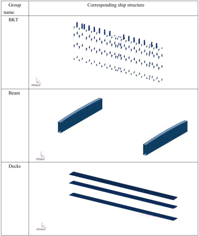
Group name

Corresponding ship structure BKT

Beam

Frame

InBottom

InShell

Plates grouping is shown in the figure 4.2(1).

Figure4.2(1) plates grouping

Outshell

4.3 Calculation condition and Loading mode

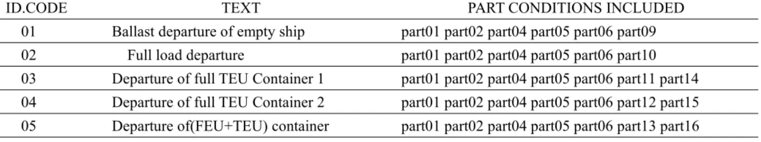
4.3.1 Typical calculation condition

According to CCS code, 5 typical working conditions are selected for calculation: (1)Ballast departure of empty ship

(2)Full load departure

(3)Full of container 1(Average weight 15t/TEU) departure(15t/869TEU,2.5t/528TEU) (4)Full of container 2(TEU)departure(24t/656TEU,14t/183TEU,2.5t/558TEU)

(5)Full of container 3(TEU+FEU)

departure(24t/176TEU,14t/35TEU,2.5t/52TEU,30.48t/240FEU,20t/139FEU,3.85t/188FEU) As shown in the table4.3(1)

Table 4.3(1) Load condition and part conditions included

The details of the part 01 to part 16 is shown in the appendix.

4.3.2 Loading mode

Loading mode is the way of loading cargo and ballast water. According to the different types of ships, the loading mode is mainly divided into bulk carrier loading mode and oil tanker loading mode. This ship is a multifunctional container ship, which can carry bulk cargo and containers. The different loading modes of the middle cabin are evaluated and analyzed. As shown in the table4.3(2).

Table4.3(2) 24000DWT multifunctional container ship cargo area loading mode

Loading ID.CODE

TEXT Loading Mode Loading

ID.CODE TEXT PART CONDITIONS INCLUDED 01 Ballast departure of empty ship part01 part02 part04 part05 part06 part09 02 Full load departure part01 part02 part04 part05 part06 part10 03 Departure of full TEU Container 1 part01 part02 part04 part05 part06 part11 part14 04 Departure of full TEU Container 2 part01 part02 part04 part05 part06 part12 part15 05 Departure of(FEU+TEU) container part01 part02 part04 part05 part06 part13 part16

01 Ballast departure of empty ship

02 Full load departure

03 Departure of full TEU Container 1

04 Departure of full TEU Container 2

05 Departure of(FEU+TEU) container

Where，BBWT is the Ballast of bottom tank, SBWT is the Ballast of side tank,

CH2 is the NO.2 Cargo hold and hatch coaming, CH3 is the NO.3 Cargo hold and hatch coaming, CONH2 is the NO.2 Container and hatch coaming, CONH3 is the NO.3 Container and hatch coaming.

4.4 Load application

Through the discussion of the chapter3.2, it can be known that the design load required to be calculated in CCS specification includes cargo pressure, water pressure outside the ship and end bending moment. It can be calculated by the formula and applied to the finite element model for structural strength analysis. The design load can be added manually in patran as follows:

(1) Grouping ， separate the same kind of components into cargo compartments, and adjust the normal direction of the elements to make the normal direction of each component consistent, so as easy to load.

(2) According to various loading conditions and stability calculations, the cargo pressure in the cabin can be calculated according to the proportion of cargo in the cabin.

w l g CH CH w l g CH CH / ) 8 / 5 ( ) 10 ( 3 ) 10 ( 3 / ) 2 / 1 ( ) 10 ( 2 ) 10 ( 2       l w g CONH CONH l w g CONH CONH         ) 8 / 5 ( ) 11 ( 3 ) 11 ( 3 ) 2 / 1 ( ) 11 ( 2 ) 11 ( 2 l w g CONH CONH l w g CONH CONH         ) 8 / 5 ( ) 12 ( 3 ) 12 ( 3 ) 2 / 1 ( ) 12 ( 2 ) 12 ( 2 l w g CONH CONH l w g CONH CONH         ) 8 / 5 ( ) 13 ( 3 ) 13 ( 3 ) 2 / 1 ( ) 13 ( 2 ) 13 ( 2

The cargo space accounted for half of the second cargo space from rib 85, and the cargo space accounted for 5 / 8 of the third cargo space to rib 135. The cargo weight values of parts 10, 11 and 12 can be found in the appendix.

The function of ballast water is added as follows

(3) Outboard water pressure. By substituting the parameters of the ship into the formula, the overboard water pressure can be obtained.

g(d-z) ρ

P sw

Add the following field function

(4) Applied end bending moment

According to the loading manual of the ship, the end bending moment at the boundary of the finite element model of the working condition is 716000 (n * mm), details are shown in the appendix.

The application results of each load are shown in the table 4.4(1).

Table 4.4(1) Load application under various calculation condition

4.5 Calculation and analysis

This section will mainly analyze the stress level of each structure under the above five calculation conditions, and evaluate the safety of the selected structure and the structural stress level of the selected cabin. The stress analysis of each component under different working conditions is as follows:

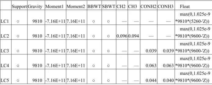
BBWT max(0,1.025e-9*9810*(1350-'Z)) SBWT max(0,1.025e-9*9810*(10600-'Z))

LC1 max(0,1.025e-9*9810*(5260-'Z)) LC2,3,4,5 max(0,1.025e-9*9810*(9600-'Z))

Support Gravity Moment1 Moment2 BBWT SBWT CH2 CH3 CONH2 CONH3 Float LC1 ○ 9810 -7.16E+11 7.16E+11 ○ ○ — — — — max(0,1.025e-9 *9810*(5260-'Z)) LC2 ○ 9810 -7.16E+11 7.16E+11 ○ ○ 0.096 0.094 — — max(0,1.025e-9 *9810*(9600-'Z)) LC3 ○ 9810 -7.16E+11 7.16E+11 ○ ○ — — 0.039 0.039 max(0,1.025e-9 *9810*(9600-'Z)) LC4 ○ 9810 -7.16E+11 7.16E+11 ○ ○ — — 0.063 0.063 max(0,1.025e-9 *9810*(9600-'Z)) LC5 ○ 9810 -7.16E+11 7.16E+11 ○ ○ — — 0.044 0.040 max(0,1.025e-9 *9810*(9600-'Z))

(1) Decks

Table4.5(1) Deck max and min stress

It can be seen from the table 4.5(1) that the deck meets the yield strength under all working conditions, and the ratio of the maximum stress to the allowable force is 0.684 251 . 1 / 225

123 _{ , indicating that the material has a large margin.}

(2) Frames

Table4.5(2) Frame max and min stress

It can be seen from the table 4.5(2) that the frame meets the yield strength under all working conditions, and the ratio of the maximum stress to the allowable force is 0.712 251 . 1 / 195

111 _{ , indicating that the material has a margin.}

ID.Code Von Miss(N/mm @Nd LC1 MAX 1.14E+02 5383 MIN 1.17E+01 14496 LC2 MAX 1.05E+02 757 MIN 6.25E+00 2504 LC3 MAX 1.23E+02 5383 MIN 5.65E+00 14491 LC4 MAX 1.13E+02 5383 MIN 5.22E+00 14491 LC5 MAX 1.22E+02 5383 MIN 5.55E+00 14491

ID.Code Von Miss(N/mm @Nd LC1 MAX 1.03E+02 14476 MIN 4.45E+00 17966 LC2 MAX 9.91E+01 9758 MIN 2.93E+00 9417 LC3 MAX 1.11E+02 14476 MIN 4.29E+00 16819 LC4 MAX 1.02E+02 14476 MIN 4.92E+00 7402 LC5 MAX 1.10E+02 14476

MIN 5.18E+00 16819 Figure4.5(2)Frame maximum stress nephogram Figure4.5(1)Deck maximum stress nephogram