LOCAL SOLUTIONS WITH POLYNOMIAL DECAY IN THE VELOCITY VARIABLES TO THE BOLTZMANN EQUATION FOR SOFT POTENTIALS (Mathematical Analysis in Fluid and Gas Dynamics)

(1)

LOCAL

SOLUTIONS

WITH POLYNOMIAL DECAY IN THE

VELOCITY

VARIABLES

TO THE BOLTZMANN EQUATION

FOR SOFT POTENTIALS YOSHINORI MORIMOTO AND TONG YANG

GRAD. SCHOOL OFHUMAN&ENVIRON.STUDIES, DEP. OF MATHEMATICS,

KYOTO UNIVERSITY, CITY UNIVERSITY OF HONG KONG

1. INTRODUCTION

In the present note

we

consider the Cauchy problem for the spatially inhomoge-neous Boltzmann equation,

(1.1) $\partial_{t}f+v\cdot\nabla_{x}f=Q(f, f) , f(O,x,v)=f_{0}(x, v)$,

where $f=f(t, x, v)$ is the density distribution function of particles with velocity

$v\in \mathbb{R}^{3}$ at time $t$ and position $x$

.

The right hand side of (1.1) is given by the

Boltzmann bilinear collision operator

$Q(g, f)(v)= \int_{\mathbb{R}^{3}}\int_{\mathbb{S}^{2}}B(v-v_{*}, \sigma)\{g(v_{*}’)f(v’)-g(v_{*})f(v)\}d\sigma dv_{*},$

where the conservation of momentum and energy implies that for $\sigma\in \mathbb{S}^{2}$

$v’= \frac{v+v_{*}}{2}+\frac{|v-v_{*}|}{2}\sigma, v_{*}’=\frac{v+v_{*}}{2}-\frac{|v-v_{*}|}{2}\sigma.$

The non-negative

cross

section $B$ usually takes the form

(1.2) $B= \Phi(|v-v_{*}|)b(\cos\theta) , \cos\theta=\frac{v-v_{*}}{|v-v_{*}|} \sigma, 0\leq\theta\leq\frac{\pi}{2},$

where

$\Phi(|z|)=\Phi_{\gamma}(|z|)=|z|^{\gamma}$, for

some

$\gamma>-3,$

$b(\cos\theta)\theta^{2+2s}arrow K$ when $\thetaarrow 0+$,for $0<s<1$ and $K>0.$

In fact, for the physical model, if the inter-molecule potential satisfies the inverse

power law potential $U(\rho)=\rho^{-(q-1)},$_$q>2($, where $\rho$ denotes the distance between

twointeracting molecules), then $s$ and $\gamma$

are

given by

$0<s=1/(q-1)<1, 1>\gamma=1-4_{\mathcal{S}}=(q-5)/(q-1)>-3.$

As usual, the hard $(\gamma>0)$ and soft $(\gamma<0)$ potentials correspond to $q>5$ and

$2<q<5$, respectively, and the Maxwelhan potential $(\gamma=0)$ corresponds to $q=5.$

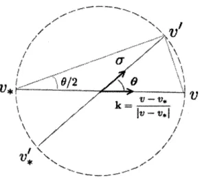
The angle$\theta$isthe deviationangle, i.e., the angle between post- and pre-collisional

velocities (see Figure 1 in the next page). Though the range of $\theta$ is originally a

full interval $[0, \pi]$, it should be noted that the angle $\theta$ in (1.2) is now restricted to

$[0, \pi/2]$, as in [1], by replacing $b(\cos\theta)$ by its ’symmetrized” version $[b(\cos\theta)+b(\cos(\pi-\theta))]1_{0\leq\theta\leq\pi/2},$

(2)

FIGURE 1. post- and pre-collisional velocities

which is possible due to the invariance of the product $f(v’)f(v_{*}’)$ in the collision

operator $Q(f, f)$ _{under the change of variables} $\sigmaarrow-\sigma$

.

This device enables us to

use the regularchange ofvariables between post- and pre-collisional velocities (in

the proof of the celebrated cancellation lemma in [1]$)$,

$v \mapsto v’=\frac{v+v}{2}*+\frac{|v-v_{*}|}{2}\sigma,$

where the Jacobian is found to be

$| \frac{\partial v}{\partial v’}|=\frac{8}{|I+k\otimes\sigma|}=\frac{8}{|1+k\cdot\sigma|}=\frac{4}{\cos^{2}(\theta/2)}\leq 8, \theta\in[0, \pi/2].$

In [15, 2], the singularchange of variables$v_{*}arrow v’$ (, whose Jacobianis computed

as

$| \frac{\partial v_{*}}{\partial v’}|=\frac{8}{|I-k\otimes\sigma|}=\frac{8}{|1-k\cdot\sigma|}=\frac{4}{\sin^{2}(\theta/2)}\sim\theta^{-2}, \theta\in[0, \pi/2],)$

was also introduced to show the existence of solutions to the‘linearized”

Boltz-mann equation, and was used in [3, 4, 9] to prove the uniqueness ofsolutions with

polynomial decay in the velocity variable to the nonlinear Boltzmann equation for Maxwellian and soft potentials. Especially in [9], the uniqueness of solutions was considered in the following function space; for $m\in \mathbb{R},$$\ell\geq 0$ and $T>0,$

$\mathcal{P}_{\ell}^{m}([0, T]\cross \mathbb{R}_{x,v}^{6}) = \{f\in C^{0}([0, T];S’(\mathbb{R}_{x,v}^{6}))$;

$s.t. f\in L^{\infty}([0, T]\cross \mathbb{R}_{x}^{3};H_{\ell}^{m}(\mathbb{R}_{v}^{3}))\},$

$\Vert f\Vert_{H_{\ell}^{m}(\mathbb{R}_{v}^{3})}=(\int_{\mathbb{R}^{3}}|\langlev\rangle^{\ell}(\langle D_{v}\rangle^{m}f(v))|^{2}dv)^{1/2} \langle v\rangle=(1+|v|^{2})^{1/2}$

An effective use ofthe singularchange ofvariables gives us

Theorem 1.1 ([9]). Assume that the cross section $B$ takes the

form

(1.2) with

$0<s<1$

and $\max\{-3, -3/2-2s\}<\gamma\leq 0$

.

Suppose that the Cauchy problem (1.1) admits two weak solutions $f_{1}(t),$$f_{2}(t)\in \mathcal{P}_{\ell_{0}}^{2s}([0, T]\cross \mathbb{R}_{x,v}^{6})$ with $0<T<+\infty$

and$\ell_{0}\geq 14$ having the

same

initial datum

$f_{0}\in L^{\infty}(\mathbb{R}_{x}^{3};H_{\ell 0}^{2s}(\mathbb{R}_{v}^{3}))$

.

If

one solution

(3)

Here the weak solution to the Cauchy problem (1.1) is defined by

$\int_{\mathbb{R}^{6}}f(t, x, v)\eta(t, x, v)dxdv-\int_{\mathbb{R}^{6}}f_{0}(x,v)\eta(0, x, v)dxdv$

$- \int_{0}^{t}d\tau\int_{\mathbb{R}^{6}}f(\tau, x, v)(\partial_{\tau}+v\cdot\nabla_{x})\eta(\mathcal{T}, x, v)dxdv$

$= \int_{0}^{t}d\tau\int_{\mathbb{R}^{6}}Q(f, f)(\tau,x, v)\eta(\tau, x, v)dxdv,$

where $\eta\in C^{1}(\mathbb{R};C_{0}^{\infty}(\mathbb{R}^{6}))$ is a test function.

Comparedwith theuniquenessof polynomial decay solutions in the velocity vari-ables, there are few results concerning the existence of such slowly decay solutions

in spatially inhomogeneous case (cf., renormalized solutions by [13, 11], and [12] in

the cutoff case). In fact, the existence of classical solutions for the spatially

inho-mogeneous Boltzmann equation has been usually discussed for solutions with the Maxwellian decay weight in the velocity variables (see [3, 4, 5, 6, 8, 10, 14] in the non-cutoff case). In the next section we state a local existence result concerning polynomial decay solutions in the velocity variable to the full nonlinear Boltzmann

equation in a certain soft potential case, by aneffective

use

of the singular change

ofvariables between post- and pre-colhsional velocities.

2. LOCAL EXISTENCE FOR SOFT POTENTIALS Throughout this sectionwe confine ourselves to the

case

(2.3) $0<s< \frac{1}{2}, -\frac{3}{2}<\gamma\leq 0,$

because of the technical difficulties, though the uniqueness result,Theorem 1.1,

holds under the

more

general situation$0<s<1$ and$\max\{-3, -2_{\mathcal{S}}-3/2\}<\gamma\leq 0.$

We introduce our working function spaces as follows: Set

$\partial_{\beta}^{\alpha}=\partial_{x}^{\alpha}\partial_{v}^{\beta}, \alpha, \beta\in \mathbb{N}^{3}.$

and

(2.4) $\mathcal{W}=\{\begin{array}{ll}\langle v\rangle if 0<s\leq 1/4,\langle v\rangle^{2s/(1-2s)} if 1/4<s<1/2,\end{array}$

which ensures $\langle v\rangle^{2s}\leq \mathcal{W}^{1-2s}$ and $\langle v\rangle\leq \mathcal{W}$ for the later use. As in [4, 7], we use a

kind ofcutoff function in both space and velocity variables,

(2.5) $\phi(x, v)=\frac{1}{1+|v|^{2}+|x|^{2}},$

which possesses the commutator property $|[v\cdot\nabla_{x},$$\phi||=2|v\cdot x|\phi^{2}\leq\phi$

.

For $k\in \mathbb{N},$ $\ell\in \mathbb{R}$with $k<\ell$, we define

(2.6) $\mathcal{H}_{u}^{k}|^{\ell}(\mathbb{R}^{6})=\{g|\Vert g\Vert_{\mathcal{H}_{u}^{k}}^{2}i^{\ell_{(\mathbb{R}^{6})}}$

$= \sum_{|\alpha+\beta|\leq k}\sup_{a\in \mathbb{R}^{3}}\int_{\mathbb{R}^{6}}|\phi(x-a, v)\mathcal{W}^{\ell-|\alpha+\beta|}\partial_{\beta}^{\alpha}g(x, v)|^{2}dxdv<+\infty\}.$

The function space $\mathcal{H}_{u}^{k}|^{\ell}(\mathbb{R}^{6})$ is a variant of the uniformly local Sobolev space

(4)

and a usual smooth cutoff function $\phi_{1}(x)\in C_{0}^{\infty}(\mathbb{R}^{3})$, respectively. In [8],

bounded classical solutions for the initial data $f_{0}(x, v)$ satisfying

(2.7) $\exists\rho_{0}>0s.t. e^{\rho_{0}\langle v\rangle^{2}}f_{0}\in H_{u}^{k}i^{0}(\mathbb{R}^{6})$

are constructed in _{the whole space without specifying any limit behaviors} _at _the

spatial infinity and without the smallness condition on initial data, under the

as-sumptions on the

cross

section $B$ with

$0<s<1/2, -3/2<\gamma, \gamma+2s<1.$

From the point view ofthe local existence of polynomial decay solution in the velocity variable, we have the following improvement ofTheorem 1.1 of [8] for the

soft potential case;

Theorem 2.1. Assume that the cross section $B$ takes the

form

(1.2) with (2.3),

that is, _$0<s<1/2,$ $-3/2<\gamma\leq 0$

.

If

the _initial _data $f_{0}$ is

non-ne9ative

and

belongs to $\mathcal{H}_{u}^{k}|^{\ell}(\mathbb{R}^{6})$

for

$k\geq 6,\ell\geq k+7$, then, there _exists a $T_{*}>0$ such that the

Cauchy problem (1.1) admits a non-negative unique solution in the

_function

space

$C^{0}([0, T_{*}];\mathcal{H}_{u}^{k}|^{\ell}(\mathbb{R}^{6}))$

.

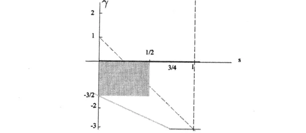
Remark 2.2. The rectangle below expresses the domain

_of

$(\gamma, s)$ covered by

Theo-rem

2.1. The previous _{local existence result} _{under (2.7) in [8]} _{covers an additional}

triangle region below the line $\gamma=1-2s$, which is _{contained in the} _hard _potential

region $\gamma>0$

.

Time global solutions near a global equilibrium,

$f=\mu+\sqrt{\mu}g, \mu=e^{-|v|^{2}/2}/(2\pi)^{3/2}.$

were given in [4, 5, 6], [14], which cover the

_full

region

$0<s<1$

, $\gamma>$

$\max\{-3, -3/2-2s\}$ _indicated _{by the figure below.}

$

FIGURE 2. dashed line: $\gamma=1-4s$ in case ofinverse power law _potential

For theproofof Theorem 2.1, weconstruct the approximatesolutions by angular cutoff approximation. That is, for $0<\epsilon\ll 1$, we approximate (cutoff) the cross

section by

(5)

Theorem 2.3 (Cutoff case). Assume that $-3/2<\gamma\leq 0$ and replace the angular

factor of

the

cross

section $b$ by$b_{\epsilon}$

.

If

the initial data $f_{0}$ is non-negative and belongs

to $\mathcal{H}_{u}^{k}|^{\ell}(\mathbb{R}^{6})$

for

_{$k\geq 5,$}$\ell\geq k+7$, then, there exists a $T_{\epsilon}>0$ such that the Cauchy

problem (1.1) admits a non-negative unique solution$f^{\epsilon}(t, x, v)$ in the

function

space

$C^{0}([0, T_{\epsilon}];\mathcal{H}_{u}^{k}|^{\ell}(\mathbb{R}^{6}))$

.

Remark 2.4. In the

_cutoff

case.

the order

_of

derivative $k$ can be taken not less

than 5 instead

_of

6

_for

the

_non-cutoff

case

in

our

analysis. We might improve the

$\partial_{x},\partial_{v}$

order.

$of$ derivatives by

use

of

the

fractional

derivatives employed in [10],

instead

of

Another key ingredient is to obtaina uniform estimate for solutions in the given function space. Let $T>0$ and $f(t)\in C^{0}([0, T];\mathcal{H}_{u}^{k}|^{\ell}(\mathbb{R}^{6}))$ with$k\geq 6$ and $\ell\geq k+7.$

If

we

put

$\mathcal{E}(t)=\Vert f(t)\Vert_{\mathcal{H}_{u}^{k}}^{2}i^{\ell}$_’

then there exists a $C>0$ depending only on $s,$$\gamma,$ $k,$$P$ and $K>0$ in the hypothesis

of$b$ such that

(2.8) $\mathcal{E}(t)\leq \mathcal{E}(0)+C\int_{0}^{t}\mathcal{E}(\tau)(1+\mathcal{E}(\tau))d\tau, t\in[0, T],$

wherewe refer [16] to thedetailderivation ofthis estimate, by

means

of both regular and singular changes of variables between post- and pre-collisional velocities. It follows from (2.8) that we have

$\mathcal{E}(t)\leq\frac{\mathcal{E}(0)e^{Ct}}{1-(e^{Ct}-1)\mathcal{E}(0)},$

by exactlythe

same

calculation

as

the

one

after (4.3.11) of [3]. If

we

choose $T_{*}>0$

small enough such that

$T_{*}= \frac{1}{C}\log(1+\frac{3}{1+4\Vert f_{0}\Vert_{\mathcal{H}_{u}^{k}}i^{\ell_{(\mathbb{R}^{6})}}})$

then we obtain a uniform estimate

(2.9) $\Vert f(t)\Vert_{\mathcal{H}_{u}^{k}}i^{\ell_{(\mathbb{R}^{6})}}\leq 2\Vert f_{0}\Vert_{\mathcal{H}_{u}^{k}}i^{\ell_{(\mathbb{R}^{6})}}$ for $t\in[O, T_{*}].$

The proofofTheorem 2.1 canbecompleted in the almost same way asinthe proof

of Theorem4.11 of [3] and the subsequent paragraph there, takinginto account the

uniform estimate (2.9) and Theorem 2.3.

REFERENCES

[1] R. Alexandre, L. Desvillettes, C. Villani and B. Wennberg, Entropy dissipation and

long-range interactions, Arch. Ration. Mech. Anal. 152 (2000), 327-355

[2] R.Alexandre, Y.Morimoto, S.Ukai, C.-J.Xu and T.Yang, Uncertainty principle and kinetic

equations, J. Funct. Anal., 255 (2008) 2013-2066.

[3] R. Alexandre, Y. Morimoto, S. Ukai, C.-J. Xu and T. Yang, Regularizing _effect and local

existence_for_non-cutoffBoltzmann equation, Arch. Ration. Mech. Anal.,198 (2010), 39-123.

[4] R. Alexandre, Y. Morimoto, S. Ukai,C.-J. Xuand T. Yang, Global existence and_full

regular-ity_ofthe Boltzmann equationwithout angular cutoff, Comm. Math. Phys.,$3-4-2(2011),513-$

581.

[5] R. Alexandre, Y. Morimoto, S. Ukai,C.-J. Xu and T. Yang, The Boltzmann equation without

angular _cutoffin the whole space: I. Global existence_{for soft} potential, J. Funct. Anal. 262

(6)

[6] R. Alexandre, Y. Morimoto, S. Ukai, C.-J. Xu, T. Yang, The Boltzmann equation without angular_cutoffin the whole space: $\Pi$, global existenceforhard potential, Anal. Appl. 9 (2011) 113-134,

[7] R. Alexandre, Y. Morimoto, S. Ukai, C.-J. Xu and T.Yang, Boltzmann equation without angular _cutoffin the whole space: Qualitative properties _ofsolutions, Arch. Rational Mech. Anal.,202(2011), 599-661.

[8] R. Alexandre, Y. Morimoto, S. Ukai, C.-J.Xu and T. Yang, Bounded solutions _ofthe

Boltz-mann equationin the whole space, Kinetic andRelated Models. 4 (2011) 17-40.

[9] R. Alexandre, Y. Morimoto, S. Ukai, C.-J. Xu and T. Yang, Uniqueness _of solution_for the non _cutoffBoltzmann Equation with the _soft potential, Kinet. Relat. Models, 4 (2011),

919-934.

[10] R. Alexandre, Y. Morimoto, S. Ukai, C.-J. Xu and T. Yang, Local existence with mild

regu-laroty_forthe Boltzmann equation, to appearin Kinet. Relat. Models, 4 (2013).

[11] R. Alexandre and C. Villani, On the Boltzmann equation_forlong-range interaction, Comm. Pure Appl. Math., 55 (2002), 30-70.

[12] L. Arkeryd, R. Esposito, M.Pulvirenti,. The Boltzmann equation_for weakly inhomogeneous data. Comm. Math. Phys. 111 (1987), 393-407.

[13] R. J. DiPerna and P. L. Lions, On the Cauchy problem _for Boltzmann equations: global existence and weak stability. Ann. Math., 130 (1989), 321-366.

[14] P.-T.Gressman and R.-M. Strain, Global classicalsolutions oftheBoltzmann equation

with-out angular _cut-off. J. Amer. Math. Soc., 24 (2011), 771-847.

[15] Y. Morimoto, S. Ukai, C.-J. Xu and T. Yang, Regularity _ofsolutions to the spatially

ho-mogeneous Boltzmann equation without angular cutoff, Discrete and Continuous Dynamical

Systems-Series A 24, (2009), 187-212.

[16] Y. Morimotoand T. Yang, Local existence _ofpolynomial decay solutions to the Boltzmann

equation_{for soft}potentials, to appearinAnal. Appl.

YOSHINORI MORIMOTO, GRADUATE SCHOOL OF HUMAN AND ENVIRONMENTAL STUDIES,

KYOTO UNIVERSITY, KYOTO, 606-8501, JAPAN

$E$-mail address: [email protected]

TONG YANG, DEPARTMENT OF MATHEMATlCS, CITY UNIVERSITY OF HONG KONG, HONG KONG, P. R. CHINA