A residual bound evaluation of operator equations with Raviart-Thomas finite element (The latest developments in theory and application on scientific computation)

(1)

A residual bound evaluation of operator equations with

Raviart-Thomas finite element

早稲田大学基幹理工学研究科高安亮紀 (Akitoshi Takayasu)1

Graduate SchoolofFundamental Science andEngineering,WasedaUniversity

早稲田大学劉雪峰 (Xuefeng Liu)2

FacultyofScienceand Engineering,Waseda University, CREST, JST

早稲田大学大石進一 (Shin’ichi Oishi)3

DepartmentofApplied Mathematics, FacultyofScience and Engineering,

Waseda

University,

CREST,

JST

Abstract –In this article, a residualevaluationof operator equation is considered in theframework

of computer-assisted proof. Our computer-assistedapproach

ensures

theexistence and local uniqueness of

weak solutions to

some

nonlinearpartial differentialequations. Based

on

Newton-Kantorovichtheorem,

our

numerical method is

a

variant of existing methods such

as

[1, 2, 3, 4]. Residual evaluation for operator equationplays important role in validatingnumerical solutions. In order to getaccurate residualevaluation,

some

smoothing techniqueshavebeenproposed. Mainobjective of thisarticle is toobtain

a

sharp bound

evaluationwith high order Raviart-Thomas mixed finite element.

1 Introduction

Let$\Omega$beboundedpolygonal domain in$\mathbb{R}^{2}$with arbitrary shape. $\mathbb{R}$isthe setofreal numbers. In this article,

we are

concerned with Dirichletboundaryvalueproblemof thesemi-linearelliptic equationofthe form:

$\{\begin{array}{ll}-\Delta u=f(\nabla u, u, x), in \Omega,u=0, on \partial\Omega\end{array}$ (1)

where $f$ : $H_{0}^{1}(\Omega)arrow L^{2}(\Omega)$ isassumed tobe Fr\’echet differentiable. For example, $f(\nabla u, u, x)=-b\cdot\nabla u-$ $cu+c_{2}u^{2}+c_{3}u^{3}+g$with$b(x)\in(L^{\infty}(\Omega))^{2},$$c,$$c_{2},$$c_{3}\in L^{\infty}(\Omega)$and$g\in L^{2}(\Omega)$satisfiesthis condition. Verified computation approach will be adopted to explore the existence and local uniqueness ofweak solution of

(1). Namely, if

an

approximate solution is given by certain numerical method,

we

willtry to validate the

existence ofexactsolution in the neighbourhood of theapproximation. Intheclassicalanalysisof variational

theory, weak solution of Dirichlet boundary problem (1) isdefined invariationalform:

Find$u\in H_{0}^{1}(\Omega)$, satisfying $(\nabla u, \nabla v)=(f(\nabla u, u, x), v)$, for all $v\in H_{0}^{1}(\Omega)$

.

(2)

Here,

$( \nabla u, \nabla v):=\int_{\Omega}\nabla u\cdot\nabla vdx$ and $(f( \nabla u, u,x), v):=\int_{\Omega}f(\nabla u, u, x)vdx$

.

Nowweput $V=H_{0}^{1}(\Omega)$and rewrite$f(\nabla u, u, x)$

as

$f(u)$ _for_simple_{form. Let}

us

_define_{linear and nonlinear}

operators$\mathcal{A},$ $\mathcal{N}:Varrow V$, $($Au,$v)_{V}$$:=(\nabla u, \nabla v),$$(\mathcal{N}(u), v)_{V}$ $:=(f(u), v)$

.

Furthermore,

we

define$\mathcal{F}:Varrow V$

as

$\mathcal{F}(u)$$:=\mathcal{A}u-\mathcal{N}(u)$

.

The original problem (1)isequivalent tothe followingnonlinearoperator equation:

Find $u\in V$, satisfying $\mathcal{F}(u)=0$

.

(3)

1_takitoshiQsuou._waseda.jp

$2_{xf1i}$_uQaoni._waseda._jp

(2)

$\mathcal{F}:Varrow V$ is assumed tobeFr\’echetdifferentiable mapping. Let $\hat{u}\in V_{h}\subset V$ be

an

approximate solution to

eq.(3). Fr\’echetderivativeof$\mathcal{F}$at$\hat{u}$ isdenotedby$\mathcal{F}’[\hat{u}]$:$Varrow V$

.

In ordertoverifythe existenceand local

uniqueness ofthe exact solution in the neighborhood of$\hat{u}$, we consider to apply the Newton-Kantorovich

theorem [5, 6] toeq.(3).

Theorem 1. AssumingFrechet derivative$\mathcal{F}’[\hat{u}]$ is nonsingular and

satisfies

$\Vert \mathcal{F}’[\hat{u}]^{-1}\mathcal{F}(\hat{u})\Vert_{V}\leq\alpha$,

for

a certain positive$\alpha$

.

Then, let$\overline{B}(\hat{u}, 2\alpha):=\{v\in V:\Vert v-\hat{u}\Vert_{V}\leq 2\alpha\}$ bea closed ball centered at$\hat{u}$ with radius $2\alpha$

.

Let also$D\supset\overline{B}(\hat{u}, 2\alpha)$ be

an

open ballin V. We

assume

that

for

a certain positive$\omega$, itholds:

$\Vert \mathcal{F}’[\hat{u}]^{-1}(\mathcal{F}’[v|-\mathcal{F}’[w|)\Vert_{V,V}\leq\omega\Vert v-w\Vert_{V},$ $\forall v,$$w\in D$

.

If

$\alpha\omega\leq\frac{1}{2}$ holds, then thereis

a

solution_{$u\in V$}

of

$eq.(3)$ satisfying

$\Vert u-\hat{u}\Vert_{V}\leq\rho:=\frac{1-\sqrt{1-2\alpha\omega}}{\omega}$

.

(4)

Furthermore, the solution$u$ is unique in$\overline{B}(\hat{u}, \rho)$

.

Remark 1. To apply Newon-Kantorovich theorem, we willcalculate the constants belowexplicitly.

$\Vert \mathcal{F}’[\hat{u}]^{-1}\Vert_{V,V}\leq C_{1}$, (5) $\Vert \mathcal{F}(\hat{u})\Vert_{V}\leq C_{2,h}$, (6)

$\Vert \mathcal{F}’[v]-\mathcal{F}’[w]\Vert_{V,V}\leq C_{3}\Vert v-w\Vert_{V}$, $\forall v,$$w\in D\subset V$

.

(7)

Therefore,

_if

$C_{1}^{2}C_{2},{}_{h}C_{3}\leq 1/2$ is

confirmed

by

verified

computations, thenthe existence and local uniqueness

of

the solution

are

proved numerically basedon Newton-Kantoromch theorem.

Themaintopic ofthis article is toevaluatethe residualbound for$\mathcal{F}(\hat{u}),$ $i.e$.

$\Vert \mathcal{F}(\hat{u})\Vert_{V}\leq C_{2,h}$

.

(8) In the following, we would like to introduce several ways to evaluateeq.(S). Supposefunction$\hat{u}\in V_{h}$ tobe

anapproximation ofexactsolutionofeq.(3), where$V_{h}$is certain finite elementsubspace$V_{h}\subset V$

.

Ouraim is

to obtain good estimation of this residual bound. First,weintroduce severalevaluation methods in Section

2. Second, we show numericalresults in Section3 to demonstrate the efficiency ofourproposed method. Forreader$s$convenience, wewrite downthe detailsfor implementationofRaviart-Thomaselementmethod

inappendix.

2 Several ways for residual evaluation

Inthissection, wewould like to consider the residual evaluation in the form of

$\Vert \mathcal{F}(\hat{u})\Vert_{V}=\sup_{0\neq v\in V}\frac{(\mathcal{A}\hat{u}-\mathcal{N}(\hat{u}),v)_{V}}{\Vert v||_{V}}=\sup_{0\neq v\in V}\frac{|(\nabla\hat{u},\nabla v)-(f(\hat{u}),v)|}{||v\Vert_{V}}$

inseveralways. If

an

approximate solutionsatisfies$\hat{u}\in H^{2}(\Omega)\cap V_{h}$,itfollows

$\Vert \mathcal{F}(\hat{u})\Vert_{V}=\sup_{0\neq v\in V}\frac{|(\nabla\hat{u},\nabla v)-(f(\hat{u}),v)|}{||v\Vert_{V}}=\sup_{0\neq v\in V}\frac{|(-\Delta\hat{u},v)-(f(\hat{u}),v)|}{||v\Vert_{V}}\leq C_{e,2}\Vert\triangle\hat{u}+f(\hat{u})\Vert_{L^{2}}$

.

(9)

Here, $C_{e,p}$

means

Sobolev$s$embedding constant, which satisfies $\Vert u\Vert_{L^{p}}\leq C_{e,p}|u|_{H^{1}},$ $(2\leq p<\infty)$ for$u\in V$.

We point out thatthe evaluation (9) doesnot work when $V_{h}$ is taken as $C^{0}$ finite element functions,such

as

$P_{1}$ (piecewise linear)or$P_{2}$ (piecewise quadratic) elements. This is because$\triangle\hat{u}$ doesnot belong to$L^{2}(\Omega)$

anymore.

Toweaken thecondition

on

$\hat{u}$, we will introduceseveralmethods that donot need the$H^{2}$-regularityof

approximate solution. Thefirst method tobe introducedisfast but giveslittle rough bound. The second

one

has accurate estimation withsmoothing technique. Thethird

one

isbased onRaviart-Thomas mixed

(3)

2.1 Simple

bounds

Let $V_{h}$ be

a

finite element subspace of$V$, such that $V_{\hslash};=$ span$\{\phi_{1}, \ldots, \phi_{n}\}$

.

Let $u_{h};=\prime P_{h}u\in V_{h}$ be

an

orthogonalprojectionof$u\in V$,defined

as

$(\nabla(u-u_{h}), \nabla v_{h})=0,$ $\forall v_{h}\in V_{h}$In this part,

we

will showsimple

upperbound of residue. Inthefollowing, we denote$v_{\hslash}$ by the projection of$v,$ $i.e$

.

$P_{h}v$

.

From the

classical

error

analysis, such

as

Aubin-Nitsche’strick,

we

have

$\Vert v-v_{h}\Vert_{L^{2}}\leq C_{M}\Vert v-v_{h}\Vert_{V}$, (10)

$\Vert v-v_{h}\Vert_{V}\leq\Vert v\Vert_{V}$ and $\Vert v_{h}$

llv

$\leq\Vert v\Vert_{V}$

.

(11)

Here$C_{M}$ isapriori

error

constantfor projection$\mathcal{P}_{h}$

.

The full discussion of this constant

on

arbitrarydomain is shown in [12]. For$v_{h}\in V_{h}$,the residualbound ofeq.(8) isgivenusing inequalities (10) and (11)

$\Vert \mathcal{F}(\hat{u})\Vert_{V}$ $=$ $\sup_{0\neq v\in V}\frac{|(\nabla\hat{u},\nabla v)-(f(\hat{u}),v)|}{\Vert v\Vert_{V}}$

$=$ $\sup_{0\neq v\in V}\frac{|(\nabla\hat{u},\nabla(v-v_{h}))-(f(\hat{u}),v-v_{h})+(\nabla\hat{u},\nabla v_{h})-(f(\hat{u}),v_{h})|}{\Vert v||_{V}}$

$\leq$ $\sup_{0\neq v\in V}\frac{|(f(\hat{u}),v-v_{h})|}{||v\Vert_{V}}+\sup_{0\neq v\in V}\frac{|(\nabla\hat{u},\nabla v_{h})-(f(\hat{u}),v_{h})|}{\Vert v\Vert_{V}}$

$\leq$ $C_{M}$

llf

$(\hat{u})\Vert_{L^{2}}+C_{r}$ (12)

wherethe quantity $C_{r}$ is definedbythefollowing procedure

$\sup_{0\neq v\in V}\frac{|(\nabla\hat{u},\nabla v_{h})-(f(\hat{u}),v_{h})|}{\Vert v\Vert_{V}}$ $=$ $0^{0\neq v\in V} \sup_{=v_{h}\in V_{h}}\frac{|(\nabla\hat{u},\nabla v_{h})-(f(\hat{u}),v_{\hslash})|}{||v\Vert_{V}}+0^{0\neq v\in V}\sup_{\neq v_{h}\in V_{h}}\frac{|(\nabla\hat{u},\nabla v_{h})-(f(\hat{u}),v_{h})|}{\Vert v_{h}||_{V}}\cdot\frac{\Vert v_{h}\Vert_{V}}{||v\Vert_{V}}$

$\leq$ $\sup_{0\neq v_{h}\in V_{h}}\frac{|(\nabla\hat{u},\nabla v_{h})-(f(\hat{u}),v_{h})|}{\Vert v_{h}\Vert_{V}}=:C_{r}$

.

Let$\epsilon_{i}$ be $\epsilon_{i}$ $:=(\nabla\hat{u}, \nabla\phi_{i})-(f(\hat{u}), \phi_{i}),$ $(i=1, \ldots, n)$

.

Since$v_{h}\in V_{h}$,

we

can

express $v_{h}$

as

$v_{h}$ $:= \sum_{i=1}^{n}c_{i}\phi_{i}$

.

Let

us

put $c:=(c_{1}, \ldots, c_{n})^{t}$ and$\epsilon;=(\epsilon_{1}, \ldots, \epsilon_{n})^{t}$

.

Let

further

$D$ be$n\cross n$matrixwhose $(i,j)$-elements

are

given by$(\nabla\phi_{i}, \nabla\phi_{j})$

.

Then,

C.

follows

$C_{r}= \sup_{0\neq v_{h}\in V_{h}}\frac{|(\nabla\hat{u},\nabla v_{h})-(f(\hat{u}),v_{h})|}{||v_{h}\Vert_{V}}=\sup_{c\in R^{n}}\frac{|\sum_{i=1}^{n}q\epsilon_{i}|}{\sqrt{c^{t}Dc}}\leq\sup_{c\in R^{n}}\frac{|c|_{l^{2}}|\epsilon|_{l^{2}}}{\sqrt{c^{t}Dc}}\leq\Vert D^{-1}\Vert_{2}|\epsilon|_{l^{2}}$

.

(13)

Frominequalities (12) and (13),

we

obtain

$\Vert \mathcal{F}(\hat{u})\Vert_{V}\leq C_{M}\Vert f(\hat{u})\Vert_{L^{2}}+\Vert D^{-1}\Vert_{2}|\epsilon|_{l^{2}}$

.

(14)

2.2 Accurate

bounds with

a

smoothing technique

The simple bound(14) isaroughbound. overestimation often

causes

failurein verification. Next, another

methodforevaluating the residual bound isintroduced. This isbased onthe smoothing technique proposed

by N. Yamamoto et. al. [13]. Here, smoothing

means

to approximate vector $\nabla\hat{u}$ by smooth function.

According to [13], if$P_{1}$(piecewise linear) elements

are

used for approximatesolutions,the

residual evaluation

becomesalmost thesame asthe rough bound in (14). Onthe otherhand, usinghigher orderelement, this smoothing technique worksverywell [14]. Let$X_{h}\subset H^{1}(\Omega)$be afiniteelementsubspace thatdoes not vanish

on

boundaryof$\Omega$

.

Let$p_{h}\in(X_{h})^{2}$ be thevectorfunctiondefined by

$(p_{h}-\nabla\hat{u},v^{*})=0$, $\forall v^{*}\in(X_{h})^{2}$

.

(15)

Namelyit isthe$L^{2}$-projection of$\nabla\hat{u}\in(L^{2}(\Omega))^{2}$ to$p_{h}\in(X_{h})^{2}$

.

$p_{h}$ makes thequantity $\Vert p_{h}-\nabla\hat{u}\Vert_{L^{2}}$ small.

Furtherthe followingGreen$s$formula holdsfor$p_{h}[13]$:

(4)

Therefore, using$p_{h}$ and inequalities (10), (11), (13) andeq.(16),

we

have

$\Vert \mathcal{F}(\hat{u})\Vert_{V}$ $=$ $\sup_{0\neq v\in V}\frac{|(\nabla\hat{u},\nabla v)-(f(\hat{u}),v)|}{||v\Vert_{V}}$

$=$ $\sup_{0\neq v\in V}\frac{|(\nabla\hat{u},\nabla(v-v_{h}))-(f(\hat{u}),v-v_{h})+(\nabla\hat{u},\nabla v_{h})-(f(\hat{u}),v_{h})|}{||v||_{V}}$

$\leq$ $\sup_{0\neq v\in V}\frac{|(\nabla\hat{u},\nabla(v-v_{h}))-(f(\hat{u}),v-v_{h})|}{\Vert v||_{V}}+C_{r}$

$\leq$ $\sup_{0\neq v\in V}\frac{|(\nabla\hat{u}-p_{h},\nabla(v-v_{h}))+(p_{h},\nabla(v-v_{h}))-(f(\hat{u}),v-v_{h})|}{\Vert v\Vert_{V}}+C_{r}$

$\leq$ $\sup_{0\neq v\in V}\frac{\Vert\nabla\hat{u}-p_{h}\Vert_{L^{2}}\Vert v-v_{h}\Vert_{V}+\Vert divp_{h}+f(\hat{u})\Vert_{L^{2}}\Vert v-v_{h}\Vert_{L^{2}}}{\Vert v||_{V}}+C_{r}$

$\leq$ $\Vert\nabla\hat{u}-p_{h}\Vert_{L^{2}}+C_{M}\Vert divp_{h}+f(\hat{u})\Vert_{L^{2}}+\Vert D^{-1}\Vert_{2}|\epsilon|_{l^{2}}$

.

(17)

One

can use

thebound (17) insteadof(14). The smoothingelement$p_{h}$ is obtained by solvingan additional

linearequation (15), which takes extra computational costs. Meanwhile, for

a

certain good approximate

solution, $e.g$

.

using$P_{2}$ (piecewisequadratic) elements, residual bound(17) becomes drasticallysmall [14].

Remark 2. One can consider another evaluation with $H(div, \Omega)$-smoothing elements $l4/$

.

A smoothing

function

$q\in H(div, \Omega)$ satisfying$q\approx\nabla\hat{u}$ and$divq+f(\hat{u})\approx O$ yields

$\Vert \mathcal{F}(\hat{u})\Vert_{V}\leq\Vert\nabla\hat{u}-q\Vert_{L^{2}}+C_{e,2}\Vert divq+f(\hat{u})\Vert_{L^{2}}$

.

One

_feature

_of

thrs estimation is that it seeks the smoothing

_function

in $q\in H(div, \Omega)\supset(H^{1}(\Omega))^{2}$

,

which

can

provide betterapproximation

_of

$\nabla\hat{u}$, comparedwith the

one

in $eq.(15)$

.

2.3 Raviart-Thomas mixed

finite element

on

triangle

element

Inspired byRemark2, weare concerned witha smoothingtechnique usingmixed finite elementsasbelow.

Here,we would liketo introduceRaviart-Thomasmixedfinite element [9, 10, 11]. We follow discussions in [10, 11]. Let$H(div, \Omega)$ denote thespace ofvectorfunctionssuchthat

$H(div, \Omega):=\{\psi\in(L^{2}(\Omega))^{2} :div\psi\in L^{2}(\Omega)\}$

.

Let $K_{h}$beatriangle element in triangulation of$\Omega$

.

We define

$P_{k}(K_{h})$ : the space of polynomials of degree less than$k$

on

$K_{h}$, $R_{k}(\partial K_{h})$ $:=\{\varphi\in L^{2}(\partial K_{h}) :\varphi|_{e}:\in P_{k}(e_{i})\}$, foranyedge$e_{i}$ of$\partial K_{h}$

.

Functions of$R_{k}(\partial K_{h})$

are

polynomialsofdegree$\leq k$

on

eachside$e_{i}$ of$K_{h}(i=1,2,3)$

.

For$k\geq 0$,

we

define

$RT_{k}(K_{h})$ $;=$ $\{q\in(L^{2}(K_{h}))^{2}$ : $q=(\begin{array}{l}a_{k}b_{k}\end{array})+c_{k}\cdot(\begin{array}{l}xy\end{array}),$ $a_{k},$ $b_{k},$$c_{k}\in P_{k}(K_{h})\}$

.

The dimensionof$RT_{k}(K_{h})$ is $(k+1)(k+3)$

.

Wenowintroduce basic result about$RT_{k}(K_{h})$spaces.

Proposition 1. Let$e_{i}$ besubtense

of

vertex$i(=1,2,3)$ and$\vec{n}_{|e}:=(n_{1}^{(i)}, n_{2}^{(i)})^{t}$ be

an

outward unitnormal

vector onboundary$e_{i}$

.

For$q\in RT_{k}(K_{h})$, it

follows

$\{\begin{array}{l}divq\in P_{k}(K_{h}),q\cdot\vec{n}_{|e_{i}}\in R_{k}(\partial K_{h}).\end{array}$

(5)

Proposition 2. For$k\geq 0$ and any$q\in RT_{k}(K_{h})$, the following relations imply$q=0$

.

$\int_{\partial K_{h}}q\cdot\tilde{n}\varphi_{k}ds=0$, $\forall\varphi_{k}\in R_{k}(\partial K_{h})$,

$\int_{K}..q\cdot q_{k-1}dx=0$, $\forall q_{k-1}\in(P_{k-1}(K_{h}))^{2}$

.

The Raviart-Thomas finiteelement space$RT_{k}$ is givenby

$RT_{k}$ $;=$ $\{p_{h}\in(L^{2}(\Omega))^{2}$ : $p_{h}|\kappa_{h}=(\begin{array}{l}a_{k}b_{k}\end{array})+c_{k}\cdot(\begin{array}{l}xy\end{array}),$ $a_{k},$ $b_{k},$$c_{k}\in P_{k}(K_{h})$,

$p_{h}\cdot n$iscontinuous

on

the inter-element boundaries. $\}$

It is

a

finitedimensionalsubspaceof$H(div, \Omega)$

.

Further let

us

define$M_{h}$ $:=\{v\in L^{2}(\Omega) : v|_{K_{h}}\in P_{k}(K_{h})\}$

.

It follows$div(RT_{k})=M_{h}$ (cf. ChapterIV.1of [11]).

2.4 A

residual bound with

$RT_{k}$

element

For the residual boundestimation, the smoothing techniquein Subsection

2.2

works well to give

accurate

bounds. Somegeneral smoothing techniqueshave beenproposedin[2, 4, 13], etc,wheresmoothingfunctions

$p_{h}\in(H^{1}(\Omega))^{2}$

or

$H(div, \Omega)$

are

often used. One feature ofproposal method is that we

can

use

the basic

property ofRaviart-Thomas element, $div(RT_{k})=M_{h}$, forgetting effectiveresidual estimation. Forgiven $f_{h}\in M_{h}$, this propertyenbables

us

todefineasubspaceof$RT_{k}$

as

$W_{fh}=$ $\{ p_{h}\in RT_{k}:divp_{h}+f_{h}=0\}$

.

Furthermore,

we

define$v_{h}\in M_{h}$by

an

orthogonalprojectionof$v\in L^{2}(\Omega)$suchthat$(v-v_{h}, w_{h})=0$, $\forall w_{h}\in$

$M_{h}$

.

Assumingan error estimate$\Vert v-v_{h}||_{L^{2}}\leq C_{M_{\hslash}}\Vert v\Vert_{V}$ for$v_{h}\in M_{h}$isobtained. Also we define$f_{h}(\hat{u})\in M_{h}$

by the projection of$f(\hat{u})\in L^{2}(\Omega)$

.

Finally, inequalities (10) and (11) give the followingevaluation of the

residual boundusing$p_{h}\in W_{fh(\hat{u})}$,

$\Vert \mathcal{F}(\hat{u})\Vert v$ $=$ $\sup_{0\neq v\in V}\frac{|(\nabla\hat{u},\nabla v)-(f(\hat{u}),v)|}{\Vert v||_{V}}$

$=$ $\sup_{0\neq v\in V}\frac{|(\nabla\hat{u}-p_{h},\nabla v)+(p_{h},\nabla v)-(f(\hat{u}),v)|}{\Vert v\Vert_{V}}$

$\leq$ $\sup_{0\neq v\in V}\frac{|(\nabla\hat{u}-p_{h},\nabla v)|}{\Vert v\Vert_{V}}+\sup_{0\neq v\in V}\frac{|(divp_{h}+f(\hat{u}),v)|}{\Vert v\Vert_{V}}$

$\leq$ $\Vert\nabla\hat{u}-p_{h}\Vert_{L^{2}}+\sup_{0\neq v\in V}\frac{|(divp_{h}+f_{\hslash}(\hat{u})+f(\hat{u})-f_{h}(\hat{u}),v)|}{\Vert v\Vert_{V}}$

$=$ $\Vert\nabla\hat{u}-p_{h}\Vert_{L^{2}}+\sup_{0\neq v\in V}\frac{|(f(\hat{u})-f_{h}(\hat{u}),v-v_{h})|}{\Vert v\Vert_{V}}$

$\leq$ $\Vert\nabla\hat{u}-p_{h}\Vert_{L^{2}}+C_{M_{h}}\Vert f(\hat{u})-f_{h}(\hat{u})\Vert_{L^{2}}$

.

(18)

Remark 3. Proposed estimation (18) holds

for

$k\geq 0$

.

If

the approximate solution$\hat{u}$ is obtained

from

$V_{h}$,

which has member

_function

to be piecewzse $(k+1)$-th polynomial. An

_effective

choice

of

functional

space

$W_{fh}$

us

to choose $W_{fh}$ is subspace

of

$RT_{k}$ and$M_{h}$ spannedby$P_{k}$ elements. The $mte$

of

convergence

can

be

expect to be $\Vert\nabla\hat{u}-p_{h}\Vert_{L^{2}}=o(h^{k+1})$ and$\Vert f-f_{h}\Vert_{L^{2}}=o(h^{k+1})$

.

3 Computational

result

Nowwe willpresentnumericalresultstoillustrate

our

method. Allcomputations

are

carriedout

on

MacOS

(6)

a

toolboxfor verifiedcomputations,INTLAB [16]. We

use

Gmsh [17] $($http: $//geuz.org/gmsh/)$toobtain

triangular mesh. Let

us

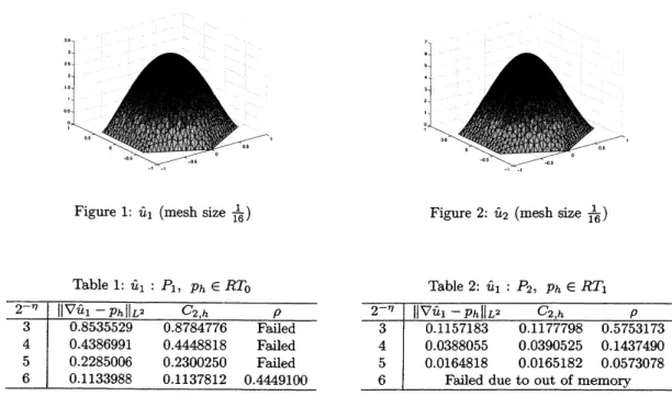
treat thefollowing modelproblem. Here,$\Omega$ isassumed to be hexagonal domain,

$\{\begin{array}{ll}-\triangle u=u^{2}+10, in \Omega,u=0, on \partial\Omega.\end{array}$

There

are

two approximate solutions $\hat{u}_{1},\hat{u}_{2}\in V_{h}$ given by finite element method. These

are

displayed in

Figure 1, 2 withthe mesh size $2^{-4}$_. For the first _approximate_solution

$\hat{u}_{1}$, verification results

are

shown in Table 1, 2. Here,

we use

$P_{1}$ (piecewise linear) and $P_{2}$ (piecewise quadratic) elements for getting $\hat{u}_{1}$

.

We adopt $RT_{0}$space for$P_{1}$-elementand$RT_{1}$ spacefor$P_{2}$-element.

Comparing two

cases

inTable 1 andTable2,

we

can

observe thathigherorderelements yield improved

result.

Figure 1: $\hat{u}_{1}$ (mesh size$\frac{1}{16}$)

Table 1: $\hat{u}_{1}$ : $P_{1},$ $p_{h}\in RT_{0}$

Figure 2: $\hat{u}_{2}$ (meshsize $\frac{1}{16}$)

Table 2: $\hat{u}_{1}$ : $P_{2},$ $p_{h}\in RT_{1}$

Next, wepresentresultswith respectto$\hat{u}_{2}$ whichis from$P_{2}$ finiteelementspace. InTable3, comparison of eachevaluation (14), (17) and (18) implies

our

proposed

one

workswell. Numericvalues

on

last columnin Table

3

express upper bound of absolute

error

$\rho$using (18) residual bounds. Based

on

Newton-Kantorovich

theorem,

we

prove that there is

a

solution in$\overline{B}(\hat{u}, \rho)$.

(7)

A

Notes

of

Raviart-Thomas elements

on

triangle

Inthispart,we would like to noterepresentationsof the lowest$(RT_{0})$ andlstorder $(RT_{1})$ Raviart-Thomas elementon

a

triangle element $K_{h}$

.

Vertices of$K_{h}$ are numbered

as

1, 2, 3. Theircoordinates

are

$(x_{1}, y_{1})$,

$(x_{2}, y_{2}),$ $(x_{3}, y_{3})$

.

Let

us

denote $a_{i}=x_{j}y_{k}-x_{k}y_{j},$ $b_{i}=y_{j}-y_{k}$, ci $=$ _xk–xj where $(i,j, k)$

are

even

permutationof(1,2,3). Here,

we

put subtense of each vertex

as

$e_{i}$ with direction from$j$to $k$

.

See

$K_{h}$ in

Figure

3.

Then it follows

3 $(X, Y)$

Figure

3:

Triangleelements$K_{h}$ and$\tilde{K}_{h}$

1 $x_{1}$ $y_{1}$ $1$ $x_{2}$ $y_{2}$

$1$

$x_{3}$ $y_{3}$

$|e_{i}|=(b_{i}^{2}+c_{i}^{2})^{1/2}$, _$D=$ 1 $x_{2}$ $y_{2}$ $=b_{j}c_{k}-b_{k}c_{j}$

.

Furthermore,the unit normal vector$n_{i}$

on

each side is givenby

$n_{i}=(n_{2}^{(i)}n_{1}^{(i)})= \frac{-\sigma}{|e_{i}|}(\begin{array}{l}b_{i}c_{i}\end{array})$ , where$\sigma=D/|D|$ is corresponding tothedirection ofnumbering. Namely,

$\sigma=\{\begin{array}{ll}1, ( i,j, k : counter clockwise rotation),-1, ( i,j, k :clockwise rotation).\end{array}$

For $q\in RT_{k}(K_{h})$, degrees of freedom

are

givenby

$\int_{\partial K_{h}}q\cdot n\varphi_{k}ds$, $\varphi_{k}\in R_{k}(\partial K_{h})$, for $k\geq 0$, (19)

$\int_{K_{h}}q\cdot q_{k-1}ds$, $q_{k-1}\in(P_{k-1}(K_{h}))^{2}$, for$k\geq 1$

.

(20)

A.l

$RT_{0}$

element

For$Ph\in RT_{0}$, therepresentationof$RT_{0}$ element$p_{h}$ on

a

triangle$K_{h}$ is given by

$p_{h}|_{K_{h}}=(\begin{array}{l}\alpha_{1}\alpha_{2}\end{array})+\alpha_{3}(\begin{array}{l}xy\end{array})$

Let

us

explainhow to determine coefficients$\alpha_{i}$

.

Threefreedoms

are

given by the following form,which is equivalent to (19) in

case

of$k=0$

.

(8)

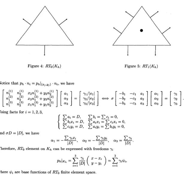
Figure4: $RT_{0}(K_{h})$ Figure5: $RT_{1}(K_{h})$

Notice that$p_{h}\cdot n_{i}=p_{h}|_{(x_{j},y_{j})}\cdot n_{i}$, we have

$[n_{1}^{(3)}n_{1}^{(2)}n^{(1)}1$ $n_{2}^{(3)}n_{2}^{(2)}n_{2}^{(1)}$ $x_{1}n_{1}^{(3)}+y_{1}n_{2}^{(3)}x_{3}n_{1}^{(2)}+y_{3}n_{2}^{(2)}x_{2}n^{(1)}1+y_{2}n_{2}^{(1)}]\{\begin{array}{l}\alpha_{1}\alpha_{2}\alpha_{3}\end{array}\}=[\gamma_{3/}\gamma_{2}\gamma_{1/}/|\begin{array}{l}e_{1}e_{2}e_{3}\end{array}|]$$\Leftrightarrow\sigma\{\begin{array}{lll}-b_{1} -c_{1} a_{1}-b_{2} -c_{2} a_{2}-b_{3} -c_{3} a_{3}\end{array}\}\{\begin{array}{l}\alpha_{1}\alpha_{2}\alpha_{3}\end{array}\}=\{\begin{array}{l}\gamma_{1}\gamma_{2}\gamma_{3}\end{array}\}$

.

Using factsfor$i=1,2,3$,

$\{\begin{array}{ll}\sum a_{i}=D, \sum b_{i}=\sum c_{i}=0,\sum b_{i}x_{i}=D, \sum a_{i}x_{i}=\sum c_{i}x_{i}=0,\sum c_{i}y_{i}=D, \sum a_{i}y_{i}=\sum b_{iy_{i}}=0,\end{array}$

and $\sigma D=|D|$,

we

have

$\alpha_{1}=-\frac{\sum\gamma_{i}x_{i}}{|D|}$, $\alpha_{2}=-\frac{\sum\gamma_{i}y_{i}}{|D|}$, $\alpha_{3}=\frac{\sum\gamma_{i}}{|D|}$

.

Therefore,$RT_{0}$ elementon$K_{h}$ canbe expressed with freedoms$\gamma_{i}$

$p_{h}|_{K_{h}}= \sum_{i=1}^{3}\frac{\gamma_{i}}{|D|}(\begin{array}{l}x-x_{i}y-y_{i}\end{array})=\sum_{i=1}^{3}\gamma_{i}\psi_{i}$, where$\psi_{i}$ are base functions of$RT_{0}$ finite element space.

Remark 4. The image

_of

$RT_{0}(K_{h})$ is given in Figure

4.

Further

for

$q\in(L^{2}(\Omega))^{2}$, let us

define

linear

functional, $F_{i}(q)=$

I

$e_{i}|\{q(x_{j}, y_{j})\cdot n_{i}\}(i=1,2,3)$

.

It

follows

$F_{i}(\psi_{j})=\delta_{ij}=\{\begin{array}{l}1, (i=j),0, (i\neq j),\end{array}$ _{$1\leq i,j\leq 3$}.

A.2

$RT_{1}$

element

Next let us consider lst order Raviart-Thomas finite element. Degrees of freedom

are

denoted by $\gamma_{i}\in$

$\mathbb{R}(i=1, \ldots, 8)$

.

For simplicity,

we

will transform triangle$K_{h}$to$\tilde{K}_{h}$,whichhas vertices

$(0,0),$ $(h, 0),$ $(X, Y)$

in Figure3.

$h=(b_{3}^{2}+c_{3}^{2})^{1/2}$, $(\begin{array}{l}XY\end{array})=\frac{1}{h}(\begin{array}{ll}c_{3} -b_{3}b_{3} c_{3}\end{array}) (\begin{array}{l}-c_{2}b_{2}\end{array})$ , $D=hY$,

$n_{1}= \frac{\sigma}{|e_{1}|}(\begin{array}{l}Y-(X-h)\end{array})$, $n_{2}= \frac{\sigma}{|e_{2}|}(\begin{array}{l}-YX\end{array})$, $n_{3}= \frac{\sigma}{|e_{3}|}(\begin{array}{l}0-h\end{array})$

.

In the following, we wouldliketo

exPlain

$RT_{1}$ element on$\tilde{K}_{h}$. _{$RT_{1}$} element

$p_{h}$is representedon

$\tilde{K}_{h}$,

(9)

Coefficients $\alpha_{i}$

are

obtained by the following method of determination with respect to$\gamma_{i}$

.

For$i=1,2,3$,

degrees of freedom

are

givenby (19) and(20),

$\int_{e}.Ph$ ni$\phi_{j}ds=\gamma_{i}$, $\int_{e}.Ph$ ni$\phi_{k}ds=\gamma_{i+3}$, $\int_{K_{h}^{-}}Ph$ $(\begin{array}{l}l0\end{array})ds=\gamma_{7}$, $\int_{K_{h}^{-}}P\hslash$ $(\begin{array}{l}0l\end{array})ds=\gamma s$, where $\phi_{j},$$\phi_{k}$ denote piecewise linear functions

on

$e_{i}$, satisfying $\phi_{j}(x_{j}, y_{j})=\phi_{k}(x_{k}, y_{k})=1,$$\phi_{j}(x_{k}, y_{k})=$

$\phi_{k}(x_{j}, y_{j})=0$

.

So

that

we

have

$\frac{\sigma}{6}|$ $-3Y-3Y3_{0}^{0}Y3YO6$ $Y(2X+h)Y(X+2h)2(X_{O}^{O}+h)-2_{0}XY-XY$ $-2Y^{2}-Y^{2}2Y^{2}2Y\gamma_{0}^{2}00$ $-3(X–3(\overline{x_{0}^{3h}-}3h3_{6}X^{-}3Xh)h)$ $-(x_{2x_{4^{2X+h)}}^{2}}-h)(X+2h)-t^{x-h)}2(X^{O}+h)-2h^{2}-h^{2}X$ $-2(x_{0}^{0}-h)Y-(Xh)Y2XYXY2Y0$ $h^{2}h^{0}(2^{+x+X^{2}}X+^{0}h)Y/2hY(2x+h)hY(x_{0}+2h)0$ $(2X+^{O}h)Y/22h_{0}^{O}Y^{2}hY^{2}Y^{2}0$ $|$ $|\begin{array}{l}a_{1}\alpha 2\alpha 3\alpha 4a_{5}\alpha 6a_{7}\alpha 8\end{array}|$$=|\begin{array}{l}\gamma_{l}\gamma_{2}\gamma_{3}\gamma_{4}\gamma_{5}2_{77}/D\gamma_{6}2\gamma_{8}/D\end{array}|$.

Solvingabove linear system,

we

havethevalue of each coefficients. Then, $RT_{1}$ elementisdescribed

on

$\overline{K}_{h}$,

$p_{h}|_{K_{h}^{-}}= \sum_{i=1}^{8}\gamma_{2}\psi_{i}$,

where$\psi_{i}$

are

base functions

as

following

Remark 5. See Figure 5

_for

degrees

_of

_freedom

to $RT_{1}(\tilde{K}_{h}).$ A linear

functional

is

defined

by $F_{i}(q),$ $(i=$

$1,$

$\ldots,$$8)$

for

$q\in(L^{2}(\Omega))^{2}$, such that

$fi(q)=$

51

$q\cdot n_{l}\phi_{m}ds$, $f\iota_{+3}(q)=\int_{e_{l}}q\cdot n_{l}\phi_{n}\$, $F_{7}(q)= \int_{K_{h}^{-}}q\cdot(\begin{array}{l}l0\end{array})dx$, $F_{8}(q)= \int_{K_{h}^{-}}q\cdot(\begin{array}{l}01\end{array})dx$

(10)

References

[1] M. T. Nakao,A numericalapproachtothe proofof existence of solutions for elliptic problems, Japan

Journal of AppliedMathematics,

5

(1988), pp.313-332.

[2] M.T. NakaoandY.Watanabe,Numericalverffication methods for solutionsofsemilinear elliptic

bound-ary valueproblems, NOLTA, IEICE, Vol.E94-N, No. 1 pp.2-31, 2011.

[3] M. Plum, Explicit $H_{2}$-estimates and pointwisebounds forsolutions ofsecond-orderelliptic boundary

vaJueproblems, JournalofMathematical Analysis andApplications, 165 (1992), pp.36-61.

[4] M. Plum, Computer assisted proofs for semilinear elliptic boundary valueproblems, Japan Journal of

Industrial and AppliedMathematics, 26 (2009), pp.419-442.

[5] P. Deuflhard and G. Heindl, Affine Invariant Convergence Theorems for Newton$s$ Method and

Ex-tensions to Related Methods, SIAM Journal

on

Numerical Analysis, vol.16, no.1, pp. 1-10, February

1979.

[6] L. V. Kantorovich and G.P.Akilov, Functional Analysis in Normed Spaces, translated from the Russian

by D. E. Brown, Pergamon Press, (1964).

[7] P. Grisvard, Elliptic Problems in NonsmoothDomain, Pitman, Boston, (1985).

[8] M.T. Nakao, T. Kinoshita,Someremarksonthebehaviourof thefiniteelementsolutioninnonsmooth

domains, AppliedMathematics Letters 21, 12 (2008),pp.1310-1314.

[9] P.A. Raviart and J.M. Thomas, Introduction\’a1‘AnalyseNum\’erique des Equations

aux

D\’erivees

Par-tielles, Masson, (1983).

[10] D. Braess, Finite elements-Theory, fast solvers, and applications in solid mechanics-, Third Edition,

CambrideUniversity Press, 2007.

[11] F. Brezzi and M. Fortin, Mixed and Hybrid Finite ElementMethods, Springer-Verlag, (1991). [12] X. Liu and S. Oishi,Verified eigenvalue evaluation for elliptic operator onarbitrary polygonal domain,

prepare to publication.

[13] N. Yamamoto and M.T.Nakao, Numerical verifications for solutions toelliptic equationsusingresidual

equationswith

a

higher orderfiniteelement, Journal of Computationaland Applied Mathematics,

60

(1995), pp.271-279.

[14] A. TakayasuandS.Oishi,Amethod of computerassistedprooffor Nonlinear two-point boundary value problems using higher order finite elements, NOLTA, IEICE, Vol.E94-N, No.1 (2011), pp.74-89.

[15] F. Kikuchi and H. Saito, Remarks

on a

posteriori

error

estimation for finite element solutions, Journal of Computational and Applied Mathematics, 199 (2007), pp.329-336.

[16] S.M. Rump, INTLAB-INTerval LABoratory, in Tibor Csendes, editor, Developments in Reliable

Computing, Kluwer AcademicPublishers, Dordrecht (1999),pp.77-104.

[17] Gmsh: a three-dimensional finite element mesh generatorwith built-in pre- and post-processing