Non-monotone Spectral Projected Gradient Method for Semidefinite Program with Log-Determinant and $\ell_{1}-$1Norm Terms (New Trends of Numerical Optimization in Advanced Information-Oriented Society)

全文

(1)22. Non‐monotone Spectral Projected Gradient Method for Semidefinite Program with ಚ‐Determinant and \ell_{1} ‐Norm Terms Takashi Nakagaki,Mituhiro Fukuda, Makoto Yamashita Department of Mathematical and Computing Science Tokyo Institute of Technology. Sunyoung Kim Department of Mathematics Ewha W. University. Abstract. A variant of the spectral projected gradient (SPG) method proposed by Birgin, Martinez and Raydan is proposed to solve semidefinite programs with \log ‐determinant and \ell_{1} ‐norm terms. The SPG is modified in the orthogonal projection of the iterates onto the convex feasible set in order to obtain a cheap computation. Numerical results on the problems considered in the literature confirm that the implementation of the proposed method can be comparably faster than other well‐known methods for similar problems.. 1. Introduction. Let. x. be an. n. ‐dimensional random variable following a Gaussian distribution \mathcal{N}(x;\mu, \Sigma) . We. frequently are in situations where we want to estimate the mean \mu and the covariance matrix x^{(m)} are i.i. d . samples from this distribution, the distribution. If x^{(1)}, x^{(2)}, \hat{\mu}. := \frac{1}{m}\sum_{i=1}^{m}x^{(i)}. and. \hat{\Sigma}. \Sigma. of. := \frac{1}{m}\sum_{i=1}^{m}(x^{(i)}-\hat{\mu})(x^{(i)}-\hat{\mu})^{T}. are candidates for this mean and covariance matrix, respectively, if m\gg n . In the case m<n, we need to impose some “structure” or conditions over the covariance matrix to estimate it. The. Gaussian graphical models [5] and sparse covariance selection [3] are one of classical solutions, where problems such as. \begin{ar ay}{l \max-tr(\hat{\Sigma}X)+\log\detX s.t X_{ij}=0,(i j)\in\Omega\subset q\{1,2 n\}^{2} X\suc O, \end{ar ay} where X\succ O means that. X. is a symmetric positive definite matrix, or. \begin{ar ay}{l} \max -tr (\hat{\Sigma}X)+\log\det X-\rho\Vert X\Vert_{1} s.t X\suc O, \end{ar ay} are solved for a regularizing parameter \rho>0 . See d’Aspremont et al. [2] or Yuan and Lin [15] for early discussion on the relation between these two problems. In this short note, we consider the extension of the above problems:. () \mathcal{P}. \begin{ar ay}{l} \min f(X) :=tr(CX)-\mu\log\det X+tr(\rho|X|) s.t \mathcal{A}(X)=b, X\suc O, \end{ar ay}. where C, X, \rho\in \mathbb{S}^{n} , the space of n\cross n real symmetric matrices, |X|\in \mathbb{S}^{n} the matrix obtained by taking the absolute value of every element X_{\dot{i}j}(1\leq i, j\leq n) of X , and \mathcal{A} a linear map.

(2) 23 of \mathbb{S}^{n}arrow \mathbb{R}^{m} .. In (\mathcal{P}), C, \rho\in \mathbb{S}^{n}, \mu>0, b\in \mathbb{R}^{m} , and the linear map \mathcal{A} given by \mathcal{A}(X)= A_{m}\in \mathbb{S}^{n} , are given data.. (tr(A_{1}X), tr(A_{2}X), \ldots, tr(A_{m}X))^{T} , where A_{1}, A_{2}, The dual of ( \mathcal{P} ) is given by: ( \mathcal{D} ). \{\begin{ar ay}{l} \max g(y, W) :=b^{T}y+\mu\log\det(C+W-\mathcal{A}^{T}(y) +n\mu-n\mu\log\mu s.t. (y, W)\in \mathcal{F}, \end{ar ay}. :=\overline{\mathcal{W} \cap\hat{\mathcal{F} ,\hat{\mathcal{W} :=\mathbb{R}^{m}\cross \mathcal{W},\hat{\mathcal{F} :=\{(y, W)\in \mathbb{R}^{m}\cross \mathbb{S}^{n}|C+W-\mathcal{A}^{T}(y)\succ O \}, :=\{[W]_{\leq\rho} : W\in \mathbb{S}^{n}\} , and finally, for matrices W, \rho\in \mathbb{S}^{n}, [W]_{\leq\rho} is the matrix whose (i, j)th element is \min\{\max\{W_{ij}, -\rho_{ij}\}, \rho_{\dot{i}j}\}.. where \mathcal{F}. \mathcal{W}. We propose a variation of the projected gradient method originally presented by Birgin et al.. [1] to the dual problem ( \mathcal{D} ) . In order to apply our method, we assume three conditions on ( \mathcal{P} ) and A_{m} is linearly independent; (ii) The problem ( \mathcal{D} ) : (i) \mathcal{A} is surjective, i. e., the set of A_{1}, A_{2}, ( \mathcal{P} ) has an interior feasible point, i. e., there exists X\succ O such that \mathcal{A}(X)=b; (iii) A feasible point for ( \mathcal{D} ) is given or can be easily computed. i. e., there exists y\in \mathbb{R}^{m} and W\in \mathbb{S}^{n} such that |W|\leq\rho and C+W+\mathcal{A}^{T}(y)\succ O . These assumptions are not strong as many applications satisfy these assumptions with slight modifications.. Many approximate solution methods for solving variants of ( \mathcal{P} ) have been proposed over the years. Lu [8] was one of earliers who considered a systematic approach to solve this problem as an mathematical optimization problem. The subsequent Adaptive Spectral Gradient (ASPG) method and the Adaptive Nesterov’s Smooth (ANS) method [9] are one of the earlier methods which can handle large‐scale problems. Ueno and Tsuchiya [11] proposed a Newton method by localized approximation of the relevant data. Wang et al. [13] considered a primal proximal point algorithm which solves semismooth subproblems by the Newton‐CG iterates. Employing the inexact primal‐. dual path‐following interior‐point method, Li and Toh in [6] demonstrated that the computational efficiency could be increased, despite the known inefficiency of interior‐point methods for solving. large‐sized problems. Yuan [16] also proposed an improved Alternating Direction Method (ADM) to solve the sparse covariance problem by introducing an ADM‐oriented reformulation. For a more. general structured models/problems, Yang et al. [14] enhanced the method in [13] to handle block structured sparsity, employing an inexact generalized Newton method to solve the dual semismooth subproblem. They demonstrated that regularization using \Vert . \Vert_{2} or \Vert . \Vert_{\infty} norms instead of \Vert . \Vert_{1}. in ( \mathcal{P} ) are more suitable for the structured models/problems. Wang [12] first generated an initial point using the proximal augmented Lagrangian method, then applied the Newton‐CG augmented. Lagrangian method to problems with an additional convex quadratic term in ( \mathcal{P} ) . Li and Xiao [7] employed the symmetric Gauss‐Seidel‐type ADMM in the same framework of [13]. A more recent work by Zhang et al. [17] shows that ( \mathcal{P} ) with simple constraints as X_{ij}=0 for (i, j)\in\Omega can be converted into a more computationally tractable problem for large values of \rho . Among the methods. mentioned here, only the methods discussed in [13, 14, 12] can handle problems as general as ( \mathcal{P} ) . In here, we consider a modification of the non‐monotone spectral projected gradient method. originally proposed by Birgin et al. [1] over the ( \mathcal{D} ) which guarantee a superior performance than applying directly to the primal problem ( \mathcal{P} ) . A detailed description of the method and its conver‐ gence can be found in [10]. The main difference with the original Birgin et al.’s method lays in the projection of the next iterate. In there, the next iterate is orthogonally projected onto a closed convex set. In our method, we do not perform an exact projection. We define the next iterate, which should satisfy a non‐monotone Armijo condition, by first projecting the next iterate over a. box‐type constraint \hat{\mathcal{W} and then approximately project over an Linear Matrix Inequality (LMI) constraint \hat{\mathcal{F} . These projections are cheaper than performing an orthogonal projection over the. intersection of these two convex sets \hat{\mathcal{W} \cap\hat{\mathcal{F} which corresponds to our feasible convex set \mathcal{F}. In the next section, we describe our algorithm, the results concerning the stopping criterion and its convergence. In Section 3, we show the performance of the implemented algorithm, DSPG compared to some well‐known codes. Finally, Section 4 has some concluding remarks..

(3) 24 2. The Non‐Monotone Spectral Projected Gradient Method for the Dual Problem and its Convergence. The variant of the non‐monotone spectral projected gradient method over the dual problem ( \mathcal{D} ). is described in the following algorithm, where the notation X^{k} :=X(y^{k}, W^{k})=\mu(C+W^{k}+ \mathcal{A}^{T}(y^{k}))^{-1} is used. Therefore, once the approximate solution of the dual (y^{k}, W^{k}) is computed, the approximate solution of the primal problem X^{k} can be recovered. Also, P_{S} denotes the projection onto a closed convex set S :. P_{S}(x) := \arg\min||y-x||, y\in s. and. \nabla g(y, W) := (\nabla_{y}g(y, W), \nabla_{W}g(y, W)) = (b-\mu \mathcal{A}((C+W-\mathcal{A}^{T}(y))^{-1}), \mu(C+W-\mathcal{A}^{T}(y) )^{-1}) = (b-\mathcal{A}(X(y, W)), X(y, W)). .. Algorithm 2.1 (Dual Spectral Projected Gradient Method) Step. 0:. Set parameters \epsilon\geq 0, \gamma\in(0,1), \tau\in(0,1), 0<\sigma_{1}<\sigma_{2}<1,0<\alpha_{\min}<\alpha_{\max}<\infty and an integer parameter M\geq 1 . Take the initial point (y^{0}, W^{0}) which satisfy condition (iii), and. an initial projection length \alpha^{0}\in[\alpha_{\min}, \alpha_{\max}] . Set an iteration number. k :=0.. Step 1: Compute a search direction (a projected gradient direction) for the stopping criterion. (\triangle y_{(1)}^{k}, \triangle W_{(1)}^{k}) := P_{\overline{\mathcal{W}}} ((y^{k}, W^{k})+\nabla g(y^{k}, W^{k}))-(y^{k}, W^{k}) = (b-\mathcal{A}(X^{k}), [W^{k}+X^{k}]_{\leq\rho}-W^{k}) . If. | (\triangle y_{(1)}^{k}, AW_{(1)}^{k})| _{\infty}\leq\epsilon ,. stop and output. (y^{k}, W^{k}). (1). as the approximate solution.. Step 2: Compute a search direction (a projected gradient direction). (\triangle y^{k}, \triangle W^{k}) := P_{\overline{\mathcal{W}}}((y^{k}, W^{k}) +\alpha^{k}\nabla g(y^{k}, W^{k}))-(y^{k}, W^{k}) = (\alpha^{k}(b-\mathcal{A}(X^{k})), [W^{k}+\alpha^{k}X^{k}]_{\leq\rho}-W^{k}) .. (2). Step 3: Apply the Cholesky factorization to obtain a lower triangular matrix L such that C+W^{k}\mathcal{A}^{T}(y^{k})=LL^{T} . Let \theta be the minimum eigenvalue of L^{-1}(\triangle W^{k}-\mathcal{A}^{T}(\triangle y^{k}))L^{-T} . Then, compute. \overline{\lambda}^{k}:=\{ begin{ar ay}{l} 1 (\theta\geq0) \min\{1,-\frac{1}{\theta}\cros \tau\} (\theta<0) \end{ar ay} and set. \lambda_{1}^{k} :=\overline{\lambda}^{k}. Set an internal iteration number j :=1.. Step. 3a :. Set (y_{+}, W_{+}). Step. 3b :. If. :=(y^{k}, W^{k})+\lambda_{j}^{k}(\triangle y^{k}, \triangle W^{k}) .. g(y_{+}, W_{+}) \geq 0\leq h\leq m\dot{ \imath} n\{k,M-1\}m\dot{ \imath} ng(y^{k-h}, W^{k-h})+\gamma\lambda_{j}^{k}\nabla_{y}g(y^{k}, W^{k})^{T}\triangle y^{k} +. tr. (\nabla_{W}g(y^{k}, W^{k})\triangle W^{k}). is satisfied, then go to Step 4. Otherwise, choose and return to Step 3a.. \lambda_{j+1}^{k}\in[\sigma_{1}\lambda_{j}^{k}, \sigma_{2}\lambda_{j}^{k}] ,. and set j :=j+1,.

(4) 25 Step 4: Set \lambda^{k} :=\lambda_{j}^{k}, (y^{k+1}, W^{k+1}) :=(y^{k}, W^{k})+\lambda^{k} (Ayk, \triangle W^{k} ), (s_{1}, S_{1}) :=(y^{k+1}, W^{k+1})(y^{k}, W^{k}) and (s_{2}, S_{2}):=\nabla g(y^{k+1}, W^{k+1})-\nabla g(y^{k}, W^{k}) . Let b^{k}:=s_{1}^{T}s_{2}+tr(S_{1}S_{2}) . If b^{k}\geq 0 , set \alpha^{k+1}:=a_{\max} . Otherwise, let a^{k}:=s_{1}^{T}s_{1}+tr(S_{1}S_{1}) and set \alpha^{k+1}:= \min\{\alpha_{\max}, \max\{\alpha_{\min}, -a^{k}/b^{k}\}\}. Step 5: Increase the iteration counter. k. :=k+1 and return to Step 1.. The fact that above algorithm converges to the correct optimal solution can be found in [10]. In there, the most relevant results are that the optimality condition can be tested by the fixed point condition for an arbitrary step length \alpha>0[10] :. Lemma 2.2 (y^{*}, W^{*}) is optimal for ( \mathcal{D} ) if and only if (y^{*}, W^{*})\in \mathcal{F} and (3). P_{\overline{\mathcal{W}}}((y^{*}, W^{*})+\alpha\nabla g(y^{*}, W^{*}))=(y^{*}, W^{*}) for some. \alpha>0.. Also, as we can see from (2) that either the norm of the search direction (Ayk, \triangle W^{k} ). =. P_{\overline{\mathcal{W} }((y^{k}, W^{k})+\alpha^{k}\nabla g(y^{k}, W^{k}))-(y^ {k}, W^{k}) or the norm of the search direction for the step length \alpha^{k}=1 (1) (Ay_{(1)}^{k}, AW_{(1)}^{k})=P_{\overline{\mathcal{W}}}((y^{k}, W^{k})+\nabla g (y^{k}, W^{k}))-(y^{k}, W^{k}) can be used for the. stopping criterion. This fact is guaranteed by the following lemma [10]:. Lemma 2.3 The search direction (Ayk, \triangle W^{k} ) is bounded by. (Ay_{11)}^{k}, \triangle W_{(1)}^{k}) .. More precisely,. \min\{1, \alpha_{\min}\}| (\triangle y_{(1)}^{k}, \triangle W_{(1)}^{k}) ||\leq||(\triangle y^{k}, \triangle W^{k})| \leq\max\{1, \alpha_{\max}\} | (\triangle y_{(1)}^{k}, \triangle W_{(1)}^{k})| .. (4). Unfortunately, it is not possible to determine a complexity bound for the number of iterates. of the above algorithm. However, we can, similarly to the original SPG [1], prove the asymptotic convergence of Algorithm 2.1 [10]: Theorem 2.4 Algorithm 2.1 with \epsilon=0 stops in a finite number of iterations attaining the optimal value g^{*} , or generate a sequence \{(y^{k}, W^{k})\} such that. karrow\infty 1\dot{ \imath} m|g(y^{k}, W^{k})-g^{*}|=0. 3. Numerical Experiments. The implementation of Algorithm 2.1 is called DSPG in this section. We conduct numerical exper‐. iments of DSPG over some test problems considered in the literature [6]. For this purpose, the DSPG is compared with the inexact primal‐dual path‐following interior‐. point method (IIPM) [6], the Adaptive Spectral Projected Gradient method (ASPG) [9], the Adap‐ tive Nesterov’s Smooth method (ANS) [9], and the QUadratic approximation for sparse Inverse Covariance estimation method (QUIC) [4]. We note that different stopping criteria are used in each of the aforementioned codes. They obviously affect the number of iterations and consequently the overall computational time. For a fair comparison, we set the threshold values for the IIPM, ASPG, ANS, and QUIC comparable to that of DSPG. More precisely, the stopping criteria of the DSPG was set to. | (\triangle y_{(1)}^{k}, \triangle W_{(1)}^{k})| _{\infty}\leq\epsilon, where \epsilon=10^{-5} . For the IIPM, we employed \max. { \frac{gap}{1+|f(X^{k})|+|g(y^{k},W^{k})|} , pinf, dinf} gaptol: =10^{-6}, \leq.

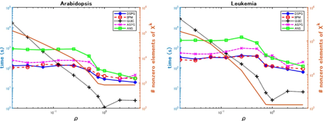
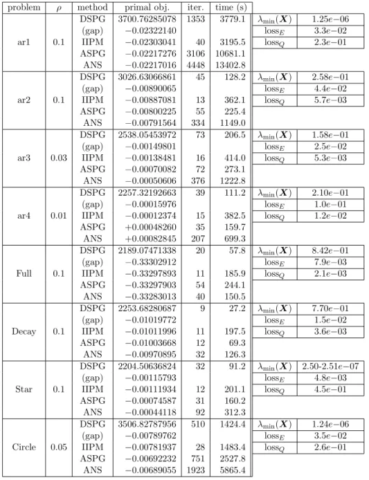
(5) 26 where gap, pinf, dinf were specified in [6], and for the ASPG and ANS, we used two thresholds \epsilon_{0} :=10^{-3} and \epsilon_{c} :=10^{-5} such that f(X)\geq f(X^{*})-\epsilon_{0} and \max_{(i,j)\in\Omega}|X_{ij}|\leq\epsilon_{c}[6] . The QUIC. stops when \Vert\partial f(X^{k})\Vert/Tr(\rho|X^{k}|)<10^{-6}. The DSPG was experimented with the following parameters: \gamma=10^{-4}, \tau=0.5,0.1=\sigma_{1}< \sigma_{2}=0.9, \alpha_{\min}=10^{-15}=1/\alpha_{\max}, \alpha_{0}=1 , and M=50 . In the DSPG, the mexeig routine of the IIPM was used to reduce the computational time. All numerical experiments were performed on a. computer with Intel Xeon X5365 (3.0 GHz) with 4S GB memory using MATLAB. We set the initial solution as (y^{0}, W^{0})=(0, O) , which satisfies the assumption (iii) for the instances tested in Subsections 3.1 and 3.2.. In the tables in Subsections 3.2, the entry corresponding to the DSPG under the column “pri‐. mal obj.” indicates the minimized function value ( \mathcal{P} ) for X^{k} , while “gap”’ means the maximized function value ( \mathcal{D} ) for (y, W) minus the primal one. Therefore, it should have a minus sign. The entries for the IIPM, ASPG, and ANS under “primal obj.” column show the difference between the corresponding function values and the primal objective function values of the DSPG. Thus, if this value is positive, it means that the DSPG obtained a lower value for the minimization problem. The. tables also show the minimum eigenvalues for the primal variable, the number of (outer) iterations, and the computational time. In order to measure the effectiveness of recovering the inverse covariance matrix \Sigma^{-1} , we adopt. the strategy in [6]. The normalized entropy loss (1oss_{E}) and the quadratic loss (1oss_{Q}) are computed as. 1 oss_{E}:=\frac{1}{n}(tr(\Sigma X)\log\det(\Sigma X)-n) , 1oss_{Q}:=\frac{1} {n}\Vert\Sigma X-I\Vert, respectively. Notice that the two values should ideally be zero if the regularity term tr(\rho|X|) is. disregarded in ( \mathcal{P} ) . Some other numerical results on the DSPG can be found in the extended version of this re‐. port [10]. 3.1. Real Data Problems. Five problems from the gene expression data [6] were tested for performance comparison. Since it was assumed that the conditional independence of their gene expressions is not known, linear constraints were not imposed and \rho=\rho I in ( \mathcal{P} ) , where I denotes the identity matrix.. Figures 1‐3 show the computational time (left axis) for each problem when \rho is changed. As \rho grows larger, the final solution X^{k} (of the DSPG) becomes sparser, as shown in the right axis for the number of nonzero elements of. X^{k}.. We can observe from these five cases shown in Figures 1‐3 that DSPG is comparable to the IIPM in terms of the computational time. They depend on the value of the regularizing parameter \rho>0 . As expected, QUIC is faster on sparse problems (with \rho larger) and slow on dense problems. (with. \rho. close to zero). We can clearly see that its computational time is proportional to the number. 3.2. Synthetic data. of nonzero elements of the approximate solution X^{k}.. The numerical results on eight problems where A\in \mathbb{S}^{n} has a special structure such as diagonal. band, fully dense, or arrow‐shaped [6] are shown in Tables 1. For each. A,. a sample covariance. matrix C\in S^{n} is computed from 2n i.i.d. random vectors selected from the n ‐dimensional Gaussian distribution \mathcal{N}(0, A^{-1}) . In these experiments, we did not compared with QUIC. We can see from Table 1 that DSPG is the fastest code to obtain a similar precision, excepting the “arl”’ problem, the most difficult case. For this instance, IIPM is the winner..

(6) 27. s_{X}. \hat{\ve m}. =Eq. g\cross. *\circ. *\circ. \dot{fracmegE\o asubet\omga}{Phi\tsmle^{}=E\omega. \frac{omegE=a}{\omeg. \subetcir Nq)k\. \subetcirNlon\. \#. \rho. \rho. Figure 1: Computational time (the left axis) for the DSPG, IIPM, QUIC, ASPG, ANS on the problems (Lymph” (n=587) and “ER” (n=692) when \rho\in [0.015625, 4]; \# of nonzero elements of X^{k} for the final iterate of DSPG (the right axis).. x_{X}. g\cross. *\circ. *\circ. \frac{omegE=a}{\omeg. \dot{frac\PhiE \subetomga}{Q)\hat{smile^{}\nq. \hat{\smile^{\omega}. \underli {E\omega}. \subetcir NPhk\. 10. \rho. 1. 10^{0}. =. \subetcir=Nh. \#. 10. 1. 10^{0}. \rho. Figure 2: Computational time (the left axis) for the DSPG, IIPM, QUIC, ASPG, ANS on problems “Arabidopsis” (n=834) and “Leukemia” (n=1255) when \rho\in [0.015625, 4]; \# of nonzero elements of X^{k} for the final iteration of DSPG (the right axis)..

(7) 28. Table 1: Comparative numerical results for the DSPG, IIPM, ASPG and ANS on synthetic problems with n=2000.. 483106{\imath}e_{40r 13. 334. 16 376. 15 207. 11. 40. 11 12. 12. 19235_{8}^9210.

(8) 29. -x *\circ. \dot{fracvEmeg}\oa. \hat{\smile^{\omega}. =Ev. =\cirvh N. 10^{1} 10^{0}. \rho. Figure 3: Computational time (the left axis) for the DSPG, IIPM, QUIC, ASPG, ANS on the problem “Hereditary bc” (n=1869) when \rho\in [0.015625, 4]; \# of nonzero elements of X^{k} for the final iteration of DSPG (the right axis).. 4. Concluding Remarks. In this note, we have proposed a variant of the spectral gradient method applied to the dual problem of the semidefinite program with \log‐determinant and \ell_{1} ‐norm terms. The method is efficient in terms of computational time since it avoids to perform an orthogonal projection onto the convex feasible set. Instead, it executes two projections onto convex sets which maintains. feasibility. Convergence of the method can be proved [10]. The numerical experiments compared to similar codes show that it can be faster in some instances, specially compared to the state‐of‐art. IIPM [6]. For further work, we can consider extending methods to more general cases such as minimiza‐. tion of quadratic convex functions [12] or some block diagonal structure considered on the matrix variable [13, 14].. Acknowledgement M. F. research was partially supported by JSPS Grant‐in‐Aid for Scientific Research (C) No: 26330024, and by the Research Institute for Mathematical Sciences, a Joint Usage/Research Cen‐ ter located in Kyoto University. M. Y. research was partially supported by JSPS Grant‐in‐Aid. for Scientific Research (C) No:. 18K11176 .. And S. K. research was supported by NRF 2017‐. RlA2B2005119.. References. [1] E. G. Birgin, J. M. Martinez, and M. Raydan, “Nonmonotone spectral projected gradient methods on convex sets SIAM Journal on optimization, 10 (2000), pp. 1196‐1211. [2] A. d’Aspremont, O. Banerjee, and L. El Ghaoui, “First‐order methods for sparse covariance selection SIAM Journal on Matrix Analysis and Applications, 30 (2008), pp. 56‐66. [3] A. P. Dempster, “Covariance selection. Biometrics, 28 (1972), pp. 157‐175.. [4] C.‐J. Hsieh, M. A. Sustik, I. S. Dhillon, and P. Ravikumar, “QUIC: Quadratic approximation for sparse inverse covariance estimation Journal of Machine Learning Research, 15 (2014), pp. 2911‐2947..

(9) 30 [5] S. L. Lauritzen, Graphical Models, The Clarendon Press/ Oxford University Press, Oxford, 1996.. [6] L. Li and K.‐C. Toh, “An inexact interior point method for L_{1} ‐regularized sparse covariance selection Mathematical Programming Computation, 2 (2010), pp. 291‐315. [7] P. Li and Y. Xiao, “An efficient algorithm for sparse inverse covariance matrix estimation based on dual formulation Computational Statistics & Data Analysis, 128 (2018), pp. 292‐307. [8] Z. Lu, “Smooth optimization approach for sparse covariance selection optimization, 19 (2008), pp. 1807‐1827.. SIAM Journal on. [9] Z. Lu, “Adaptive first‐order methods for general sparse inverse covariance selection Journal on Matrix Analysis and Applications, 31 (2010), pp. 2000‐2016.. SIAM. [10] T. Nakagaki, M. Fukuda, S. Kim, and M. Yamashita, “Dual spectral projected gradient method for a \log‐determinant semidefinite problem Research Report, B‐490 Department of Mathe‐ matical and Computing Science, Tokyo Institute of Technology, 2018.. [11] G. Ueno and T. Tsuchiya, “Covariance regularization in inverse space the Royal Meteorological Society, 135 (2009), pp. 1133‐1156.. Quarterly Journal of. [12] C. Wang, “On how to solve large‐scale \log‐determinant optimization problems optimization and Applications, 64 (2016), pp. 489‐511.. Computational. [13] C. Wang, D. Sun, and K.‐C. Toh, “Solving \log‐determinant optimization problems by a Newton‐CG primal proximal point algorithm SIAM Journal on optimization, 20 (2010), pp. 2994‐3013.. [14] J. Yang, D. Sun, and K.‐C. Toh, “A proximal point algorithm for \log‐determinant optimization with group lasso regularization SIAM Journal on optimization, 23 (2013), pp. 857‐893. [15] M. Yuan and Y. Lin, “Model selection and estimation in the Gaussian graphical model Biometrika, 94 (2007), pp. 19‐35. [16] X. Yuan, “Alternating direction method for sparse covariance models Computing, 51 (2012), pp. 261‐273.. Journal of Scientific. [17] R. Y. Zhang, S. Fattahi, and S. Sojoudi, “Large‐scale sparse inverse covariance estimation via thresholding and max‐det matrix completion. (2018), pp. 5766‐5775.. Proceedings of Machine Learning Research, 80.

(10)