When is a Stokes Line not a Stokes Line? : I. The Higher Order Stokes Phenomenon (Recent Trends in Exponential Asymptotics)

When is

a

Stokes

Line not

a

Stokes Line?

I. The Higher

Order Stokes

Phenomenon

C.J.Howls

University ofSouthampton

November 30,

2004

1

Introductaon

The field ofexponential asymptotics deals with the inclusion ofexponentially small terms in

singular perturbative expansions. Suchterms wouldusually be neglectedforreasonsofnumerical

insignificance andaperceptionthat theircontribution toanexpansion is faroutweighed by the difficulty in their calcuiation. Work in the field ofexponential asymptotics over the past two

decadeshas shown thatthese Leading orderattitudes may not always be correct.

This is the first of three sequential articles dealing with a recent development in the field.

These papers arose from a lecture

course

given at the meeting Recent Trends in Emponential

Asymptotics at RIMS, Kyoto inJuly 2004.

It is worthrecalling briefly why

someone

might wish to modify an expansion of the form

$y( \mathrm{a})\sim\sum_{n=0}^{\infty}a_{n}(\mathrm{a})\epsilon^{n}$ (1.1)

toinclude exponentially small contributionsof the form

$y( \mathrm{a})\sim\sum_{n=0}^{\infty}a_{\mathrm{n}}(\mathrm{a})\epsilon^{n}+K\exp\{-\frac{f(\mathrm{a})}{\epsilon}\}\sum_{n=0}^{\infty}b_{n}(\mathrm{a})\epsilon^{n}$ (1.2)

where a$=$

{

$a_{1)}$a2,

..

.}

$a_{i}\in c$.

.

Thesmall exponentials

can

be used toremovethe ambiguities associated with the definition

ofaPoincare expansion.

2

.

Theinclusion of sm all exponentials

can remove

the confusion

over

the Stokes phenomenon,

whereby asymptotic expansions appear to change abruptty in form as a parameter (here

a or $\epsilon$) change smoothly

.

Depending on the size of $f(\mathrm{a})/\epsilon$ inclusion of an exponentially small term can increase

numerical accuracy ofthesolution.

.

Analytically, inclusion ofan exponentially small term $\mathrm{s}$ can be usedto increasethe range ofvalidity of the original approximationto regionswhere $e^{-f(a)/\epsilon}$ may be _$O(1)$

.

.

The presence of exponentialiy small terms is a consequence of the theory of resurgence

and provides additional information that aidsrigorous work

.

Terms that are initially exponentially

sm

all may actualiy grow to dominate

as

$a$ varies.

They are thus often keytounderstanding the stabilityofasystem.

Several introductory articles, covering the various approaches to the subject, have appeared

and, for example, aflavourofsoneof theseapproachescanbefound inpaperscontained within

Howls et $al$ (2000).

We shall be concerned with a developm ent that has

a

significance that spills over from the

cormnunity of researchers in asymptotics to wider areas of applied mathematics. Specifically

we shall discuss the existence, analysis and importance of the so-called “higher order Stokes

phenomenon”.

We shall discuss a variety of system$\mathrm{s}$that contain finite param eters a $=\{a_{1}, a_{2}, \ldots\}a_{i}\in c$ in

additionto the asymptoticvariable $\epsilonarrow$Q. For example the a-parameters maybe just asingle

spatialdimensions$x$or it mayrepresent spatio-temporalcoordinates$(x$,?$)$

.

Theasym ptotic

anal-ysisof thesesystems isnot onlyaffectedby the Stokes phenomenon, but alsobymore dramatic

coalescencephenomena where underlying singularitiesgenerating the asymptoticexpansions

co-alesceat caustics. Oncaustics thetermsthemselves in the simple asymptotic expansionsbecome

singular and

more

complicateduniformexpansionsarerequired. Suchcatastrophic effects have

been extensively studied asymptoticallyby (for example) Chester, et al. (1957), Berry (1969),

Olver (1974), Wong (1989), Berry

&

Howls $(1993, 1994)$ andare also well understood.

The surprising result of recent work is that knowledge of coalescences or Stokes phenomenon

aloneis not alwayssufficient to predict the asymptotic behaviour of functions in differentregions

ofa-space.

In the context of WKBsoiutionsof higherorderordinarydifferential equations it has beenknown

(Berketal 1982)that when

more

thantwopossible asymptoticbehavioursarepresent,so-called

“new Stokes lines” must be introduced to fully describe the analytic continuation (Aoki et $al$

1994, 2001, 2002). These “new Stokes lines” areactually ordinary Stokeslines,thatnevertheless

3

$\mathrm{i}\mathrm{i})$ along the Stokesline. Hence the Stokes line may evenvanishat finite andperfectly regular points ina-space,

The “higher order Stokes phenomenon” is one explanation ofthe mechanism for this change.

In the absence of knowledge of the existenceof a higher order Stokesphenomenon, it possible

to draw incorrect conclusions from a naive approach as to the existence of Stokes lines or

coalescences as onetraverses aspace.

As

we

shaltsee, thehigherorderStokesphenomenonismoresubtle than the Stokesphenomenon.

However its presence nevertheless canleadtothegeneration ofterms elsewhere in a-space that

can growto dominatethe asymptoticsand also affect whether

a

caustic phenomenoncanoccur

or not.

In this the first paper of the trilogy, we introduce the concept of the higher order Stokes

phe-nomenon

and the

reason

for it. In subsequent papers wedeal with the practicalities ofseeking

out thehigherorder Stokes phenomenonand its influence onreal-parameter situations, in

par-ticulartime evolution problem $\mathrm{s}$

.

Mostofthe ideas have alreadyappearedelsewhere (Howls et

at

2004, Chapman

&

Mortimer 2004). However herewe presentit in adifferent formtoemphasise

thebreadth ofapplication ofthe concept ofthe higher order Stokesphenomenon.

Hence in

52

ofthis paperwe introduce the higher order Stokesphenom enon (HOSP) by means

ofanexampleinvolvingasimplecanonical integral. Insection j3weshow how the higherorder

Stokes phenomenon is conveniently understood 1n terms of the remainder terms of asymptotic

expansions obtained viaa hyperasymptoticprocedure.

2The

Higher

Order Stokes Phenomenon in

a

Simple Integral

To illustratetheconcept ofahigher order Stokes phenomenon, weshall study the integral

$I( \epsilon;a)=\int_{C}\exp\{\epsilon^{-1} (\frac{1}{4}z^{4}+\frac{1}{2}z^{2}+az)\}dz$, (2.1)

where $C$ is a contour that starts at $V_{1}=\infty$exp$(-3\pi \mathrm{i}/8)$ and ends at $V_{2}=\infty\exp(\pi \mathrm{i}/\mathrm{S})$ and,

without loss of generality, $\epsilon$ is a small positive asymptotic parameter. The parameter

$a$ is a

complexvariable.

Using the definition

$f(z;a)=-( \frac{1}{4}z^{4}+\frac{1}{2}z^{2}+az)$ , (2.2)

therearethreesaddlepoints, $z_{0},$ $z_{1},$ $z_{2}$ which satisfy$df/dz=0$,that is

4

The pathsofsteepest descent throughthe saddles $z_{n}$ are the connectedpaths passing through

$z_{n}$ that satisfy

$C_{n}=\{z\in C : k\{f(z;a)-f_{n}(a)\}\geq 0\}$

.

(2.4)

The function $I(\epsilon;a)$ is related to the Pearcey function (Berry

&

Howls 1991). We choose this

integral toexplain the higher order Stakes phenonenon because it containsthe keyingredients

ofthe higher order Stokesphenomenon:

.

it contains 3 possible asymptotic contributions onefrom each of thesaddles;

.

these contributions dependon a (non-asymptotic) parameter$a$;

Furthermore, the integralnature allowsfor abettergeometric explanation of the phenomenon.

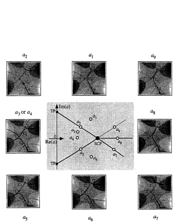
Wenowexamine the behaviour or theasymptotic expansionsas$a$varies smoothly in thecomplex

plane. First considerapoint $a=a_{1}$ infigure 1. The corresponding steepest descentpaths inthe

$z$-plane areshown in the samediagram in the box labeled

$a_{1}$

.

in thiscase we can take $C=C_{0}$

asthecontourofintegrationsothatonlythe saddle at $z_{0}$contributes to the$\mathrm{s}\mathrm{m}\mathrm{a}\mathrm{l}\mathrm{l}-\epsilon$ asymptotics

of$I(\epsilon;a)$

.

As wecross a Stokes curvein the a-plane definedby

$s_{i>_{J}}=\{a : \epsilon^{-1}(f_{j}(a)-f_{i}(a))>0\}$

.

_(2.5)

a Stokesphenomenonmay

occur

and the number of asymptoticcontributions may change. For

example, at$a=a_{2}$ which isapoint

on

sucha curve, the steepest descent contours of integration

is that part of$C_{0}$ that runs from $V_{1}$ to $z_{1}$ and the part of$C_{1}$ that runs from $z_{1}$ to $V_{2}$. Hence

an extra, _{exponentially subdominant, contribution from} $z_{1}$ is said to be switched on by the

dominant contribution from $z_{0}$

At $a=a\mathrm{s}$ the steepest descent contour of integration deform $\mathrm{s}$ to $C=C_{0}\cup C_{1}$. Hence saddles

at $z0$ and $z_{1}$ now both contribute to the small-c asymptotics.

Since the definition of Stokes

curves

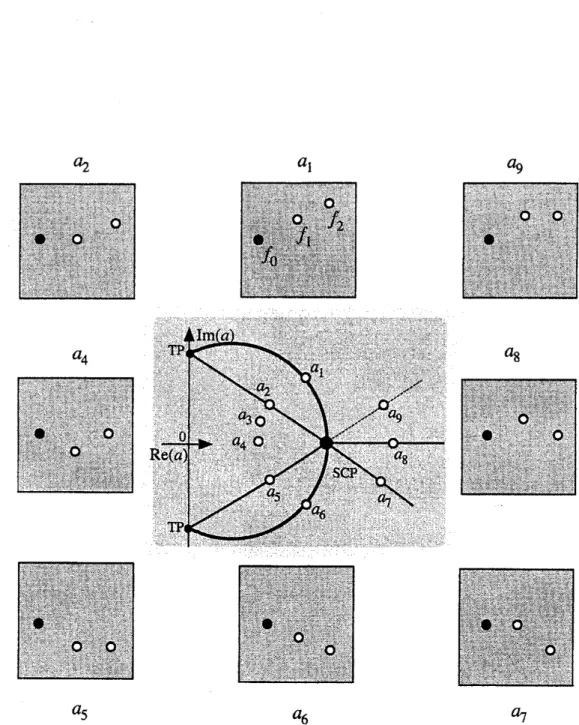
involves the values ofthe saddle heights it is convenient

to display the correspondingvalues $f_{j}(a)$ in the Borelplane (or complex $f$-plane) for the three

points_{above in figure 2. The form}ofthe mapping from the$z$ to $f$planeheregenerates

branch-cutsingularities at the images $f_{j}(a)$

.

TheBorelplanethuspossesses aRiemann sheet structure.

Thesteepest descent contoursmap tohorizontalloop contours startingand finishing at infinity,

encircling the corresponding saddlepoint-images. (Once the integral is written in an $f$-plane

representationit is possibleto deduce that it ispreciselythe presence of other suchsingularities

that is responsible for _{the divergence of the local asymptotic expansions about the} $f_{j}(a)$

see

e.g., Olde Daalhuis 1998, Howls 1991.) The main purpose ofplotting the Borel plane is that

$a_{2}$ $a_{1}$ $a_{9}$

$a_{5}$

$a_{6}$ $a_{7}$

Figure 1: The Stokes

curves

in the $a$ plane and the steepest descent contours of integration in

the integrand $z$-planepassing over saddles 0, 1 and 2 for selected values $a_{i}$ for integral (2.1).

The dashed Stokesline passing through $a_{9}$ is active, but irrelevant to the function defined by

$\epsilon$

$a_{2}$ $a_{1}$ $a_{9}$

$a_{5}$

$a_{6}$ $a_{7}$

Figure 2: Sketches ofthe Borel planes for (2.1) at values ofthe $a_{i}$ corresponding to those in

figure1. Ineach Borelplane thesolid dotis the image of saddle 0. The other dots

are

theimages

ofsaddles 1 and2. Ata Stokesphenomenontwoor moresoliddots

are

horizontally collinear

as

the steepest paths map to horizontallines. At

a

higher order Stokesphenomenon ($a_{1}$ and $a_{6}$)

threeor

more are

collinear in any direction. The higher order Stokes line is dravn in bold and

7

$f_{j}(a)$ passing through the horizontal contour of integration emanating from $f_{i}(a)$, to the right

of $f_{i}(a)$. Hence at $a_{2},$ $f_{1}(a)$ crosses the $\mathrm{b}\mathrm{r}\mathrm{a}\mathrm{n}\mathrm{c}\mathrm{h}-\mathrm{c}\mathrm{u}\mathrm{t}$emanatingfrom _{$f_{0}(a)$} this being the image

of$C_{0}$

.

To obtain the location of all the Stokes

curves

and hence deduce the asym ptotic expansion

in each sector of the complex $a$-plane it

seems

that all we have to do is to study the relative

alignment of the$fj(a)$ inthe complex $f$-plane. By consideration ofpoint $a4$, it is not difficult

to seethat this is not sufficient.

The steepest descent contours suggests that no Stokes phenomenonoccurs at $a_{4}$

.

However in

the Borelplane $f_{i}(a_{4})$, that$f_{2}(a_{4})$ isactually crossing the horizontal half-lineemanating from

$f_{0}(a_{4})$

.

Thus whenviewedin the$f$-planeaStokesphenomenonshould be occurring.

The resolution of this paradox is that although there is a branch point at $f_{2}(a_{4})$, when seen

from $f_{0}(a_{4})$ this branch point is not on the principal Riemann sheet. The saddle $z_{1}$ is “not

adjacent” to $z_{0}$ at $a=a_{4}$

.

Hence knowledge of the Riemann sheet structure ofthe Borelplane

is also required to establish whetheraStakes phenomenon takes place.

Continuinground in the a-plane,

we

see that at $a=a_{5}$ a Stakes phenomenon

occurs

between

saddles $z_{1}$ and $z_{2}$, so that when $a=a\epsilon,$ $C=C_{0}\cup C_{1}\cup C_{2}$ and aU three saddles contribute to

the $\mathrm{s}\mathrm{m}\mathrm{a}\mathrm{l}\mathrm{l}arrow\epsilon$asymptotics. At

$a=a7$

a

Stakes phenomenonswitches off thecontribution from $z_{1}$

so that $C=C\mathit{0}\cup C_{2}$ in the sector between a7 and$a8$

.

To completethe a-circuit back to $a_{1}$ we nownotice that the contribution from saddle$z_{2}$ must

be switchedoff since $I(\epsilon;a)$ single-valuedin $a$. This cannot

occur

at $a=a_{9}$, which is

a

typical

pointonthecontinuationofthe Stokes

curve

$S_{1>2}$, since saddle$z_{1}$ nolonger contributes to the

asymptotics of$I(\epsilon;a)$. Forthisreasonthe correspondingpartof that Stokescurveinthe central

box offigures 1 and 2 is dashed, since it is irrelevantfor the function defined by

our

choiceof

contour in (2.1). (It would have been relevant for

a

different choice ofvaUeys for the contour

of integration in (2.1)$)$

.

Hence another Stokes

curve

must be crossed somewhere

on

the circuit

between$a_{7}$and $a_{1}$

.

Consideration of the $f$-plane shows that

an

obvious choiceisat$a=a_{8}$, that

is as $f_{2}(a_{8})$

crosses

the horizontal half-line emanating from $f\mathrm{o}(a_{8})$. Thisis easily confirmed by

examinationof the steepestdescent paths in the box labeled $a_{8}$ in figure 1.

Having completed the circuit in$a$ space

we now

encounter asurprise.

The Stokes

curves

in the central box of figures 1 and 2 all

cross

at

a

particular point in the

a-plane, which we call the Stokes crossing point (SCP). In the analysis above

we

have shown

thatthe part of the positive real$a$-axis$(S0>2)$ from theoriginto theSCPis notanactive Stokes

curve, _Now we

see

_that the part of $S_{0>2}$ to the right of the SCP is

an

active Stokes curve.

When $a\in S_{0>2}$ is oneither

curve

in the corresponding $f$-plane, $f_{2}(a)$ is actually crossing the

horizontal$\mathrm{h}\mathrm{a}\mathrm{l}\mathrm{f}\sim \mathrm{l}\mathrm{i}\mathrm{n}\mathrm{e}$emanating from$f_{0}(a)$. Asmentioned above, for $a$to the left ofthe SCPthe

8

SCP it is.

To explain thechange in Riemann sheet structure we introduce theconcept ofa “higher order

Stokesphenomenon”that takes place

across

a new curveinthe complexa-plane passingthrough

the SCP that

we

calla “higherorder Stokes curve” (HSC).In theexample above, wehavechosen

$a_{1}$to lieon the HSC and fromfigure2

we see

that nothingofinterest happenshereto the steepest

descent paths. However in the complex $f$-plane, something significant is happening.

Let $a_{1}^{+}$ and$a_{1}^{-}$ be$a$-values slightly to theright and left of$a_{1}$ respectively. The values of$f_{J}(a)$

aredisplayed infigure3. It is clear from thisfigure thatat $a=a1,$ $f2(a)$isactuallycrossingthe

continuation of the line from$f_{0}(a)$ to $f_{1}(a)$

.

On theHSC $f\mathrm{o}(a),$ $f_{1}(a),$ $f_{2}(a)$

are

collinear in

the complex $f$-plane. When viewed ffom$f\mathrm{o}(a)$, this continuationofthe line is a radial branch

cut extendingfrom $f_{1}(a)$ (Olde Daalhuis 1998). Thus as colinearity of all three $f_{j}(a)$ occurs,

theRiemann sheet structure of the Borel plane in fact changes. For$a=a_{1}^{+}$ the point $f_{2}(a)$ is

on

the principalRiemann sheet

as

seen from$f_{0}(a)$, butfor $a=a_{1}^{-}$ it isnot. In the latter

case

to walk from $f_{0}(a_{1}^{-})$ to$f_{2}(a_{1}^{-})$

one

would first have to walk around$f_{1}(a_{1}^{-})$

.

A higher order Stokes phenomenon is thus said to

occur

when at least three of the $f_{j}(a)$ are

collinear in the$f$-plane. In turn, collinearityoccursat set ofpoints inthea-plane that wedefine

to be thehigher order Stakes

curve:

Higher Order Stokes Curve:

A higher order Stokes phenomenon takes place

across

a higher order Stokes curve, which is

defined by the set ofpoints:

$\frac{f_{j}(a)-f_{i}(a)}{f_{k}(a)-f_{j}(a)}\in R$

.

(2.6)

Wenowmake the followingobservations.

.

On a Stokes curve, at least two ofthe $f_{j}(a)$ differ by only

a

real number and

so

can be

joined by a horizontal line in the Borel-plane, Stokes

curves are

only active when the

relevant$f_{j}(a)$

are

onthe

same

Riemann sheet. SincetheRiemannsheet structure changes

as a higherorder Stokes

curve

is crossed, the activity ofa Stokes line (and therefore the

Stokes constants) changes

across

ahigher order Stokes

curve.

.

As

one

crosses

a Stokes line, an series prefactored by an exponential small term appears

(or disappears) in the fullexpansion. However

as one

crosses ahigher order Stokes

curve

there is

no

obvious such change in the asymptotic expansion. What has changed is the

existence ofa _{term in the remainder of the truncated expansion. This will be explained}

$a_{1}^{-}$ _{$a_{1}$} $a_{1}^{+}$

Figure3: Thehigherorder Stokesphenomenonin the Borelplanefor valuesof$a$

near

to$a_{1}$

.

At

the higher order Stokes phenomenon $f_{1}$ eclipses $f2$ when viewed ffom $f_{0}$

.

The Riemann sheet

structure of the Borel plane changes as $f_{2}$ passes through a radial cut from $f1$

.

At $a_{1}^{-},$ $f_{2}$ is

invisible from$f_{0}$ andso

no

Stokes phenomenon between $f_{0}$ and $f_{2}$

can

takeplace. At$a_{1}^{+},$ $f_{2}$ is

visible and

so a

Stokephenomenon isthenpossible.

.

Traditionally one expected that in the $a$-plane Stakes

curves

could only emanate from

turningpoints, where twoormore $f_{j}(a)$ coalesce,or ffomother singularities. However we

now seethat Stokes

curves

may start andendffomother regularpointsin the$a$-plane (the

SCP), where two or more other Stokes

curves

may

cross.

This effect has been observed

beforeby Berk et al (1982) andAoki et $al$ (1994, 2001, 2002).

.

It isimportant to note the differencebetween a Stokes

curve

being inactive and a Stokes

curve

being irrelevant. In the example above

no

Stokes curve hasbeen drawn between

$a=0$and the SCP.Nor hasonebeensketched from theSCP alongthe continuation ofthe

Stokes

curve

$S_{1>2}$in the directionof$a_{9}$

.

Jnthe first case aStokesphenomenoncould have

occurred, but it didn’t because $f_{2}(a)$ wasnot

on

the principal Riemann sheet

as

viewed

from$f_{0}(a)$ (i.e., they

were

not adjacent). This Stokes

curve

wastherefore inactive. In the

secondcase aStokesphenomenondoes in fact take place betweenthesaddles at$z_{1}$ and $z_{2}$.

However this particular phenomenon is irrelevant to the saddlepoint asymptotics of the

specific function $I(\epsilon$;a asdefined by

our

choiceof valleys in (2.1): in the neighbourhood

of this curve, $z_{1}$ is not contributing to the asym ptoticsof$I(\epsilon;a)$ anyway. If

we

had been

interested in a different function $\tilde{I}(\epsilon;a)$ defined by (2.1) but with $C$ running between

different valleys, then this

curve

could have been relevant whereas the first Stokes curve

would still be inactive.

.

At

a

higherorder Stokesphenomenonat least three of the$f_{j}(a)$arecollinear in the$f$-plane.

At a traditional Stokes phenomenon aminimum of onlytwoof the $f_{j}(a)$

are

required to

differbya real number. At

a

higher orderStokesphenomenonthere isnoactual constraint

on

the relative positioning of the first two $f_{j}(a)$ in the $f$-plane (a straight line canjoin

any twopointsinthea-plane). Hence atraditionalStokes

curve

and

a

higher-order Stokes

10

.

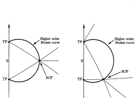
As the asymptotic parameter$\epsilon$changes inphase, the location ofStokes

curves

vary.

How-ever the colinearity condition that gives rise to the definition of a higher order Stokes

curve

isindependentof$\epsilon$

.

Thus the locationof the higher order Stokes curveisinvariant

under changes of the asymptotic parameter. This is illustrated in figure 4 for $\arg\epsilon=0$

and$\arg\epsilon=-\pi/4$.

.

Ahigher-orderStokes curvewillemanate from the

same

pointsastraditional Stokescurves.

Thesepoints are turningpoints

or

singularities of thephase function$f$

.

.

The concept ofahigher-orderStokescurvehasbeen couched above in terms ofasymptotic

expansions arisingfromsaddlepoint integrals. Howeversincewe haveexpressedeverything

in terms of the $f_{j}(a)$, theideas introduced are much

more

generally applicable. All that

is required to apply these definitions is the ability to determine all the different types of exponentialasymptoticbehaviours$\exp(-kf_{J}(a))$associated withanexpansion, regardless

of itsorigin. The only property peculiartothesaddlepoint integralthatwehave used above

isthe facilitytodeterminetheactivity of Stokescurvesfrom thesteepest descent contours

in the $z$-plane of the integrand. A more general way of achieving this is to compute the

“Stokes multipliers” $K_{ij}$. IfaStokes multipler has a zerovalue the corresponding Stokes

curveisinactive. Aslong

as

it ispossible tocompute the coefficients$T_{r}^{(J)}$ in theasym

ptotic expansions, thecomputation ofStokes multipliers is asolvedproblem, see OldeDaalhuis

(1998), Howls (1997) fordetails.

.

A higher-order Stokes curve requires collinearity of at least three $f_{j}(a)$. It is thus likely

to

occur

in any expansion that involves more than two different asymptotic behaviours

dependingon

a

set of additional parameters $\mathrm{a}$

.

A higher order Stakes phenomenoncould

thusoccurin expansions_{resulting from integrals involving threeor}

_more

_{criticalpoints (of}

any dimensionality), inhomogeneous second-order linear ordinary differential equations, higher order linearo.d.e.s, nonlinear o.d.e.s, and partial

differeriial

equations.

In the next section we give an explanation ofhow hyperasymptotic analysis is a natural way

to calculate not only the required Stokes multipliers in a more general problem, but also to

quantify preciselythe effects of

a

higher-order Stokesphenomenon.

3

Explanation

of

Higher Order

Stokes Phenomenon

The change in activity of Stokes linehas been noticed

or

discussed by several authors Berk et

al (1982), Aoki et al(1994, 2001, 2002), Chapman

&

Mortimer (2004). Here explain how and

why

a

higher order Stokesphenomenon gives rise to such

a

fundamental change in the analytic

structureof

an

expansion by_{reference to the exact remainder termsderivedby hyperasymptotic}

procedures (Berry

&

Howls 1991, Olde Daalhuis

&

Olver 1995,Howls 1997 Olde Daalhuis 1998

Figure4: The Stokes geometry for$\arg\epsilon=0$ (left) and$\arg\epsilon=-\pi/4$ (right). Thethin

curves

are

the normal Stokescurves,andthebold

curves

aretheHigherorder Stokescurves. Thisdiagram

is typicalof all theexampleswestudy in thistrilogy of papers.

contributions fromsimplesaddles. Howeverwhat followscanbe easily extendedtoanyfunction

thatpossesses aBorel transform.

Weshallstart from

an

integralinvolving theasymptotic parameter $6arrow 0$ of the form

$I^{(n\rangle}( \epsilon;\mathrm{a})=\int_{C_{n}\{\theta_{\mathrm{g}j}\mathrm{a}\}}e^{-f\langle z_{j}\mathrm{a})/\epsilon}g(z;\mathrm{a})dz$

.

(3.1)

We

assume

that $f$ possesses at least three saddlepoints situated at $z=z_{n}(n=0,1,2)$, where

$df/dz=0$. Again, we take $f_{n}=f_{n}(\mathrm{a})=f(z_{n};\mathrm{a})$

.

We

assume

that therangeofvalues of

a

are

such that the saddles aresimple so that$d^{2}f/dz^{2}\neq 0$, however this is a technical restriction to

simplify the discussion and

can

be removed later. The contour $C_{n}(\theta_{\epsilon};\mathrm{a})$ is then the steepest

descent path satisfying $\epsilon^{-1}\{f(z)-f_{n}\}>0$and running through (in general) a singlespecific

saddle at$z_{n}$, between specified asymptotic valleys of$\Re\{f(z) - f_{n}\}$ at infinity (deBruijn (1958)

$\mathrm{c}\}_{1}$

.

5, Copson (1965) $\mathrm{c}\mathrm{h}$. 7). The functions $f(z;\mathrm{a})$ and $g(z;\mathrm{a})$

are

analytic, at least in a

strip including $C_{n}(\theta_{\epsilon};\mathrm{a})$ and in the range of

a

values considered. As $\arg\epsilon$ varies, $C_{n}(\theta_{\epsilon\}}.\mathrm{a}]\backslash$

correspondingly deforms and for a set ofdiscrete values of$\arg\epsilon$it will encounter certain other

saddles $m$

.

These

are

called adjacent saddles, generating

an

additional contribution to the

asymptotics, prefactored by an exponentially small term: each of these births is

an

ordinary

Stokes phenomenon. Saddles that do not connect with $n$ as $\arg\epsilon$varies through $2\pi$

are

called

non-adjacent and do not (directly) generate

a

Stokes phenomenon.

Without loss of generality

we

order thelabelling ofthe saddles such that $\Re f\mathrm{o}<\Re f1<\Re f_{2}$for

12

avalue of

a

such that saddle 2 isadjacent to 1, butnot to 0.

We decompose the asymptotic expansion into the standard form ofa fast varying exponential prefactor anda slowlyvarying algebraicpart

$I^{(0)}(\epsilon;\mathrm{a})=\exp(-f\mathrm{o}(\mathrm{a})/\epsilon)\sqrt{\epsilon}T^{(0)}(\epsilon;\mathrm{a})$, (3.2)

(In the general case for

an

arbitrary Borel transform, the prefactor $\sqrt{\epsilon}$ will be replaced by an

arbitrary power $\epsilon_{0}^{\mu}$, say.) The algebraic part isexpanded

as

a

truncated asym ptoticexpansion

$T^{\{0\rangle}( \epsilon;\mathrm{a})=\sum_{\mathrm{r}=0}^{N0-1}T_{r}^{(0)}(\mathrm{a})\epsilon^{r}+R_{N_{0}}^{(0)}(\epsilon;\mathrm{a})$

.

(3.3)

By assumption$T^{(0\rangle}(\epsilon;\mathrm{a})$ is analyticin

$\mathrm{a}$

.

Consequentlyastraightforwardextension of the work

of Berry

&

Howls(1991) _{shows that the remainder term of this expansion may be written}exactly

as

$T^{\langle 0)}( \epsilon;\mathrm{a})=\sum_{r=0}^{N_{0}-1}T_{r}^{(0)}(\mathrm{a})\epsilon^{r}+\frac{1}{2\pi \mathrm{i}}\frac{K_{01}\epsilon^{N_{0}}}{F_{01}(\mathrm{a})^{N_{0}}}\int_{0}^{\infty}dv\frac{e^{-v}v^{N_{0}-1}}{1-v\epsilon/F_{01}(\mathrm{a})}T^{\langle 1)}(\frac{F_{01}(\mathrm{a})}{v};\mathrm{a})$ (3.4)

Here we have defined

$F_{nm}(\mathrm{a})=f_{m}(\mathrm{a})-f_{n}(\mathrm{a})$ (3.5)

is defined as the complex differencein heights between saddles $n$ and $m$. The factor $K_{01}$ is

effectively the Stakes constant relating to the contribution of saddle 1 to theexpansion about

saddle0, _{We recall that forexpansionsarising fromintegrals aStokesconstant}$K_{nm}$isreal with

modulusunityif$m$isadjacentto $n$andis

zero

otherwise,

as

explained_1n Howls(1997). In

more

generalcasesthe_{Stokes constant is a complex number.}

The term$T^{\{m)}$$($

.

.

.

$)$

on

theright hand side of (3.5)aretheslowlyvarying parts of integrals

over

the subset of theadjacent saddlesanalogous to theexpansion $T^{(0)}$

.

As$\epsilon$varies in phase, from the definitionof

a

Stokes phenomenon(2.5)between0and1canoccur

whenever $\arg(\epsilon/F_{01})$is

an

integer multiple of$2\pi$

.

At this phasethe exact remainder integral in

(3.4) encounters a poleon the real contour of integration. As the phaseof$\epsilon$ advances on, the

contour of integration of the remainderintegral (3.4) snags

on

thepole. In tur$\mathrm{n}$this introduces

a

residuecontribution (up to

a

sign):

$\frac{\epsilon K_{01}}{F_{01}(\mathrm{a})^{N_{0}}}{\rm Res}_{varrow F_{01}(\mathrm{a}\}/\epsilon}\{\frac{e^{-v}v^{N_{0}-1}}{1-v\epsilon/F_{01}(\mathrm{a})}T^{(1)}(\frac{F_{01}(\mathrm{a})}{v};\mathrm{a})\}=K_{01}e^{-F_{01}\{\mathrm{a})/\epsilon}T^{(1)}(\epsilon_{1}.\mathrm{a})$

.

(3.6)

When combined with the exponential prefactor $\exp(-f_{0}/\epsilon),$ $(3.6)$ produces

an

exponentially

small contribution$\exp(-f_{1}(\mathrm{a})/\epsilon)T^{(1)}(\epsilon;\mathrm{a})$

.

This is exactly the integral overthesteepest

con-tour $C_{1}(\theta_{\epsilon})$ passing through

13

As it stands, the exact remaindertermin (3.6) is implicit. In general weknow

no

more about $T^{(1)}$ than we did $T^{(0)}$

.

To circumvent this problem (Berry

&

Howls 1991) introduced

a

hy-perasymptotic appraoch: an expression for $T^{(1)}$, analogous to (3.4) can be written down by

inspection,in terms of its own adjacent terms

$T^{(1)}( \xi;\mathrm{a})=\sum_{r=0}^{N_{1}-1}T_{r}^{(1)}(\mathrm{a})\xi^{r}+\frac{1}{2\pi \mathrm{i}}\sum_{m=0,2}\frac{K_{1m}\xi^{N_{1}}}{F_{1m}(\mathrm{a})^{N_{1}}}\int_{0}^{\infty}dw\frac{e^{-w}w^{N_{1}-1}}{1-w\xi/F_{1m}(\mathrm{a})}T^{(m)}(\frac{F_{1m}(\mathrm{a})}{w};\mathrm{a})$ ,

(3.7) where $\xi=F_{01}(\mathrm{a})/v$. This corresponds to a $\mathrm{r}\mathrm{e}$-expansion ofthe remainder in the locality of saddle 1. Substitution of this expression into (3.4) generates a series of terms that can be

evaluated, together with a new implicit (and vith suitable choiceof$N_{0}$ and$N_{1}$) exponentially

smaller remainder. The newexpression is also valid in alarger sector,seeBerry

&

Howls 1991,

Olde Daalhuis

&

Olver 1995, Howls 1997or Olde Daalhuis 1998 for further details.

Thereare

now

two contributions to the remainder term of theoriginalexpansion(3.4) since 1 is

adjacenttoboth0and 2byassumption. The first is

a

“backscatter” contribution fromtheBorel

singularities correspondingto the saddles$\mathrm{f}i\mathrm{o}\mathrm{m}/\mathrm{t}\mathrm{o}0$via1. This contribution to the

rem

ainder of

the originalexpansionaboutfromsaddle0 containsnofurther potential singularitiesatthis first

level of$\mathrm{r}$ -expansion andso is not important for the argument here. However the contribution

fromsaddle 2, doescontain a further possiblesingularity, as wenowoutline.

We focus now on the exponentially smaller unevaluated remainder from the term involving

saddle 2. After substitution of (3.6) into (3.4) wediscoverit tobe ofthe form:

$R^{(012)}( \xi;\mathrm{a})=\frac{1}{(2\pi \mathrm{i})^{2}}\frac{K_{01}K_{12}\epsilon^{N_{0}}}{F_{01}(\mathrm{a})^{N_{0}-N_{1}}F_{12}(\mathrm{a})^{N_{1}}}$

$\mathrm{x}\int_{0}^{\infty}dv\frac{e^{-v}v^{N_{0}-N_{1}-1}}{1-v\epsilon F_{01}(\mathrm{a})}\int_{0}^{\infty}dw\frac{e^{-w}w^{N_{1}-1}}{1-wF_{01}(\mathrm{a})/vF_{12}(\mathrm{a})}T^{(2)}(\frac{F_{12}(\mathrm{a})}{w};\mathrm{a})$

.

(3.8)

$R^{(012)}$clearly hasapoie when the Stokesphenomenontakesplacewhere$F_{01}(\mathrm{a})/\epsilon>0$

.

It must

have this pole as it is a $\mathrm{r}\mathrm{e}$-expansion of the original remainder in (3.4) and so must contain

the Stokes phenomenon that was present in that exact remainder. However, ifais nowvaried

(independently from $\epsilon$), another potential pole in

$R^{(012)}$ can occurwhen

$F_{01}(\mathrm{a})/F_{12}(\mathrm{a})>0$. (3.9)

Note that this pole condition is identical to the colinearity condition (2.6). The

occurrence

of

the pole is therefore

synonymous

withahigher order Stokes phenomenon.

The residue from this poleis (upto a sign)

14

We

now

observethatas ahigher order Stokescurveiscrossed,apole arising in thehigherorder

hyperasymptoticremainder term switchesona

new

contribution to the remainder term.

Since $K01$ and $K_{12}$ are $\pm 1$, acomparison of the form of (3.10) with (3.4) and (3.7) shows that

this new contribution to be precisely the contribution to the remainderterm of the expansion

about 0 that one would expect ifsaddle 2 is adjacent to 0.

Note thatnowiftheparametersa (or$\epsilon$)arefurther varied suchthat$F_{02}(\mathrm{a})/\epsilon$becomes realand

positive then integration in the newremainder term (3.10) willencounter a pole and a Stokes

phenomenon wiilnowtakeplace between0 and 2. Prior to the higherorderStokesphenomenon

it could not.

Equally, we note that if0 and 2 mow coalesce so that $F_{02}(\mathrm{a})=0$ them the form of the

ex-pansion $(cf(3.10))$ breaks down and a caustic takes place. Prior to the higher order Stokes

phenom enon, althoughtheremay have been valuesofasuchthat$F_{02}(\mathrm{a})=0$, thecorresponding

Borel singularities wereactually vertically above each otheron differentRiemann sheets.

Thehyperasym ptotic approach has thus automatically carried out the accounting of all

contri-butions involved during the higher order Stokes phenomenon correctly, conciseiy and exactly.

The changes activity ofStokes lines can be traced to the changes in the presence ofterms in theexact remainder contributions. In turn thiscan thought ofasabrupt changes in the Stokes

constants themselves that prefactor theseremainder terms.

Finally, note that in a full hyperasymptotic theory, expressions for $T^{(j)}$ analogous to (3.7) can

be successively substituted into each implicit remainderterm, generating

a

tree like expansion

ofself-similiarmultiple integralcontributions calledhyperterminants (which

can

be

straightfor-wardly evaluated by the methods of Olde Daalhuis (1998b). Each such hyperterminant has a

denominator 1n the integrand of the form $1-wF_{ij}(\mathrm{a})/vF_{jk}(\mathrm{a})$ and

so a

higher order Stokes

phenom enonwili occurin any branch of thehyperasym ptotic expansion-tree whenever the

ap-propriate condition $F_{ij}(\mathrm{a})/F_{jk}(\mathrm{a})>0$issatisfied,

Consequently if there

are more

than 3singularities the aplane will be interweaved witha warp

and weft ofincreasingly higher order Stakescurves.

4

Conclusion

In thispaper we _{have introduced the higher order Stakes} phenomenonintermsofsystems that

havenatural integral representations. Wehaveusedahyperasymptoticapproachtoquantifythe

changes inactivityofStakeslines to changes in theRiemannsheet structure ofthecorresponding

Boreiplane. Otherexplanationsof the change inactivityofStokes linescertainly exist andcan

is

Inthe nextpaper of the trilogy wediscuss two examples in which we examine how to quantify

thehigherorder Stokes phenomenon inthe absence ofconvenient integral representations.

Acknowledgements

This work was supported by EPSRC grant $\mathrm{G}\mathrm{R}/\mathrm{R}18642/01$ and by a travel grant from the

Research Institute for Mathematial Sciences, UniversityofKyoto.

References

Aoki, T., Kawai, T.

&

Takei, Y. 1994New turning points in the exact WKB analysisfor higher

orderordinarydifferential equations. Analyse algebrique desperturbations singulieres, IMethods

resurgentes,Herman, pp 69-84.

Aoki, T., Kawai, T.

&

Takei,Y. 2001 On theexact steepestdescent method: a

new

method for

thedescription of Stokes curves, J. Math. Phys. 42, 3691-3713.

Aoki, T., Koike, T.

&

Takei, Y. 2002 Vanishing ofStokes Curves, in Microlocal Analysis and

Complex Fourier AnalysisEd Kawai. $\mathrm{T}$ andFujita K. (WorldScientific: Singapore).

Berk, H. L., Nevins, W. M.

&

Roberts, K. V. 1982 On the exact steepest descent method: a

new method for the description of Stokescurves. J. Math. Phys. 23, 988-1002.

Berry, M. V. 1969, Uniform approximation: a

new

concept in

wave

theory. Science Progress (Oxford) 57, 43-64.

Berry, M. V. 1989 Uniform asymptotic smoothing of Stokes’s discontinuities. Proc. R. Soc.

Lond. A 422, 7-21.

Berry, M. V.

&

Howls, C. J. 1991 Hyperasymptotics for integrals with saddles. Froc. R. Soc.

Lond. A 434, 657-675.

Berry, M. V.

&

Howls, C. J. 1993 Unfolding the high orders of asymptotic expansions with

coalescing saddles: singularity theory,

crossover

and duality. Proc. R. Soc. Lond. A 443,

i07-126.

Berry,M. V.

&

Howls, C. J. 1994Overlapping Stokes smoothings: survival of the

error

function

andcanonical catastropheintegrals. Proc. R. Soc. Loud. A444, 201-216.

18

Chester, C., Friedman, B.

&

Ursell, F. 1957 An extension ofthe method of steepest descents.

Proc. Cambridge Philos. Soc. 53, 599-611.

Delabaere, E.

&

Howls, C. J. 2002 Global asymptotics for multiple integrals with boundaries.

Duke Math. J. 112, 199-264.

Howls, C. J. 1992 Hyperasymptotics for integrals with finite endpoints, Proc. R. Soc. Lond. A

439, 373-396.

Howls, C. J. 1997 Hyperasymptotics formultidimensionalintegrals, exactremainderterms and

the globalconnectionproblem. Proc. R. Soc. Lond. A 453, 2271-2294.

Howls,C. J., Kawai, T.,TakeiY., 2000 Towards the exact WKBanalysis

_{of differential}

equations,

linear ornon-linear, (Kyoto University Press, Kyoto).

Howls, C. J., LangmanP., Olde Daalhuis A. B. , 2004 On the higher order Stokesphenomenon

Proc. R. Soc. Lond. A 460, 2585-2303.

OldeDaalhuis, A.B. 1998Hyperasymptoticsolutions ofhigher orderlineardifferentialequations

with asingularity of rankone. Proc. R. Soc. Lond. A 454, 1-29.

OldeDaalhuis, A. B.

&

Olver, F. W. J. 1995 Hyperasymptotic solutions ofsecond-order linear