CAN properties of the random-coefficient model of demand for nondurable consumer goods in the presence of national micro moments : A simulation study (Statistical Inference on Divergence Measures and Its Related Topics)

CAN

properties

of the

random-coefficient

model

of demand

for

nondurable

consumer

goods

in the

presence

of

national

micro

moments: A simulation

study

Yuichiro

KANAZAWA,

Ph.D.

1 _{Faculty of Engineering,Information,}

and Systems, UniversityofTsukuba

Kazuhiro NAKAYAMA

and Keisuke

TAKESHITA

Graduate SchoolofSystemsandInformationEngineering, University of Tsukuba

Abstract

Inthis paper, weimplement MonteCarlo simulation to examine asymptotic properties of the estimator of

random-coefficientlogitmodels ofdemand for non-durableconsumergoods underanequilibriumassumption

in the presence of micro moments

as

the numberoftheexamined regional markets increases. The national

micro moments

are

manufactured from the joint distribution of demographic information of

consumers

choosing those products with certain discriminating attributes. We observe that adding

an

equilibrium assumptionand the micro moments givesasymptotic normalitywithsharper asymptoticvariance-covariance

matrix,whilecorrecting asymptoticbiasreportedin Freyberger (2015). We discusspossible

reasons

for such

a

phenomenon.

$-d$

forScientificResearch $(B\rangle 16H0S333$,20310081, and the

Grant-in-Aid for Scientific ResearChfor Challenging ExplorateryResearch 25590051 from the Japan Society for the Promotion of

1

Introduction

Industrial organizationandsome marketingscience hterature isconcerned with the structure ofindustries

in the economy and thebehavioroffirmsandindividualsin theseindustries.

Suppose you observe high prices in

an

industry. We ask ourselves if this is due to market power,

or

due to high costs? Unfortunately, however,theimportant determinants of firmbehavior, costs,

are

usually

unobserved. The $u$

newempiricalindustrial organization” (NEIO;a moniker coinedby Bresnahan (1989))

is motivated bythis dataproblem. NEIO takesan indirect approach, in that weobtain estimate of firms’

market powerexpressed by markups by estimatingfirms’ demand functions.

Under NEIO, products

are

treated

as

bundlesof characteristics and preferences

are

defined

on

those

characteristics: Eachconsumerchoosesabundle thatmaximizesitsutility. Thischaracteristicsspace models

as

opposedto the

more

traditionalproduct space models solve ‘

too many paramete$r^{n}$ and

$u$

newgood$s^{n}$

problemsassoicated withthe latter.

Since

consumers

havedifferentpreferencesfor different characteristics,and hencemake different choices.

In this sense,

consumers are

heterogeneous. Thus we need to allow different

consumers

to have different

demographics-income,age,family size,location ofresidence,and other factors. Wethenformulateademand

systemwhichisconditional onthe$\infty$

nsumer

’

$s$characteristicsandavector ofparameterswhich determines

the relationshipbetweenthose characteristics andpreferences

over

products.

To formulate suchademand system usingmarket leveldata, weproceed

as

follows. First

we

draw

vec-tors of

consumer

characteristics from the distribution of thosecharacteristics,wethen determinethechoice

probability that each of the drawn households would make for a givenvalue of the parameter. Next we

aggregatethosechoice probabilities intoapredicted aggregatedemandconditionalonthe parametervector.

Finally

we

employ asearch routine to find thevalue ofthat parameter vector that makes these aggregate

probabilities

as

close

as

possible to the observed market shares. This idea ofsimulation estimators

devel-oped byPakes(1986) enabledusto “disaggregate”aggregatedemand to individual/household heterogeneous

behavioral modelin principle.

However, thereis a problem. Consumer goodsare differentiated inmany ways. As aresult

even

ifwe

econometricians measured alltherelevant characteristics, we could not expect to obtainprecise estimates

oftheir impacts. One solution proposed in Berry (1994) is to put in the $u_{importmt}n$ differentiating characteristicsandanunobservable,$\xi$, whichpicksuptheaggregate effectofthemultitudeofcharacteristics

thatarebeing omitted. Theunobservable$\xi$was thoughtto beburied deepinside ahighlynon-linear setof

equations,and hence it

was

not obvioushowtorecoverit. Berry (1994) showed thatthere isauniquevalue

for thevector of unobservables that makes thepredictedsharesexactlyequal totheobservedshares. Berry,

Levinsohn,and Pakes (1995;henceforthBLP(1995)) furtherprovidea contractionmapping techniquewhich

transformsthedemand system into

a

systemof equations thatislinear intheseunobservables.

consumers

as

well

as

producers: Consumers purchases products knowing $\xi$ and producers know $\xi$ when

they set prices. As a result, goods that have high values for $\xi$ will be priced higher in any reasonable

notion of equilibrium. This produces an a1zalogue to the standard simultaneous equation “endogeneity”

or (simultaneity problem in estimating demand systems in the older demand literature; i.e. prices are

correlatedwith the disturbance term. However, becauseofthe way theseunobservables

are

set upin BLP

(1995),we

are

ableto useinstruments toformulategeneraliled method ofmoments estimation (GMM for

short) to

overcome

this simultaneityproblem.”’

Somerecent empirical studies in industrial organizationand marketing science

ex

$\sqrt{}end$ the framework

proposed by Berry, Levinsohn and Pakes (1995, henceforth BLP (1995)) by integrating infomation on

consumer

demographicsintotheutilityfunctionsin order to make theirdemandmodels morerealisticand convincing.

Wide availability ofpublic

sources

ofinformation such as the Current Population Survey (CPS) and

the Integrated _{Public Use Microdata Series} (IPUMS) makes these studies possible. Those sources give

us information on the joint distribution ofthe U.S. household’s demographics including income, age of

household’shead,andfamily size. For example,Nevo$(2001\rangle$’sexaminationonprice competition in the_U.S.

ready-to-eatcereal industry

uses

individual’sincome, ageandadummyvariable indicating if$s/he$_{has a child}

in theutility_{function. Sudhir (2001) includes household’s incometomodel the U.S. automobiledemandin}

his studyofcompetitiveinteractions amongfirms in different market segments.

In analyzing the U.S. automobile market, Petrin (2002) goes further and links demographics of

new-vehicle purchasersto characteristicsofthe vehicles they purchased. Petrin adds a set of functionsofthe

expectedvalue of consumer’sdemographicsgiven specific product characteristics (e.g. expected familysize

ofhouseholdsthatpurchasedminivans)

as

additional moments to theoriginal moments usedin BLP (i995)

in theGMMestimation. Specifically,hematchesthemodel’sprobability ofnewvehiclepurchase fordifferent

income groups totheobservedpurchase probabilitiesin the ConsumerExpenditureSurvey(CEX)automobile

supplement. He also matches modelprediction for average household characteristicsof vehiclepurchasers

suCh

as

family-sizetothe data in CEXautomobile supplement. _{Petrin presupposes readily accessible and}

publicly available marketinformation

on

thepopulation

average.2

He maintains that “the extrainformation

plays the

same

role

as

consumer-leveldata, allowing estimated substitutionpatterns and (thus) welfare to

directlyreflectdemographic-drivendifferencesintastesforobserved characteristics” (page,706, lines22-25).

Hisintention, it$\Re ens$,is to reducethebias associated_{with “a heavy dependenceonthe idiosyncratic logit}

“taste”

error

(page707, lines 5-6).

Heexplains_{that “the idea for using theseadditionalmomentsderivesfromImbens and Lancaster(1994).}

Theysuggestthat _{aggregate data may contain usefulinformation}

_on

_{theaverageof micro variables” (page}

$-$

hand,uses detailedconsumepleveldata,which includenot onlyindividwals’

choices butalsothechoicesthey would have madehadtheirfirstchoiceproductsnotbeen available. Although the proposed

method shouldimprove theoutof-samplemodel’sprediction, it requires proprietaryconsumer-leveldata,whicharenot readily

availableto researchers,astheauthorsthemselvesacknowledged in the paper: theCAMIPdata “are generally notavailable to

713, lines

27-29

$)^{}$

It should be notedthat these additional momentsaresubjecttosimulation and sampling

errors

inBLP

estimation. This is because theexpectationsof

consumer

demographics

are

evaluatedconditional

on

aset

of exogenous productcharacteristics$X$ _andanunobservedproduct quality$\xi$, wherethe$\xi$is evaluated with

thesimulationerrorinducedbyBLP’scontractionmappingaswell

as

withthe samplingerrorcontainedin

observed market shares. In addition,market informationagainstwhichtheadditional moments

are

evaluated

itselfcontainsanother type of sampling

error.

Thisis becausethemarketinformation is typicallyanestimate

for the populationaverage demographics obtained from

a

sampleof

consumers

(e.g. CEX sample), while

observed market sharesare calculatedfromanothersampleof

consumers.

Thiserroralsoaffects evaluationof

the additional moments. In summary each ofthefourerrors (thesimulationerror, the samplingerrorinthe

observed market shares, the samplingerrorinduced when researcher evaluates the additionalmoments,and

thesampling

error

in the market

_information

itself)aswell

as

stochastic nature ofthe productCharacteristics

affects evaluation oftheadditional moments.

Theestimator proposed byPetrin appears toassume that we are abletocontrol impactsfromthefirst

fourerrors. However, it is notapparentif Petrin estimator is consistent andasymptotically normal (CAN)

without suchacontrol. Furthermore,it is not known either if how many andinwhat way individuals need

to besampled inorder forPetrinestimatorto be

more

efficientthan BLP estimator. Myojoand Kanazawa

(2012) formalized$Petrin^{)}s$_{idea andprovide}the conditionsunder which Petrin estimatornot onlyhasCAN

properties,butismoreefficient thanBLPestimator

as

the numberofproductsincreasesin

a

nationalmarket,

aframework designed to analyzedurable goods suchasautomobiles.

On the other hand, packaged goods such

as

foods, beverages, grooming aids, laundry powder, toiletries andothers

are

sold inaretail outlet whose shelf spaceislimited. Thus itisunrealistic for manufacturer to

increasethe numberof products andexpectretailers to carryall ofthem. Inaddition, shoppers forthose

packaged goods are likely to shop locally, so their prices are likelyto be determined in the local market.

Each one of these markets, of course, reflectsregional or local demographics, and thismay inducecertain

product characteristic(s) to be valued in

one

local/regional market, but not

so

much \’in the other. As

a

result,

consumers

in different markets may perceive the

same

product somewhat differently. To capture their heterogeneity forthoseproduct categories,we needto be able tohaveatooltoanalyzecircumstances

where thenumberof products is fixed, butwe

are

abletoobservemany of theselocal/regionalmarkets.

Reyberger (2015) develops asymptotic theory for estimated parameters in differentiated product

“de-mand” systemswithasmall number ofproductsand

a

largenumber of markets$T$

.

His asymptotictheory

takes intoaccountthefact that “the predictedmarketshares

are

approximatedbyMonte Carlo integration

with$R$draws and that theobservedmarket sharesareapproximated from asample of$N$$\infty$nsumers As

expected, he found “both approximations affect the asymptotic distribution, because they both lead to

a

3Originalintunsion ofImbensandLancasteris to improve efficiency foraclass of the extremum estimators. There isa

difference betweenPetrin’s and ImbensandLancaster’sapproaches in sampling process to construct original and additional

sample moments. Petrin combines thesample moments calculated over pnductswith additionalmoments calculated over

biasand a varianceterm in theasymptotic expansionof the estimator.” He showed that “when $R$ and $N$ do not increase faster than the numberof markets, the bias terms dominate the $vari\epsilon nce$ terms, _{and the}

asymptoticdistributionmight not be centeredat $0$andstandard confidence intervals do not have_{the right}

size, even asymptotically.” He showed that theleading bias terms canbe eliminated by usingananalytic

biascorrection method.

In this paper, we also deal with the same circumstances

as

Freyberger (2015) in which the number

ofproducts isfixed while the number of markets increases. We introduce the pricing equation

as

well

as

the additional micro moments orsummary statistics thatprovide

_information

on thejoint distribution

_of

consumer

demegraphicsandproduct_{characteristics}

_as

_Petrin (2002)and Myojo and Kanazawa(2012)did to

the model andinvestigate ifthe accuracy, bothintermsofbias and variance, of the estimator is improved

uponviaMonteCarlo simulation. Thisstudyis designed to facilitatetheoreticalexamination of theproblem.

2

System

_{of Demand and Supply with}

_{Additional Moments in}

Multiple Markets

Inthissection,wedefinethe product space precisely, andreframe theestimationprocedureof BLP (1995)

when combining the demand and supply side moments with the additional moments relating

consumer

demographics to the characteristics ofproducts they purchase. For convenience in comparison to Berry, Linton, and Pakes$\langle$2004) ($BI_{J}P(2004)$ forshort), notation and most definitions

arekeptas same

as

possible

tothoseinBLP (2004).

2.1

Demand

Side

Model

Regionalmarkets

are

indexedby$m=1$,$\cdots$,$M$andthepopulationin market$M$is$I_{m}$

.

We

assume

the

same

finite set of products,$j=1,$ $\rangle J$,is available in eachregionalmarket. We also

assume

that eachconsumer

onlyparticipates inone market andchooses

one

productincluding “outside” goodthat maximizes his/her

utilitywithin that market. We

assume

the utility of

consumer

$i$ for product$j$in regionalmarket $m$to be

$u_{ij}^{m} = \alpha\ln\langle y_{t}^{m}-p_{j}^{rn})+x_{j}’\beta+\xi_{j}^{m}+\sum_{k=1}^{K}\pi_{k}x_{jk}\nu_{ik}^{rn}+\epsilon_{ij}^{rn}$

(1) $= \alpha\ln(y_{i}^{m}-p_{j}^{m}\rangle+\sum_{k=1}^{K}x_{jk}(\beta_{k}+r_{k}\nu_{ik}^{rn})+\xi_{j}^{m}+\epsilon_{ij}^{\tau r\iota}.$

This specification closely parallels with that ofBLP (1995) except that some demographic and product

characteristics

are

indexed by$m$

as

well. For instance, $y_{i^{n}}^{7}$ is the income of

consumer

$i,$$p_{j}^{m}$ is the priceof

product $j,$ $\xi_{j}^{rn}$ is the unobserved product characteristics for product_$j,$ $\nu_{ik}^{m}$ is

consumer

$i$’s taste for k-th

productcharacteristic, and$e_{ij}^{rn}$is unobservedidiosyncratictastesof

consumer

$i$, all inmarket

$m$

.

We

assume

that $\epsilon_{ij}^{rn}$ arei.i.$d$with typeIextremevalue.

markettothe other because of thedifferences in demographicsbetween markets. However,

we

assume

the

parameters $(\alpha,\beta)$are notindexedby_$m.$

Althoughmost observedproductcharacteristics

are

not correlatedwith theunobservedproduct

charac-teristics $\xi_{j^{n}}’\in\Re,$ $j=1$,

.

.

.,$J$, some of them (e.g. price) are. We denote the vector ofobserved product

characteristics$x_{j}=(x_{1j}’, x_{2j}’)’$where$x_{1j}\in \mathfrak{R}^{K_{1}}$ areexogenousandnot correlatedwith$\xi_{j}^{m}$,while$x_{2j}\in \mathfrak{R}^{K_{2}}$

are

endogenousand correlated with $\xi_{j}^{m}$ where$K=K_{1}+K_{2}$

.

Observedproductcharacteristics other than

price, denoted as $x_{1j}$

are

not indexed by $m$ because we

assume

that the

same

set of products is sold in

every market. We

assume

the set of exogenousproduct characteristics $(x_{1j},\xi_{j}^{1},\xi_{j}^{2}, \ldots, \xi_{j}^{M})$,$j=1$,$\cdots$,$J$is

arandom sample from theunderlying populationofproduct characteristics, and is thusindependent

across

$j$ similar to the framework of BLP $(1995\rangle.$

The$\xi_{j}^{m\prime}s$areassumed to be

mean

independentof$X_{1}=(x_{11}, \ldots,x_{1J})’$

(2) $E_{\xi|X_{1}}[\xi_{j}^{rn}|X_{1}]=0$

with probability 1. Wealso

assume

theconditional variance of$\xi_{j}^{m}$on$x_{1j}$ is finite

$\sup \max E_{\zeta^{m}|x_{1j}}[(\xi_{j}^{m})^{2}|x_{1j}]<\infty$

$1\leq m\leq M^{1\leq j\leq J}$

with probabilityone. Wedenoteby$X=(x_{1}, \ldots, x_{J})’$ theset ofall observedproductcharacteristics.

We definethe utilityfor outsidegoodas

$u_{0}^{m}=\alpha\ln(y^{m})+\epsilon_{i0}^{m},$

andredefinethe utilityasdifference from outsidegood, $U_{1j}^{m}=u_{ij}^{m}-u_{i0}^{m}$ as

$U_{j}^{\dot{m}} = u_{1j}^{m}-u_{i0}^{m}$ $= \alpha\ln(y_{i}^{m}-p_{j}^{m})+\sum_{k=1}^{K}x_{jk}(\beta_{k}+\pi_{k}\nu_{ik}^{m})+\xi_{j}^{m}+\epsilon_{ij}^{m}-(\alpha\ln(y_{i}^{m})+\epsilon_{i0}^{m})$ $= \alpha\ln(1-\frac{p_{j}^{m}}{y_{1}^{m}})+x_{j}’\beta+\sum_{k=1}^{K}x_{jk}\pi_{k}\nu_{\grave{l}}^{m_{k}}+\xi_{j}^{m}+\epsilon_{ij}^{m}-\epsilon_{0}^{\dot{m}}$ (3) $= ff_{j}^{n}(x_{j},\xi_{j}^{m};\beta)+\mu_{ij}^{m}(x_{j},p_{j)}^{m}y_{1}^{m}, v_{i}^{m};\alpha,\pi)+\epsilon_{ij}^{m}-\epsilon_{/0}^{m},$ where $\delta_{j}^{m}(x_{j},\xi_{j}^{m};\beta) = x_{j}’\beta+\xi_{j}^{m},$

$\mu_{ij}^{m}(x_{j},p_{j}^{m},y_{i}^{m}, v_{l}^{\tau n};\alpha, \pi) = \alpha\ln(1-\frac{p_{j}^{m}}{y_{\dot{\iota}}^{m}})+\sum_{k=1}^{K}x_{jk}\pi_{k}\nu_{k}^{m}.$

This redefinition standardizes the utility function

so

that $U_{i0}=$ O. Note that $\delta_{j}^{m}(x_{i},\xi_{j}^{m};\beta\rangle$ depends on

The conditionalprobability$\sigma_{ij}^{m}$ forconsumer $i$inmarket$m$to chooseproduct$j$

(4) $\sigma_{ij}^{m}\langle X, \xi^{m}, y_{l}^{m}\prime, v_{i\rangle}^{m}\cdot\theta_{d})=\frac{\exp(\delta_{j}^{m}+\mu_{ij}^{m})}{\sum_{j=0}^{J}\exp(\delta_{j}^{m}+\mu_{ij}^{m}\rangle},$

is

a

map from the set of observed and unobserved product characteristics $X$ _and $\xi^{m}=(\xi_{1}^{m}, \ldots,\xi_{J}^{m})’,$

demographics$y_{i}^{\prime n}$ andtastes$v_{i}^{rn}\in \mathfrak{R}^{v}$of

consumer

$i$in market

$m$, and ademand parametervector $\theta_{d}\in\Theta_{d}.$

We

assume

$\sigma_{{\} j}^{m}\prime(X,\xi^{\nu n}, y_{i}^{rn}, v_{i}^{rn};\theta_{d})>0$for allpossiblevalues of$(X,\xi^{\tau n},y_{i}^{m}, v_{t}^{m};\theta_{d})$

.

The BLP framework generates the vector $\sigma^{m}$ of market

shares in region $m$ by aggregating

over

the

individuaJ choice probability $\sigma_{ij}^{m}$overthe joint distribution$P^{\prime n}(\cdot)$ofthe

consumer

demographics andtastes

$(y_{i}^{m}, v_{i}^{n})$

as

(5) $\sigma_{j}^{ln}(X,\xi^{m}, \theta_{d}, P^{m}\rangle=\int\sigma_{i_{\hat{J}}}^{rn}(X,\xi^{m}, y_{i)}^{rn}v_{i)}^{m}\cdot\theta_{d})dP^{m}(y_{i}^{m}, v_{i}^{m}\rangle$

where $P^{m}$ is typically the _{empiricaljoint distribution of the}

consumer

demographics and tastes from

a

randomsampledrawn from the underlyingpopulation jointdistribution$P^{m,0}$_{ofdemographics andtastesin}

market$m$

.

Ifweevaluate (5) at $(\theta_{d}^{0},P^{m,0})$, where$\theta_{d}^{0}$ is the true value ofdemand

sideparameters,wehave the “conditionallytrue” market shares $s^{m,0}$ _{giventhe product characteristics (X,}

$\xi^{rn}\rangle$ inmarket _$m$

.

That

is,

(6) $\sigma^{m}(X,\xi^{m},\theta_{d}^{0},P^{m,\zeta)})\equiv 8^{m,0}.$

where$s^{m, く)}=$$(s , \cdots, s_{J}^{\tau n,O})’.$

ffwesolvethe identity (6)atany$(\theta_{d}, X, s^{m}, P^{m})\neq(\theta_{d}^{0}, X, s^{m,0},P^{rn,0})$

,

the independence_{assumi)tionfor}

the resulting$\xi_{j}^{rn}(\theta_{d},X,s_{j}^{m}, P^{m})$nolongerholdsbecausethetwofactorsdecidingthe

$\xi_{j}^{rn}$–the market share $s_{f}^{m}$ and the endogenous product characteristics $x_{2j}^{rn}$ for product j–are endogenously determined through

the market equilibrium as

a

function of the characteristics of all products. However, ifwe solve (6) at

$(\theta_{d},X, s^{m}, P^{m})=(\theta_{d}^{0},X, s^{m,0}, P^{\gamma n,0})$, we are$abl\epsilon$ to retrieve theoriginal_{$\xi^{m}=\xi^{\gamma n}(\theta_{d}^{0}, X, s^{m,0}, P^{m,0})$}

for

$m=1$,$\cdots$,$M$ andthey

are

independent. 4

2.2

Supply

Side

Model

The supply side model formulates the pricing equations for the $J$ products marketed. We

assume

an

oligopolistic market where a finite number $F$ of “national” suppliers $(f=1$,

. ..

,$F\rangle$, and each supplier

produces$J_{f}$ products. Suppliers are$mmmi_{1}ers$_{ofprofit fromthe combination of}

_Iroducts

_{they produce.}

Assuming Bertrand-Nash pricing providesthefirstordercondition forthe product$j\in \mathcal{J}_{f}$ of the

manufac-$-$

which there$is$a_{uniquesolution}$\xi$for

$(7\rangle \epsilon-\sigma(X, \xi, \theta_{d}, P)=0$

forevery(X,$\theta_{d},$$s,P\rangle\in \mathcal{X}\cross\Theta_{d}\cross S_{J}\cross \mathcal{P}$,where$X$_{is a spacefor theproduct&aracteristics}$X,$$S_{J}$isaspace for$tl\iota e$xnarket

share vector$s$,and$\mathcal{P}$

turer $f$ in regionalmarket $m$is

(8) $\sigma_{j}^{rn}(X,p^{m},\xi^{m},\theta_{d}, P^{m})+\sum_{h\in J_{f}}(p_{\hslash}^{m}-\pi\kappa_{h}^{m})\frac{\partial\sigma_{h(X,p,\theta_{d},P^{m})}^{mm}}{m}=0,$

where$p^{m}=(p_{1,}^{m}p_{J}^{m})$

.

This equationcanbe expressed inmatrix fom

as

(9) $\sigma^{m}(X,\xi^{m},\theta_{d},P^{m})+\Delta^{m}(p^{m}-mc^{m})=0$

where$\Delta^{m}$ isthe $J\cross J$non-singulargradient matrix whose $(j, h)$ _elementisdefinedby

$\Delta_{jh}^{m}=\{\begin{array}{ll}\partial\sigma_{h}^{m}(X,\xi^{m},\theta_{d}, P^{m})/\partial p_{j}^{m}, if theproducts j and h are produced by the same firm,0, otherwise.\end{array}$

Wedefine themarginalcost$\pi\kappa_{j}^{m}$ as animplicit functionoftheobserved costshifters$w_{j}$

common

to all

the regional markets and the unobserved cost shifter$\omega_{j}^{m}$ thatdependsonthemarket

as

(10) $g(mc_{j}^{m})=w_{j}’\theta_{c}+\omega_{j}^{m},$

where$g$isamonotonicfunction and$\theta_{c}\in e_{c}$is avectorofcostparameters.

Whilethechoice of$g$ depends

on

theapplication,

we

assume

$g$ is continuouslydifferentiable with

a finite derivative for all realizable values of cost. Suppose that the observed cost shifters $w_{j}$ consist

of exogenous $w_{1j}\in\Re^{L_{1}}$ as well as endogenous $w_{2j}\in\Re^{L_{2}}$, and thus we write $w_{j}=(w_{1j}’, w_{2j}’)’$ and

$W=(w_{1}, \ldots, w_{J})’$

.

The exogenous cost shifters include notonlythecost vanables detemined outside the

marketunder$\infty$nsideration (e.g. factorprice), but also the product designcharacteristicssupplierscannot

immediately change in responseto fluctuation in demand. The cost variables determined by the market

equilibrium (e.g. production scale)

are

treated

as

endogenouscost shifters.

As in the formulation of $(x_{1j},\xi_{j}^{1},\xi_{j}^{2},$

$\ldots,$

$\xi_{j}^{M}\rangle,$ $j=1,$ $\ldots,$

$J$ on the demand side, we

assume

the set

of exogenous $\infty st$ shifters $(w_{1j}, \omega_{j}^{1}, \omega_{j}^{2},\ldots,\omega_{j}^{M})$, $j=1$ ,$\cdots$,$J$ is a random sample from the underlyin$g$

populationof coet shifters. Thus $(w_{1j}, \omega_{j}^{1}, \omega_{j}^{2},\ldots,\omega_{j}^{M})$ are assumed tobe independent

acroes

$j$, while_{$w_{2j}$}

arein generalnot independent across$j$as theyaredetermined in the market

as

functionsof cost shifters of

other products. Similartothedemand side unobservables, the unobservedcost shifter$\omega_{j}$isassumedto be

meanindependentoftheexogenous cost shifters$W_{1}=(w_{11}, \ldots, w_{1J})’$, andsatisfywith probability one,

(11) $E_{\omega^{m}|X_{1}}[\omega_{j}^{m}|W_{1}]=0$, and $\sup_{1\leq m\leq M}\max_{1\leq j\leq J}E_{\omega^{n}|X_{1}}[(\omega_{j}^{m})^{2}|w_{1j}]<\infty.$

Define $g(x)\equiv(g(x_{1}), \ldots,g(x_{J}))$

.

Solvingthe first order condition (9) withrespectto$mc^{m}$ and

substi-tuting for (10)give thevector of theunobservedcost shifters

Notice that the parameter vector $\theta$ in

$\omega$ contains both the demand and supply parameters, i.e. $\theta=$

$(\theta_{d}’, \theta_{c}’)’$

.

Since the profit margin

$m_{g_{j}}(\xi,\theta_{d}, P)$ for product $j$ is determined not onlyby its unobserved

productcharacteristics$\xi_{j}$, butbythose of the otherproductsin themarket,these

$\omega_{j}$

are

ingeneraldependent

across

$j$ when $(\theta, s, P)\neq(\theta^{0}, s^{0},P^{0})$

.

However, _{when (12) is evaluatedat} $\langle\theta,$_$s,$$P$) $=(\theta^{\mathfrak{o}}, s^{0}, P^{0})$, weare

abletorecoverthe original$t\iota fj,j=1$,$\cdots$,$J$, and theyareassumed independent across$j$and$m.$

2.3

GMM

Estimation

with National

Micro

Moments

Let

us

define the $J\cross L_{d}$ demand sideinstrument matrix $Z_{d}=(z_{1}^{d},$$\ldots$,

$z_{J}^{d}\rangle’$ whose components$z_{j}^{d}$

can

be

written as $z_{j}^{d}(x_{11}, \ldots, x_{1J})\in\Re^{L_{d}}$, where$z_{j}^{d}$ : $\mathfrak{R}^{K_{1}xJ}arrow \mathfrak{R}^{L_{d}}$ for

$j=1$,$\cdots$,$J$

.

It should be notedthat

the demand side instruments$z_{f}^{d}$for product$j$

are

assumed tobeafunctionof theexogenous characteristics

not onlyof its own, but of the otherproductsin the market. Thisis because the instruments by definition

must correlate with the product characteristics $x_{2j}$, and these endogenous variables $x_{2_{J’}}$ (e.g. price)

are

determined by both its

own

anditscompetitors’ productcharacteristics.

Similar to the demand side, we define the $J\cross L_{c}$ supply side instruments $Z_{c}=(z_{1}^{c}, \ldots, z_{J}^{c})’$

as

$a$

function of the exogenous cost shifters $(w_{11}, \ldots, w_{1J}\rangle of all the$products. Here, $z_{j}^{c}\langle w_{11}, .w_{1J})$ $\in \mathfrak{R}^{L_{o}}$

and$z_{j}^{c}$ :$\mathfrak{R}^{L_{1}\cross J}arrow \mathfrak{R}^{L_{c}}$ for$j=1$,

. ..,

$J$

.

We also note thatsomeof the exogenousproductcharacteristioe

$x_{1j}$ affectthepriceof theproductbecause theyaffectmanufacturingcost. Thus thoseく$x_{1j}$ may be included

amongtheexogenouscostshifters$w_{1j}$ if theyare uncorrelated with the unobservable cost shifter$\omega_{j}.$

Assume, for moment, that

we

know the underlying taste distribution of$P^{O}$ and that we are able_to

observe thetrue market share $s^{0}$

.

Considering stochastic nature of the product characteristics$X_{1}$ and $\xi,$

we setforththedemandsiderestrictionas

(13) $E_{x_{1},\xi^{n}}[z_{j}^{d}\xi_{f}^{m}(\theta_{d},X,\epsilon^{m,0},P^{m,0})]=0$

at $\theta_{d}=\theta_{d}^{0}$where theexpectation is

takenwithrespectnotonlyto$\xi$,but alsoto$X_{1}$ for$m=1$,

.

..,$M$

.

_The

supply siderestrictionwe

use

is

(14) $E_{w_{1},\omega^{n}}[z_{j}^{c}\omega_{j}^{rn}(\theta,X,s^{m,0},P^{m,0})]=0$

at$\theta=\theta^{0}$for_$m=1$,. _$M$

.

We extend the BLP frameworktousethe orthogonalityconditionsbetween the

unobserved product characteristics $(\xi_{j^{n}},\omega_{f}^{r,/\iota}\rangle and the$ exogenous instrumentalvariables $(z_{i}^{d},z_{j}^{c})$

as

moment

conditions to obtainthe GMM estimate ofthe parameter$\theta$

.

The “sample” moments forthe

demand and

supply systems

are

(15)

It should be noted that we areinterested in circumstances where the number$J$ ofproductsin region$m$is fixed,whilethe number $M$of markets increases and this requiresaveraging of$\sum_{j=1}^{J}z_{j}^{m}\xi_{j}^{m}$

over

_$m$thanks

to theassumptionthat$\xi_{j}^{m},$ $j=1$,$\cdots$,$J,$ $m=1$,

..

.,$M$

are

i.i.

$d$whenconditional on$X_{1}.$

For

some

markets,market summaries such

as

average demographics of

consumers

who purchasedaspecific type of productarepublicly available,evenifdetailed individual-level data suchaspurchasinghistoriesare

not. Wenowoperationalize theideaputforthbyPetrin(2002), whichextendstheBLP frameworkby adding

moment conditionsconstructed from the market summary data. First werequireafew definitions. A $disarrow$

criminatingattributeisanobservableproductcharacteristic ofproducts thatdeterminesasubset ofproducts

inthe market, those products that possess the attribute. We denote the set ofproductswith

discriminat-ingattribute $q$as $Q_{q}$, andthe consumer’s choice as $C_{i}$

.

We willwrite “consumer$i$ chooses discriminating

attribute $q$ when$C_{i}\in Q_{q}$

.

We

assume

there is

a

finitenumber ofdiscriminatingattributes$q=1$,

.

..,$N_{p},$

andthatthe marketshaoe of each$di\mathfrak{X}riminat\dot{m}g$attribute ispoeitive, i.e., $Pr[C_{i}\in Q_{q}|X,\xi(\theta_{d}, s^{0}, P^{0})]>0$

forall$q$ in 1,$\cdots$,$N_{p}.$

We nextconsiderthe expectation of a consumer’sdemographics conditionalon aspecificdiscriminating

attribute. Suppose that

consumer

$i$’s demographics can be decomposedintoobservable and unobservable $\infty$mponents $v_{i}=(v_{i}^{ob\epsilon}, v_{1}^{unobs})$

.

The densities of $v_{i}$ and $\nu_{i}^{ob\epsilon}$

are

respectively denoted

as

$P^{0}(dv_{i})$ and

$P^{0}(dv_{:}^{ob\iota}\rangle$

.

Some observable demographic variables suchasage,family size,orincome,

are

already numerical,

but other demographics suchsshousehold withchildren,belonging toacertain agegroup,choice of residential

area, must benumericallyexpressed usingindicators. Wedenotethisnumericauy represented$D$dimensional

demographics

as

$v_{i}^{obs}=(\nu^{\dot{\sigma}_{1}b\epsilon}, \ldots,\nu_{iD}^{obs})’$

.

We

assume

that the joint density of demographics $v_{i}^{ob\epsilon}$ is of

boundedsupport. Consumer$i$’s d-thobserveddemographic$v_{u}^{obs},$$d=1$,

.

..

,$D$is averaged

over

all

consumers

choosing discriminatingattribute$q$in thepopulationtoobtaintheconditional expectation$\eta_{dq}^{0}=E[\nu_{id}^{obc}|C_{i}\in$ $Q_{q},$$X,$$\xi(\theta_{d)}^{0}s^{0}, P^{0})].$

We

assume

$\eta_{dq}^{0}$ has a finite

mean

and variance for all $J$, i.e. $E_{x,\xi}[\eta_{dq}^{0}]<\infty$ and $V_{x,\xi}[\eta_{\phi}^{0}]<\infty$ for

$d=1$,$\cdots$,$D,$$q=1$,$\cdots$,$N_{p}.$

Let $Pr[dv_{id}^{ob\alpha}|C_{i}\in Q_{q}, X, \xi(\theta_{d}, s^{0}, P^{0})]$ be the conditional density of

consumer

$i$’s demographics $v_{u}^{ob\epsilon}$

given his/her choiceof discriminating attribute$q$ andproduct characteristics $(X, \xi(\theta_{d}, \epsilon^{0}, P^{0}\rangle)$

.

Sincethe

$\infty$nditional expectation$\eta_{dq}^{0}$

can

bewritten

as

(16) $E[\nu_{u}^{ob\epsilon}|C. \in Q_{q},X,\xi(\theta_{d},\epsilon^{0},P^{0})]$

$= \int v_{u}^{ob\epsilon}Pr[d\nu_{1d}^{obs}|C_{1}\in Q_{q},X,\xi(\theta_{d}, s^{0},P^{0})]$

$= \frac{\int v_{d}^{ob\epsilon}Pr[C_{i}\in Q_{q}|X,\xi(\theta_{d},s^{0},P^{\mathfrak{o}}),\nu_{d}^{ob\epsilon}]P^{0}(d\nu_{id}^{ob\epsilon}\rangle}{Pr[C_{i}\in Q_{q}|X,\xi(\theta_{d},\epsilon^{0},P^{0})]}$ $= \frac{\int v_{id}^{ob\epsilon}Pr[C_{i}\in Q_{\eta}|X,\xi(\theta_{d},s^{0},P^{0}),v_{i}]P^{0}(dv_{t’})}{Pr[C_{i}\in Q_{\eta}|X,\xi(\theta_{d},\epsilon^{0},P^{0})]}$ $= \int\nu_{id}^{ob\epsilon}\frac{\sum_{j\in Q_{q}}\sigma_{ij}(X,\xi(\theta_{d},\epsilon^{0},P^{0}),v_{i};\theta_{d})}{\sum_{j\in Q_{q}}\sigma_{j}(X,\xi(\theta_{d},\epsilon^{0},P^{0}\rangle,\theta_{d},I^{\infty})}P^{\mathfrak{o}}(dv_{i})$,

we

can

form

an

identity, which is the basis foradditionalmoment conditions

(17) $\eta_{dq}^{(}-\int v_{\iota’d^{\theta}}^{ob}\frac{\sum_{j\in Q_{q}}\sigma_{ij}(X,\xi(\theta_{d}^{0},e^{0},P^{0}),v_{i};\theta_{d}^{0}\rangle}{\sum_{j\epsilon Q_{\eta}}\sigma_{j}\langle X,\xi(\theta_{d^{8^{0}}}^{0},,P^{0}\rangle,\theta_{d}^{)},P^{0}\rangle}P^{0}(d\nu_{i})\equiv 0$

for $q=1$,,..,$N_{p},$$d=1$,$\cdots$,$D.$

Although $P^{0}$ is

so

far assumed _known,

we typically are not able to calculate the secondterm on the lefthandsideof (17) analytically andwillhave toapproximateit byusingtheempiricaldistribution$P^{T}$

of

an

i.i.$d$

.

sample

$v_{t},$$t=1$,

.

.

.,$T$from the underlying_distribution$P^{0}$

.

The corresponding sample_moments $G_{J,T}^{a}(\theta_{d}, s^{0}, P^{0}, \eta^{0})$, wheresuperscript $a$standsfor “additional,” are

(18) $G_{M,T}^{a}( \theta_{d}, s^{0}, P^{0}, \eta^{0})=\eta^{0}-\frac{1}{T}\sum_{t=1}^{T}v_{t}^{ob\delta}\otimes\psi_{i}(\xi(\theta_{d}, s^{0}, P^{0}),\theta_{d}, P^{0})$

where

Thesymbol$\otimes$ denotes the Kronecker product.

The quantity $\psi_{t}(\xi, \theta_{d}, P)$ is

consumer

$t$’s model-calculated

probability of purchasing$\zeta$Jroducts with discriminating attribute

$q$relativetothe model-calculated market

shareofthe

same

products. Note that these additional moments

are

againconditional

on

product

charac-teristics$\langle$X,$\xi(\theta_{d}, s^{0}, P^{0})$), andthusdependonthe sample sizes$J$and$T.$

We usethesetof thethreemoments,two from (16) andfrom (18) as

$(20\rangle G_{M,T}(\theta, X, \epsilon^{0}, P^{0}, \eta^{0})=(\begin{array}{lll}G_{M}^{d}(\theta_{d},s^{0} X,’ P^{(j})8^{0}G_{M}^{c}(\theta,X, P^{0})G_{M,T}^{a}(\theta_{i}p,\delta^{0} P^{0},\eta^{0})\end{array})$

to estimate$\theta.$

Aspointedout in BLP (2004),

we

have two issues whenevaluating$||G_{J,T}(\theta,$$s^{0},$$P^{0},\eta^{0}\rangle||$

.

First,although

we assume

$P^{m,0}$ _{is known, wetypicaly}

_are

_{not ableto calculate}$\sigma(X,\varphi, \theta_{d}, P^{\ovalbox{\tt\small REJECT} n,0})$ analytically andhave

to$a)$ itbya_simulator, say$\sigma\langle X,$$\xi,$$\theta_{d},$$P^{m,R_{m}}$),where$P^{fn,R_{m}}$ isthe empirical

measure

of

ani.i.$d.$

sample $(y_{r}^{m}, v_{r}^{m})$, $r=1$,

..

.,$R_{m}$ in market$m$from the underlyingtrue distribution$P^{m,0}$_{in market}

$m$

.

The sample $v_{r},$$r=1$,

.

.

.

,$R$is assumed independent ofthe sample $\nu_{t},$$t=1$,

.

..

,$T$ in (18) for evaluatingthe

additional moments. The simulated market sharesarethen givenby

$(21\rangle$

Second,

we

are

notnecessarily able to observe the true

market

shares$s^{m,0}$ in market

$m$

.

instead,thevector

ofobserved market shares, $s^{m,n_{n}}$

,

are typically constructed from $n_{m}$ i.i.d. draws fromthe populationof

consumers, and hence is not equalto the populationvalue $s^{m,0}$ _{in general. The observed market share of}

product$j$ inmarket $m$is

(22) $s_{j}^{m,n_{n}}= \frac{1}{n_{m}}\sum_{\dot{\iota}=1}^{n_{m}}1(C_{1}=j)$,

wheretheindicatorvariable $1(C_{1}=j)$ takes value 1 if$C_{1}=j$and $0$otherwise. Since $C_{1}$denotesthechoice

of randomly sampled

consumer

$i$, theyare i.i.$d$

.

across$i.$

We substitute $\xi_{j}^{m}(\theta_{d}, X, s^{m,n_{m}},P^{m,R_{m}})$, $m=1$,$\cdots$,$M$, the solution of $s^{m,n_{m}}=\sigma(X,\xi^{m},\theta_{d},P^{m,R_{m}}\rangle$

for$\xi_{j}(\theta_{d},X, s^{\mathfrak{o}}, P^{0})$ in (16) to obtain

(23) $G_{M}^{d}( \theta_{d}, \{s^{m}\}, \{P^{R_{m}}\})=\sum_{m=1}^{M}w_{m}\{\sum_{j=1}^{J}z_{j}^{d}\xi_{j}^{m}(\theta_{d)}X, s^{m,n_{n}},P^{m,R_{m}})\},$

where$w_{m}$ isnon-stochasticweightsummedupto 1, such

as

market size.

Similarly, for the supply side,we construct thesample analogueof theregional orthogonalityconditions

forsupplysideas follows.

(24) $G_{M}^{c}( \theta, \{s^{m}\}, \{P^{R_{m}}\})=\sum_{m=1}^{M}w_{m}\{z_{j}^{c}\omega_{j}^{ln}(\theta, X, W, s^{mn_{m}}, P^{m,R_{m}})\}.$

Supposethatanational micro moments

are

avialble

as

inPetrin(2002)andwe

assume

theeconometrician

obtains thenational populationdatabase$P$, not regionaldatabsses_{$P^{m}(m=1, \ldots , M)$}

.

In general,wedo not

know theconditional expectationof demographics$\eta_{dq}^{0}$

.

instead, we haveanestimate$\eta_{dq}^{N}$ from independent

source, typicallygeneratedfromasampleof$N$

consumers.

The sample$\infty$unterparts to (18)for the additional

moments

are

thus

$G_{M,T}^{a}( \theta_{d}, \{s^{m}\}, \{P^{R_{m}}\}, \eta^{N})=\eta^{N}-\frac{1}{T}\sum_{t=1}^{T}v_{t}^{m,\circ b\epsilon}\otimes\psi^{m}(\xi^{m}(\theta_{d}, \epsilon^{n_{n}},P^{R_{m}}), \theta_{d}, P^{R_{m}})$

(25)

wherethe symbol$\otimes$ denotes theKroneckerproduct and

$\eta^{N} = (\eta_{11}^{N}, \ldots,\eta_{1N_{p}}^{N}, \ldots,\eta_{D1}^{N}, \ldots,\eta_{DN_{p}}^{N})’,$

3

Monte Carlo Experiments

We now examine the effect ofadding pricing equation

as

wellasadditional micromoments in themultiple

market demand and supply system by Monte Carlo experiments. Since we consider the case where one

national market isdividedinto multiple$M$_markets,

as

_{the number of markets growslarger,} we_{obtain the}

more

detailed informationontheproductsand

consumers.

We want to know whether the additional moment

conditionsonly

on

“national” consumel$\cdot$

informationworksin this situation. Further, wecheck the needed

orderofsample size$T$ relativeto the number of markets to show CAN _properties. We _{do not check the}

effect ofsample size$R_{m}$ in thispaper. Notethat samplesize$R_{m},$ $m=1$,.

.

.,$M$

,

_and$T$are chosen bythe

econometricim.

5.

3.1

Primary

Settings

of

the

Simulation

Inthis subsection,theprimary settings ofthesimulationareshown. Inthesimulationstudy, the utility

functionofconsumer$i$ forproduct$j$inregionalmarket$m$isspecifiedas

(26) $u_{ij}^{rn} =-\alpha p_{j}^{m}+\beta_{0}x_{j}+\beta_{1}x_{j}\nu_{i}^{m}+\xi_{4^{n}}^{7}+\epsilon_{ij}^{m}.$

The observed product characteristics$x_{j}$ and unobservedproduct characteristics $\xi_{f}^{m}$ are random draws

from$N(3,1)$ and$N(O, 1)$_{respectivelyand}$x_{j}$and$\xi_{m}^{j}$

are

independentlydrawn. The

consumer

demographics

$\iota ノ_{}i^{m}$ is random draws from$N(O, 1)$ and consumer’sidiosyncratictastes term

$e_{cj}^{m}$ isassumedtobe i.i.$d$

.

with

extremevalueto derivelogit model.

Theprices$p_{j}^{m}$of product$j$in market$m,$$j=1$,

.

.

.

,$J,$_$m=1$,

..

.,$M$,is_endogenouslydetermined in_each

regional marketequilibrium, so differ frommarketto market by solving (9) with Newton-Raphson method. The price isthe only endogenous variable inthis experiment We set the truedemand side parametersas

$\alpha=1.0,$ $\beta 0=1.0$and$\beta_{1}=0.5$

common

toallregionalmarkets.

Weset the totalnumber of

consumers

in the national markettobe$I=10,000$andthereexistthe

same

number $I/M$ of

consumers

in each regional market. We need the population of size $I$ because we must

construct the true marketshare. The weight for eachregional market$m$is$w_{m}=l_{m}=1/M$

common

to all

the regionai markets. We draw $R_{m}$ or$T$consumers fromthese regional or_national population database to

constructsampleanalogue of moment conditions.

For the supply side,weassumethereare$F=5$suppliersinnational market and each produces thesame

number$J_{f}=4$ofproducts. Thesameset ofproductsaresold intheallregional markets. Thus,thereexist

$J=J_{f}\cross F=20$products in nationalas wffi

as

each regionalmarket.

The cost function ofproduct 2 in market$m$isdefined as

(27) $mc_{j}^{m}=x_{j}\gamma+\omega_{j}^{m},$

$-N$

because(1)the econometrician usually doesnothave controloverthem

wheretheunobservedcostshifters$\omega_{j}^{m}$

are

randomdrawsfrom$N(O, 1)$

.

Allsuppliershave the

same

form of

cost function. We set the cost side parameter to be$\gamma=1.5.$

To estimate $\alpha=1.0,$ $\beta_{0}=1.0,$ $\beta_{1}=0.5$ and $\gamma=1.5$, we need instruments. We construct three

instruments from X for the product $j$ produced by $f:x_{j}$ itself, the

sum

of $xk$ within the firm $f$ except

$x_{j}$, and thesum of$x_{k}$ overtheotherfirms than $f$, as BLP (1995) proposed. Thesethree instruments

are

commonlyused for both demandside andsupply side.

Asstated,weusethemodel-calculatedconditionallytrueshare asobservedshare, or we

use

$s^{0}$

and not

$s^{n}$ touncoverthe effectofthe micro moment,without confounded by thesampling errorin market share.

Forthe

same

reason, we

use

$\eta^{\mathfrak{o}}$ instead of$\eta^{N}$ for the micromoment matching. Notewe

assume

that the

distributionof each regional variable is

common

to all the regions and

moreover

all drawn variables are

independent.

For the additional micro moment conditions,weuse two types: (1) the average of$\nu$ of

consumers

who

choose fromaset $Q_{1}$ of theproducts priced higherthanthe national averageprice, (2) theaverageof$\nu$ of

consumers

who choose a set $Q_{2}$ of the products with characteristic$x_{j}$ greater than the national average.

Thenwe constructtheadditional moment $G_{T}^{a}(\theta_{d}, s^{0},P^{R}, \eta^{0})$ asin (25).

The objective functiontominimize is $Q_{M.T}=G_{M,T}’$WG$M,T$,where

$G_{M,T}=(\begin{array}{l}G_{M}^{d}(\theta_{d},\{\epsilon^{0}\},\{P^{R}\})G_{M}^{c}(\theta,\{\epsilon^{\mathfrak{o}}\},\{P^{R}\})G_{M,T}^{a}(\theta_{d},\{s^{\mathfrak{o}}\},\{P^{R}\},\eta^{\mathfrak{o}})\end{array})$

and$W$_{is the weight.} Weuse$8\cross 8$identitymatrix$E$asthe weight,whichmaynotgivetheestimator whose variance is asymptotically efficient. As with the framework of BLP (1995), we choose downhill simplex

methodas minimzingmethodand set thetrue valueasthe initial value.

Weexamineif andtowhatextenttheadditional moment conditions with different number$T$of

consumer

draws improve the estimation asthe number of markets $M$increases. We use fixed $R_{m}=100$ and $T=$ $\{0$,50, 100, 500,1000$\}$ asthe numberof

consumer

drawsforeach market size$M=\{1$, 5, 10,20$\}$

.

Notethat

$T=0$meansthatadditionalmomentsarenotcalculated.”

Tables 1 and 2 shows the result for the averages and standard errors ofthe estimated parameters of

$\alpha(1.0)$, $\beta_{0}(1.0)$, $\beta_{1}(0.5)$ and $\gamma(1.5)$ with/without the additional micro moment conditions for 100 Monte

Carlo repetitions. Eachcolumn and each

row

respectively corresponds to thenumber of markets andthe

number$T$ofconsumerdraws toconstructthose micro moments. Thestandard

errors are

ineachparenthis

below the correspondingmeans.

As expected, accuracy oftheestimate measured in terms ofthe correspondingstandard

error

improves

asthe number ofmarket increases for both with and without additional moments. We also noticed that

therearepersistent biases, albeitsmall,intheestimates without micro moments.

smaller than thatwithout for the

same

numberof markets. Asexpected, however, the ameliorating effects

ofthe micro moments become weaker asthe number of markets glow larger. Forexample, at the number

ofmarkets $M=5$, the standard error of $\beta_{1}$ is greatly improved from 0.237166 with without the micro

moments $(T=0)$ to$0.07\langle$_}$259$_{with the micro moments constructed from the}

consumer

_{drawsof$T=1000.$}

On the otherhand, whenweset thenumberof markets to be $M=20$,thereduction of thestandard

error

associated with$\beta_{1}$ isrelatively small: from0.109436

toonly0.060952. Although the improvingeffect ofthe

micro momentsdiminishes,itseemsto remainevenwhen the numberofmarketsincreases.

When

we

calculatethemicro momentswithrelativelyfew number of

consumer

drawsat $T=50$or$100,$

the estimates

are

worse

than that without micro moment for each number ofmarkets. For instance, at

$T=50$, evenwhen

we

set the numberofmarkets to be $M=20$, the average of the estimates is 0.522409

relative to theaverageofthe estimates of0.514595without the micro moments. Onlywhen

we

use

$T=500$

or greater consumerdraws to calculate themicro moments, the standard errorofthe estimators starts to

improve in relation to the standard

errors

computedwithout the micromoments.

Forparametersother than$\beta_{1}$, it

seems

that the estimatesareslightlyimprovod

with large$T$and regardless

of the number $M$ _{ofmarkets. This is contrary to the results of Myojo and Kanazawa (2012). There the}

improving effects of the parameter estimates doesnot

seem

to occurin parameters other$than\beta_{1}$

.

Because

theadded moment is about

consumer

demographics$v$, it is reasonable thatadditional moment conditions

improvesthe estimate of$\beta_{1}$ greatly, but not for other estimates. The onlyreasonwe

cancome upisthat

the stabilityof the estimate of$\beta_{1}$ helps the estimation of otherparameters.

This needs to be investigated

further.

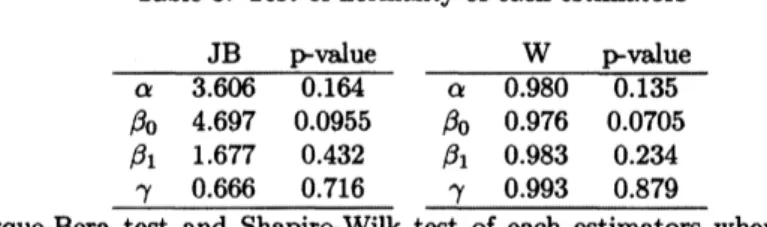
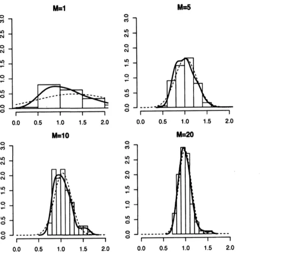
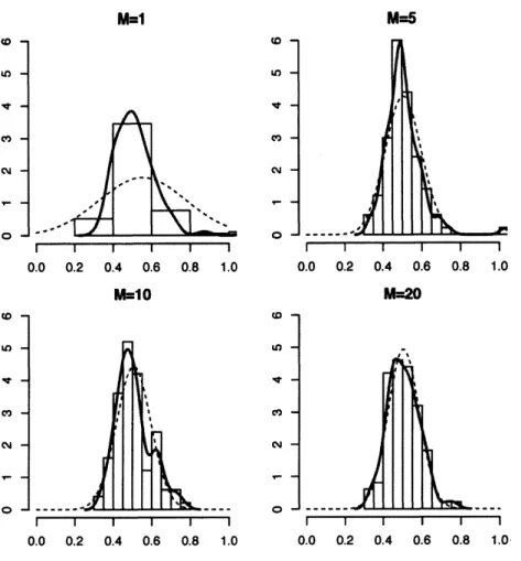
$l4om$_{figures 1, 2, 3and 4, the asymptotic normality startsto take holdfor allthe paxameterestimates}

as the number of markets increases where the additional moment condition is available. Thble 3.1 shows

that both Jarque-Bera andShapiro-Wilktestsdo notreject the normality hypothesisof the estimates with

$M=20,$ $R_{m}=100$and$T=1000.$

Whenwe canreasonably assume the asymptotic normality ofthe parameterestimates at $M=20$,

we

cantest whether the standarderrorofaestimatorwith$T=1000$issignificantlysmaller than that without

additionalmoments. Table4shows the resultofthe test. From theresult,accuracyimprovingeffectsof the

Table 1: MonteCarlo Simulation Resultsof$(\alpha, \beta_{0})$ for MultipleMarketsModel With/WithoutAdditional Moment 1(K)repetitions, withnosamplingerror $\langle J=20,$ $n=10,$$0\infty,$ $n_{m}=n/M,R_{m}=100$each)

$\#$of $\alpha(1.0)$ $\#$of $\beta_{\mathfrak{o}}(1.0)$

Consumer $\#$ofMarkets(M) Consumer $\#$ofMarkets (M)

$\frac{Draw\epsilon(T)151020Draws(T\rangle 151020}{001.269941.033131.016450.975081.528521.073611.039040.95\mathfrak{M}}$

(1.03294) (0.37532) (0.204981) (O.158212) $\langle$1.86754$)$ (0.690521) $(0.36\infty 34)$ (0.283556)

1.31111 1.06338 1.04777 1.00239 1.57892 1.13397 1.09765 1.01297

se

so

(0.875849) (0.374163) (0.256261) (0.214051) (1.00783) (0.681033) (0.454746) (0.371711) 1.31559 1.0212 1.03771 0.984661 1.59892 1.05349 1.07691 0.98192 $1\infty$ 100 (0.867226) $(0.2\Re KP3)$ (0.273552) (0.206735) (1.59301) (0.530612) (0.492299) (0.368529) 1.31444 1.02442 1.04496 0.991862 1.58161 1.0548 1.08701 0.987647 $5\infty$ 500

(0.825948) $(0.2\mathfrak{V}638)$ (O.191984) (O.141564) (1.517) (0.455524) (0.353673) (0.257662)

1.29778 1.03497 1.0447 0.999625 1.54479 1.07235 1.08683 0.999648

$1\propto K\}$ $1\alpha n$

(0.823522) (0.247841) (O.191337) $(0$.128913$)$ (1.51631) (0.464049) (0.354719) (0.237586)

%ble_{2: Monte Carlo Simulation} $R\epsilon$sults of$(\beta_{1}, \gamma)$ for MultipleMarkets Model_$With/$Without

Additional Moment

$\overline{\#}$

of

$\beta_{1}(0.5)100$

repetitions, with no

$smpling\#of$error $(J=20, n=10,000, n_{n}\gamma(1.5\rangle=n/M,R_{m}=100$each)

Consumer $\#$of Markets(M) $co1\mathfrak{B}$umer $\#$ofMarkets(M)

$\frac{Draws(T)1510\mathfrak{A})Draws(T)151020}{000.566090.4923\Re 0.5242970.5145951.448681.476121.487031.47739}$

(0.679877) (O.237166) $\langle$O.172493$)$ (O.10943\^o) (0.239105) (0.113698) _{$(0.0793864\rangle$} ($0$.OS60014)

0.580772 0.522223 0.523877 0.522409 i.49485 1.48419 1.49174 1.$4788S$

se

50

(O.SS5857) (O.21608) $(0.209301\rangle$ $(0.212403\rangle$ $(0.2\propto)528\rangle$ (0.126429) (0.0952291) $\langle$0.0929717$)$

0.593833 0.53132 0.530457 0.533023 1.49347 1.47787 1.49048 1.47432

$100 1\alpha)$

(0.32299) (O.I60593) (0.162806) $($O.$163413\rangle$ $(0.222(\}92\rangle$ (O.$108769\rangle$ (0.0816977) (0.0846689)

$0.554(\hslash 7$ 0.505637 _O.W5657 0.504008 _{1.50725 1.48927 1.50225 1.48696}

mo

500

$(0.224106\rangle$ _{$(0.093237\rangle (0.0901611) (0.0807463) \langle O.198426)$ $(0.0\Re\}8213)$ (0.0655352) (0.0587172)}

0.565112 0.496941 0.506038 $0.494\}23$ _{1.49857 1.4931} $1.\alpha\}303$ 1.49161

$10\infty 1\alpha n$

$(0_{\backslash }239662)$ (0.0702588) (0.0696279) (0.0609522) $(O.2\propto k2)$ (0.0898322) (0.0625012) (0.0542441)

Table

3:

Test ofnormalityof each estimators

$\frac{JBp-va1ue}{\alpha 3.6060.164} \frac{Wp-va1ue}{\alpha 0.9800.135}$

$\beta_{0}$ 4.697 0.0955 $\beta_{0}$ 0.976 0.0705 $\beta_{1}$ 1.677 0.432 $\beta_{1}$ 0.983 0.234

$\gamma$ 0.666 0.716 $\gamma$ 0.993 0.879

Jarque-Bera test and Shapiro-Wilk test of each estimators when $M=$

$20,$$T=1000$and $R_{w}=100.$

Table4: Testofvariancesof theestimators

$\frac{F-.vduep-vduedf}{\alpha 150620.0214(99,99)}$

$\beta_{0}$ 1.4244 0.03998 $(99,99)$ $\beta_{1}$ 3.2236 7.$80E-09$ $(99,99)$

$\gamma$ 1.4985 0.02274 $(99,99)$

Alternative hypothesis: thevarianceoftheestimator when$M=20,$$T=0$

is greater than that when$M=20,$ $T=1000$

4

Conclusion and

Discussion

Inthis paper, weimplement MonteCarlo simulation to examineasymptotic propertiesof the estimator of

random-coefficient logitmodels ofdemandfor non-durableconsumergoods underanequilibrium assumption

in thepresenceofmicro moments

as

the number of the examined regionalmarketsincreases. Thenational

micro moments

are

manufactured from the joint distribution of demographic information of

consumers

choosing those products with certain discriminating attributes. We observe that adding

an

equilibrium assumptionand themicromomentsgives asymptotic normality with sharper asymptoticvariance-covariance

matrix,while correctingasymptoticbiasreportedinReyberger (2015),anunexpected and rather surprising result.

Expandingthenumber ofmarkets toexamine

seems

agoodidea atfirst, becauseit simplyincreasesthe

number of

consumers

to be analyzed. Our Monte Carloexperiments

as

well

as

that ofFreyberger (2015)

show thatthisis not necessarily so, because thereisno mechanism inherentinthisincrease inthenumber of

marketsto guarantee that the samplingisdone randomlyand doingso enables to achieveagood coverage

of the nationalmarket. It

seems

adding “national” micro momentswillcorrectpossiblebiasinherent inthis

increase inthe number of markets. Furtherresearchis needed to understandthe mechanism under which

References

[1] Berry, S., “Estimating Discrete-Choice Models of Product Di{ferentiation,’’ RAND Journal

_of

Eco-nomics, 25 (1994), 242-262.

[2J Berry, S., J. Levinsohn, and A. Pakes, “AutomobilePrices in MarketEquilibrium Econometrica, 63

(1995),841-890.

[3] Berry, S.,J. Levinsohn, andA.Pakes, “DifferentiatedProducts DemandSystems fromaCombination

ofMieroandMacro_{Data: The New Car Market,“ Journal}

_of

_{PoliticalEconomy, 112 (2004),}

_69-105.

[4] Berry, S.,O. Linton, andA. $\ddagger>$akes,

“Limit Theorems for Estimating the Parameters of Differentiated

Product Demand Systems Review

_of

Economic Studies, 71 (2004), 613-654.

[5] ConsumerExpenditures and income, The US BureauofLabor Statistics, April,2007.

[6] Bresnahan, J., “EmpiricalStudiesofIndustrieswithMarket Power Handbook

_of

industrial$0\eta aniza-$

tion, $ed$, byR. Schmalensee, and R. WStlig, _{vol. 2.} $(1989\rangle$,North-Holland.

$|7]$ Freyberger, J., (Asymptotic theory for diffbrentiated

products demand models wlth many markets,”

Journal

_of

Econometrics, 185 (2015), 162-181.

[8] Imbens, G. and T. Lancaster, “Combining Micro and Macro DatainMicroeconometricModels Review

of

EconomicStudies, 61 (1994), 666-680.

[9] Myojo, S. and Kanazawa, Y., “On Asymptotic Properties ofthe Parameters of Differentiated

Prod-uct Demand _{and Supply Systems When Demographically-Categorized Purchasing Pattern Data}

_are

Available International EconomicReview, 53(3) (2012),

887-938.

$|10]$ Nevo,A., “Measuring Market Power in_{the Ready-t}$(\succ Eat$ _{CerealIndustry,}$”$

Econometrica, $69 (2001)$_,

307-342.

[11] Pakes, A., ”

Patents as Options: Some Estimatesofthe Valueof Holding European Patent Stocks, ”

Econometrica, 54$\langle$1986),

765-784.

[12] Petrin,_{A., “Quantifying the Benefits of New Products: The Case of theMinivan Journal}

_of

_Political Economy, 110 (2002), 705-729.

[13] $Sudhir_{\rangle}$ K., “Competitive Pricing Behavior in the Auto Market: A

Structural Analysis,“ Marketing

M$=$$ M#

$O \overline{III||}$

0.0 0.5 t.O 1.5 2.0 0.0 0.5 t.O 1.5 2.0

$M=10$

0.0 0.5 7.0 I.5 20 0.0 0.51.0 1.5 2.0

Figure 1: Histograms for the $\alpha$with theadditional moment $(T=500)$ with thenumber $M=1,$

$S$,10,20of

markets. Densityestimates(solid)

as

wellasthe normal

curves

(dashed)forthe$\alpha$with the estimated

mean

$M=1$ $MS-$

o.o

0.$5$ 1.$0$ 7.$5$ 2.$0$ 2.5

o.o

$0.s$ _1.$0$ 1.$5$ 2.$0$ 2.5

$M=10 M=20$

0.$0$ 0.5 _$.O 1.5 2.0

2.5 0.$0$ 0.$5$ 1.0 _$.5 2.0 2.5

Figure 2: Histogram of $\beta_{0}$ with additional micro moment $(T=500)$ with the number $M=1$, 5,10,

20 of

markets. Densityestimates (solid)

as

well

as

the normal

curves

(dashed) for the$\beta_{0}$withtheestimatedmean

kl $MS-$

0.$0$ 0.$2$ 0.$4$ 0.$6$ 0.8 t.O 0.0 0.2 0.4 0.6 0.8 1.0

k10 $M=20$

0.0 0.2 0.4 0.6 O.S 1.0 0.0 0.2 0.4 0.6 O.S 1.0

Figure 3: Histogram of $\beta_{1}$ with the additional moment $(T=500)$ with the number $M=1$ , 5, 10,20 of

markets. Densityestimates(solid)aswellasthe normalcurves(dashed) for the$\beta_{1}$ with the estimatedmean

$M=S$ $M\simeq S$

S.O t.2 1.4 1.6 3.8 2.0 10 1.2 7.4 1.6 1.8 2.0

$M=10$

1.0 1.2 IA 1.6 2.8 2.$O$ t.O 1.2 t4 1.6 7.8

ao

Figure4; _Histogramof$\gamma$withthe additional moment $(^{r}f=500$) withthe number$M=1$,5, 10,20of markets.

Density estimates (solid) as well as the normal curves $\langle$dashed) for the

$\gamma$ with the estimated

mean

and