Global structure of plane closed elastic curves (New developments of the theory of evolution equations in the analysis of non-equilibria)

Global

structure

of

plane

closed elastic

curves

Murai Minoru(Ryukoku University)

1

Introduction

This is

a

joint work with Waichiro Matsumoto and Shoji Yotsutani

(Ryukoku University).

Let$\Gamma$ beapl$\mathfrak{W}1e$closed elastic

curve

with length $2\pi$

.

We denotearc-length

and curvature by $s$ and $\kappa(s)$, respectively. Let $M$ be the signed

area

defined

by

$M:= \frac{1}{2}\int_{\Gamma}xdy-ydx,$

where $(x, y)=(x(s), y(s))\in\Gamma$ with $(x(O), y(O))$ $:=(0,0)$

.

Let

us

consider the

following variational problem $(VP)$:

Find

a curve

$\Gamma$ (the curvature $\kappa(s)$) which minimize $\frac{1}{2}\int_{0}^{2\pi}\kappa(s)^{2}ds$

subject to $\pi>M$ _and $\omega\pi\neq M$, where $\omega$ is the winding number.

K.

Watanabe

([1, 2])

considered

this

variational

problem $(VP)$ with $\omega=$

$1$

.

He derived the Euler-Lagrange equation to $(VP)$ and showed the existence

of the minimizer arid investigate the profile near the disk.

The Euler-Lagrange equation to $(VP)$ is

$(P^{\omega})\{\begin{array}{l}\kappa_{ss}+\frac{1}{2}\kappa^{3}+\mu\kappa-\nu=0, s\in[0,2\pi],\kappa(0)=\kappa(2\pi), \kappa_{s}(0)=\kappa_{s}(2\pi) ,\frac{1}{2\pi}\int_{0}^{2\pi}\kappa(s)ds=\omega,4\mu\pi^{2}+\pi\int_{0}^{2\pi}\kappa(s)^{2}ds\overline{4\pi\omega\mu+\int_{0}^{2\pi}\kappa(s)^{3}ds}=M,\end{array}$

where $\mu$ and $\nu$

are some

constants. We can obtain the following proposition

by using the argument of K.Watanabe [1, Lemma 3 and Lemma 4]

Proposition 1.1 Suppose that $\kappa(s)$ is a solution

of

$(P^{\omega})$, then the following

properties hold:

(i) $\kappa(s)\in C^{\infty}([0,2\pi])$

.

with period $\mathcal{S}=2\pi/m$ and axially symmetric with respect to _$s=\pi/m$ and

$m$ denotes the number

of

minimum points

of

$\kappa(s)$ by normalizing $\kappa(0)$ $:=$

$\max_{0\leq s\leq 2\pi}\kappa(s)$

.

(We call this solution $tm$ –mode $\mathcal{S}$olution

”

$.$)

Let us normalize $\kappa(s)$

as

$\kappa(0)$ $:= \max_{0\leq s\leq 2\pi}\kappa(s)$

.

For $n$-mode solution $\kappa(\mathcal{S})$, we may consider the following differential equation:

$(P_{n}^{\omega})\{\begin{array}{ll}\kappa_{ss}+\frac{1}{2}\kappa^{3}+\mu\kappa-\nu=0, s\in[0, \frac{\pi}{n}], (1.1)\kappa_{S}(0)=\kappa_{s}(\frac{\pi}{n})=0, \kappa_{s}(s)<0s\in(0, \frac{\pi}{n}), (1.2)\int_{0}^{\pi/n}\kappa(s)d_{\mathcal{S}}=\frac{\omega\pi}{n}, (1.3)\frac{2\mu\pi^{2}+n\pi\int_{0}^{\pi/n)}\kappa(s)^{2}ds}{2\pi\omega\mu+n\int_{0}^{\pi/n}\kappa(s)^{3}ds}=M. (1.4)\end{array}$

We introduce the followingauxiliary problem. Let $\kappa(s)$ be unknown

func-tion, and $\mu,$ $\nu$ be unknown constants. Find _{$(\kappa(s), \mu, \nu)$} such that

$(E_{n})\{\begin{array}{ll}\kappa_{SS}+\frac{1}{2}\kappa^{3}+\mu\kappa-\nu=0, s\in[0, \frac{\pi}{n}], (1.5)\kappa_{s}(0)=\kappa_{s}(\frac{\pi}{n})=0, \kappa_{s}(s)<0 for s\in(0, \frac{\pi}{n}) .(1.6)\end{array}$

First we represent all solution $(\kappa(s), \mu, \nu)$ of $(E_{n})$. Next

we

give the

representation of the constraint (1.3) and (1.4).

We prepare notations to state

our

theorems.

Definition 1.1 We

_define

the complete elliptic integral

_of

first, second and

third kind by

$K(k) ;= \int_{0}^{1}\frac{d\xi}{\sqrt{(1-\xi^{2})(1-k^{2}\xi^{2})}},$

$E(k) ;= \int_{0}^{1}\sqrt{\frac{1-k^{2}\xi^{2}}{1-\xi^{2}}}d\xi,$

Definition 1.2

Jacobi’s

sn

_function

is

_defined

by

$z= \int_{0}^{sn(z,k)} d\xi$

$\sqrt{(1-\xi^{2})(1-k^{2}\xi^{2})}$

and Jacobi’s cn

_function

is

_defined

by

$cn(z, k):=\sqrt{1-sn^{2}(z,k)}$

for

$z\in[-K(k), K(k)]$

.

These elliptic

functions

are

extended

to $(-\infty, \infty)$

by using the relation

sn

$(z+2K(k), k)=-$

sn

$(z, k)$ and

cn

$(z+2K(k), k)=$

$-cn(z, k)$

.

1.1

Main Result

Theorem 1.1 All solutions $(\kappa(s), \mu, v)$

of

$(E_{n})$

are

represented by the

fol-lowing (i), (ii) and (iii):

(i) $\kappa(s)=\overline{\kappa}_{n}(s;k, h),$ $\mu=\overline{\mu}_{n}(k, h)$ and $\nu=\overline{\nu}_{n}(k, h)$

for

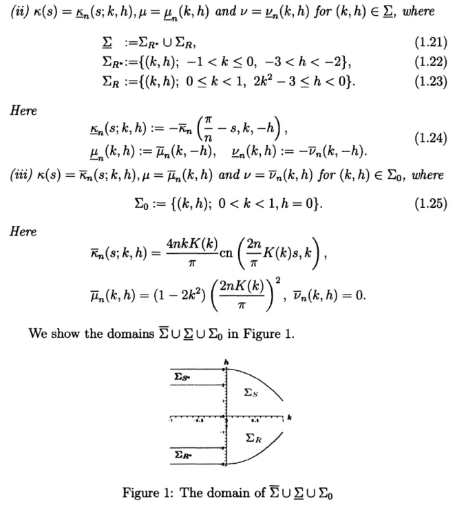
$(k, h)\in\overline{\Sigma}$, where

$\overline{\Sigma} :=\Sigma_{S^{*}}\cup\Sigma_{S}$, (1.7)

$\Sigma_{S^{*}};=\{(k, h);-1<k\leq 0,2<h<3\}$, (1.8) $\Sigma_{S}:=\{(k, h);0\leq k<1,0<h\leq 3-2k^{2}\}$, (1.9)

$\overline{\kappa}_{n}(\mathcal{S};k, h):=\{\begin{array}{l}\kappa_{n}^{s*}(s;k, v(k, h)) for (k, h)\in\Sigma_{S^{*}},\kappa_{n}^{S}(s;k, u(k, h)) for (k, h)\in\Sigma_{S},\end{array}$ (1.10)

$\overline{\mu}_{n}(k, h)$ $;=\{\begin{array}{ll}\mu_{n}^{s*}(k, v(k, h)) for (k, h)\in\Sigma_{S^{*}},\mu_{n}^{s}(k, u(k, h)) for (k, h)\in\Sigma_{S},\end{array}$ (1.11)

and

$\overline{\nu}_{n}(k, h):=\{\begin{array}{l}\nu_{n}^{S^{*}}(k, v(k, h)) for (k, h)\in\Sigma_{S^{*}},\nu_{n}^{\mathcal{S}}(k, u(k, h)) for (k, h)\in\Sigma_{S}.\end{array}$ (1.12)

Here the

_functions

$\kappa_{n}^{*}(s;k, v),$ $\mu_{n}^{*}(k, v),$ $\nu_{n}^{*}(k, v)$ and$v(k, h)$ are

defined

by

$\kappa_{n}^{S^{*}}(s;k, v):=-\frac{\sqrt{1-v}\sqrt{(1-k^{2})v+1+k^{2}}}{\sqrt{v+1}(2-(1+v)cn^{2}(\frac{n}{\pi}K(k)(\frac{\pi}{n}-s),k))}(\frac{4\sqrt{2}n}{\pi}K(k))$

(1.13)

$\mu_{n}^{S^{*}}(k, v);=(\frac{-3(4-(1-k^{2})(1-v)^{2})^{2}}{(1-v^{2})((1-k^{2})v+1+k^{2})}+8(2-k^{2}))(\frac{n}{2\pi}K(k))^{2}$ (1.14) $\nu_{n}^{S^{*}}(k, v);=\frac{-2\sqrt{2}(4-(1-k^{2})(1-v)^{2})}{(1-v^{2})^{3/2}((1-k^{2})v+1+k^{2})^{3/2}}.$ $((1+v)^{2}((1-k^{2})v+1+k^{2})^{2}-k^{4}(1-v)^{2}))( \frac{n}{2\pi}K(k))^{3}$ (1.15) and $v(k, h)$ $:= \frac{-2+(2-k^{2})(2-h)+\sqrt{(2-k^{2})^{2}(2-h)^{2}+4k^{4}(3-h)}}{2(1-k^{2})}$ (1.16)

and the

_functions

$\kappa_{n}(s;k, u),$$\mu_{n}(k, u),$ $v_{n}(k, u)$ and$u(k, h)$ are also

defined

by

$\kappa_{n}^{S}(s;k, u):=-\frac{(1-k^{2})(1-ku)+k((1-k^{2})u+k)cn(\frac{2n}{\pi}K(k)(\frac{\pi}{n}-s),k)}{(1-k^{2})u+k-k(1-ku)cn(\frac{2n}{\pi}K(k)(\frac{\pi}{n}-s)s,k)}.$ $\frac{\sqrt{u}\sqrt{(1-2k^{2})u+2k}}{\sqrt{(1-k^{2})u^{2}+1}}. (\frac{4nK(k)}{\pi})$ $+ \frac{(1-ku)((1-k^{2})u+k)}{\sqrt{u}\sqrt{(1-2k^{2})u+2k}\sqrt{(1-k^{2})u^{2}+1}}(\frac{2nK(k)}{\pi})$, (1.17) $\mu_{n}^{S}(k, u);=(\frac{-3(1-ku)^{2}((1-k^{2})u+k)^{2}}{2u((1-2k^{2})u+2k)((1-k^{2})u^{2}+1)}+1-2k^{2})$ (1.18) $( \frac{2nK(k)}{\pi})^{2}$ $v_{n}^{S}(k, u);= \frac{-(1-ku)((1-k^{2})u+k)}{4u^{3/2}((1-2k^{2})u+2k)^{3/2}((1-k^{2})u^{2}+1)^{3/2}}.$ $(4k^{2}((1-k^{2})u^{2}+1)^{2}+(1-k^{2})u^{2}((1-2k^{2})u+2k)^{2})$

.

(1.19) $( \frac{2nK(k)}{\pi})^{3}$ and $u(k, h);= \frac{1}{4k(1-k^{2})}\cdot(2-h+$ $\frac{(1-2k^{2})((2-h)^{2}+16k^{2}(1-k^{2}))}{8k^{2}(1-k^{2})+\sqrt{(1-2k^{2})^{2}(2-h)^{2}+16k^{2}(1-k^{2})}})$ (1.20)

$(i_{j}i)\kappa(s)=\underline{\kappa}_{n}(s;k, h),\mu=\underline{\mu}_{n}(k, h)$ and $v=\underline{\nu}_{n}(k, h)$

for

$(k, h)\in\underline{\Sigma}$, where

$\underline{\Sigma} :=\Sigma_{R^{*}}\cup\Sigma_{R}$, (1.21)

$\Sigma_{R}\cdot;=\{(k, h);-1<k\leq 0, -3<h<-2\}$, (1.22) $\Sigma_{R}:=\{(k, h);0\leq k<1,2k^{2}-3\leq h<0\}$

.

(1.23)

Here

$\underline{\kappa}_{n}(s;k, h):=-\overline{\kappa}_{n}(\frac{\pi}{n}-s, k, -h)$ ,

(1.24)

$\underline{\mu}_{n}(k, h) :=\overline{\mu}_{n}(k, -h) , \underline{\nu}_{n}(k, h) :=-\overline{\nu}_{n}(k, -h)$

.

(iii) $\kappa(s)=\overline{\kappa}_{n}(s;k, h),\mu=\overline{\mu}_{n}(k, h)$ and $\nu=\overline{\nu}_{n}(k, h)$

for

$(k, h)\in\Sigma_{0}$, where $\Sigma_{0};=\{(k, h);0<k<1, h=0\}$

.

(1.25)

Here

$\overline{\kappa}_{n}(s;k, h)=\frac{4nkK(k)}{\pi}cn(\frac{2n}{\pi}K(k)s, k)$ ,

$\overline{\mu}_{n}(k, h)=(1-2k^{2})(\frac{2nK(k)}{\pi})^{2}, \overline{v}_{n}(k, h)=0.$

We show the domains $\overline{\Sigma}\cup\underline{\Sigma}\cup\Sigma_{0}$ in Figure 1.

Figure 1: The domain of$\overline{\Sigma}\cup\underline{\Sigma}\cup\Sigma_{0}$

Remark 1.1 It is

more

_useful

by using the parameter $(k, u)$ and $(k, v)$ than

$(k, h)$

.

Let

us

set

$\Sigma_{v};=\{(k, v);-1<k\leq 0, -1<v<1/k\}$, (1.26)

$\Sigma_{u};=\{(k, u);0<k<1,0<u<1/k\}$

.

(1.27)

Then thefolloutng (i), (ii),(iii) and (iv) hold:

(i) Changing the parameters

_from

$(k, h)$ to $(k, v)$ by $k=k$ and $v=v(k, h)$,

(ii) Changing the parameter

_from

$(k, h)$ to $(k, u)$ by $k=k$ and $u=u(k, h)$,

$\Sigma_{S}become\mathcal{S}\Sigma_{u}.$

(iii) Changing the pammeter

_from

$(k, h)$ to $(k, u)$ by $k=k$ and$u=u(k, -h)$,

$\Sigma_{R}$ becomes $\Sigma_{u}.$

(iv) Changing the pammeter

_from

$(k, h)$ to $(k, v)$ by $k=k$ and$v=v(k, -h)$,

$\Sigma_{R^{*}}$ becomes $\Sigma_{v}.$

We note that all changing the pammeters

are

bijective.

We show the domains $\Sigma_{v}$ arid $\Sigma_{u}$ in Figure 2.

Figure 2: The domains $\Sigma_{v}$ and $\Sigma_{u}$

Theorem 1.2 Let $\kappa(s)$ be given by Theorem 1.1 and

$Z(k, h);= \int_{0}^{\pi/n}\kappa(s)ds.$

Then $Z(k, h)$ is given by the following $(i)_{f}(ii)$ and (iii):

(i) $Z(k, h)=\overline{Z}(k, h)for(k, h)\in\overline{\Sigma}$, where

$\overline{Z}(k, h):=\{\begin{array}{l}Z^{S^{*}}(k, v(k, h)) for (k, h)\in\Sigma_{S^{*}},Z^{S}(k, u(k, h)) for (k, h)\in\Sigma_{S}.\end{array}$

Here the

_function

$Z^{S^{*}}(k, v)\iota s$

defined

by

$Z^{S^{*}}(k, v):= \frac{Z_{\infty}^{*}(k,v)}{Z_{0}^{*}(k,v)}$, (1.28)

$Z_{\infty}^{*}(k, v):=((1-k^{2})(1+v)(3-v)+4k^{2}v)K(k)$ (1.29) $-4(1-k^{2})(1-v^{2}) \Pi(\frac{1}{2}(1-k^{2})(1-v)-1, k)$ ,

and the

_function

$Z^{s}(k, u)$ is also

defined

by $Z^{s}(k, u):= \frac{2((1-k^{2})u+k)Z_{\infty}(k,u)}{Z_{0}(k,u)}$, (1.31) $Z_{\infty}(k, u):=(2(1-k^{2})u^{2}+2-(1-ku)^{2})K(k)$ (1.32) $-2((1-k^{2})u^{2}+1) \Pi(\frac{k^{2}(1-ku)^{2}}{u((1-2k^{2})u+2k)}, k)$ , $Z_{0}(k, u)$ $:=(1-ku)\sqrt{u}\sqrt{(1-2k^{2})u+2k}\sqrt{(1-k^{2})u^{2}+1}$

.

(1.33) (1.34) (ii) $Z(k, h)=\underline{Z}(k, h)$

for

$(k, h)\in\underline{\Sigma}$, where

$\underline{Z}(k, h) :=-\overline{Z}(k, -h)$

.

(iii) $Z(k, h)=0$

for

$(k, h)\in\Sigma_{0}.$

The relation $Z(k, h)$ is represented by twoforms$\overline{Z}(k, h)$ and$\underline{Z}(k, h)$

.

The

$curvesofZ(k, h)=$ inthecase $\omega=0$ inFigure 3

$relationZ(k, h)=\frac{\omega\pi}{n,0}isequiva1$entto ($1.3).$ Forexample,

we

show the level

Figure 3: The level

curves

of $Z(k, h)=0$

Theorem 1.3 Let $\kappa(s)$ be given by Theorem 1.1 and

Then $\mathcal{E}_{n}(k, h)$ is given by the following (i), (ii) and (iii):

(i) $\mathcal{E}_{n}(k, h)=\overline{\mathcal{E}}_{n}(k, h)$

for

$(k, h)\in\overline{\Sigma}$, where

$\overline{\mathcal{E}}_{n}(k, h):=\{\begin{array}{l}\mathcal{E}_{n}^{s*}(k, v(k, h)) for (k, h)\in\Sigma_{S^{*}},\mathcal{E}_{n}^{s}(k, u(k, h)) for (k, h)\in\Sigma_{S}.\end{array}$ (1.35)

Here the

_function

$\mathcal{E}_{n}^{s*}(k, v)$ is

defined

by

$\mathcal{E}_{n}^{s*}(k, v):=\frac{2n^{2}}{\pi}K(k)$.

$(( \frac{(4-(1-k^{2})(1-v)^{2})^{2}}{(1-v^{2})((1-k^{2})v+k^{2}+1)}+8k^{2}-16)K(k)+16E(k))$

(1.36)

and the

_function

$\mathcal{E}_{n}^{S}(k, u)$ is also

defined

by

$\mathcal{E}_{n}^{S}(k, u):=\frac{4n^{2}}{\pi}K(k)$

.

$( \frac{(1-ku)^{2}((1-k^{2})u+k)^{2}K(k)}{u((1-2k^{2})u+2k)((1-k^{2})u^{2}+1)}-4((1-k^{2})K(k)-E(k)))$

.

(1.37)

(ii) $\mathcal{E}_{n}(k, h)=\underline{\mathcal{E}}_{n}(k, h)$

for

$(k, h)\in\underline{\Sigma}$, where

$\underline{\mathcal{E}}_{n}(k, h):=\overline{\mathcal{E}}_{n}(k, -h)$

.

(iii) $\mathcal{E}_{n}(k, h)=\overline{\mathcal{E}}_{n}(k, h)$

for

_{$(k, h)\in\Sigma_{0}$}, where

$\overline{\mathcal{E}}_{n}(k, h)=\frac{-16n^{2}}{\pi}K(k)\cdot((1-k^{2})K(k)-E(k))$

.

Theorem 1.4 Let $(\kappa(s), \mu, \nu)$ be given by Theorem 1.1 with (1.3) and $h\neq 0$

and

$M_{n}(k, h):= \frac{2\mu\pi^{2}+n\pi\int_{0}^{\pi/n)}\kappa(s)^{2}ds}{2\pi\omega\mu+n\int_{0}^{\pi/n}\kappa(s)^{3}ds}.$

Then $M_{n}(k, h)$ is given by the following (i) and (ii):

(i) $M_{n}(k, h)=\overline{M}_{n}(k, h)$

for

$(k, h)\in\overline{\Sigma}$, where

Here the

_function

$M_{n}^{s*}(k, v)$ is

defined

by $\underline{M}_{n}^{s}.(k, v):=\frac{\sqrt{2}\pi^{2}}{n}\cdot\frac{\sqrt{1-v^{2}}\sqrt{(1-k^{2})v+k^{2}+1}}{((1-k)v+1+k)}\cdot\frac{\varphi_{1}(k,v)}{\varphi_{2}(k,v)}\cdot\frac{1}{K(k)^{2}},$ $(1.39)$ $\varphi_{1}(k, v)$ $:=(-(1-k^{2})(1-v)^{2}+4)^{2}K(k)$ (1.40) $-8(1-v^{2})((1-k^{2})v+k^{2}+1)E(k)$, $\varphi_{2}(k, v)$ $:=((1+k)v+1-k)((1-k^{2})(v+1)^{2}+4k^{2})$

.

(1.41) $(-(1-k^{2})(1-v)^{2}+4)$

and the

_function

$M_{n}^{S}(k, u)$ is also

defined

by

$M_{n}^{s}(k, u):= \frac{-\pi^{2}}{2n}\cdot\frac{\sqrt{u}\sqrt{(1-k^{2})u^{2}+1}\sqrt{(1-2k^{2})u+2k}}{(1-ku)((1-k^{2})u+k)}\cdot\frac{\varphi_{3}(k,u)}{\varphi_{4}(k,u)}\cdot\frac{1}{K(k)^{2}},$

(1.42)

$\varphi_{3}(k, u)$ $:=-((1-ku)^{2}((1-k^{2})u+k)^{2}$ (1.43)

$+u((1-2k^{2})u+2k)((1-k^{2})u^{2}+1))K(k)$ $+2u((1-2k^{2})u+2k)((1-k^{2})u^{2}+1)E(k)$,

$\varphi_{4}(k, u)$ $:=k^{2}(1-ku)^{2}((1-k^{2})u^{2}+1)$ (1.44)

$+u((1-2k^{2})u+2k)((1-k^{2})u+k)^{2}$

(ii) $M_{n}(k, h)=\underline{M}_{n}(k, h)$

for

$(k, h)\in\underline{\Sigma}_{f}$ where

$\underline{M}_{n}(k, h)=-\overline{M}_{n}(k, -h)$

.

For given $M$, the solutions of transcendental equations

$Z(k, h)= \frac{\omega\pi}{n}, M_{n}(k, h)=M$ (1.45)

give the solution of $(P_{n}^{\omega})$ by Theorem 1.1.

For example, let

us

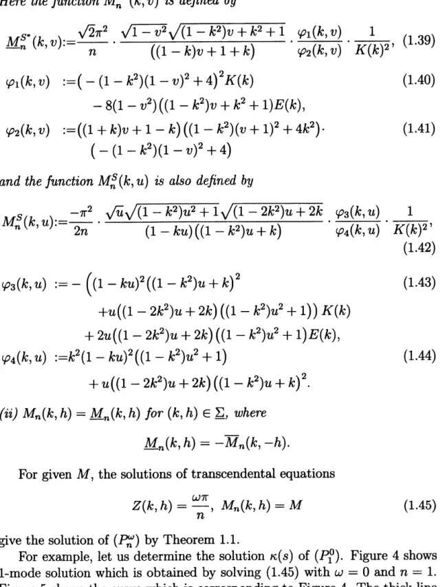
determine the solution $\kappa(s)$ of $(P_{1}^{0})$

.

Figure 4 shows

1-mode solution which is obtained by solving (1.45) with $\omega=0$ and $n=1.$

Figure 5 shows the

curve

which is corresponding to Figure 4. The thick-line

$hI=0.\Re’. M\triangleleft$ $M^{--}\triangleleft.\theta 9$

$r\Rightarrow 1.14$ $M$–2.26 $\mathfrak{U}\cdot\cdotarrow-\pi$

Figure 4: Curvatures of 1-mode solution for $\omega=0$

$\mapsto\pi raz\epsilon u_{-\backslash }l.14$

$M^{z}4.3y. u\triangleleft *\cdots O.\theta 9$

u–1.14 _r-r-2.ffl $I^{\ovalbox{\tt\small REJECT}}arrow-\pi$

Figure 5: Curves of 1-mode solution for $\omega=0$

We note that the other

curves

are not closed except for $k=k_{0}$ with $h=0$

in Theorem 1.1, where $k_{0}$ is the unique solution of

$2E(k)-K(k)=0(0<$

$C_{\sim}^{\backslash }f_{-\cdot\vee}\prime\backslash :_{\grave{L}^{-\mathfrak{i}}}$

maae

aes

$rs\infty$

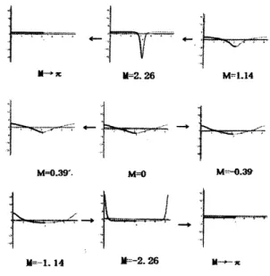
Figure 6: Energy

curves

ofstationary solutions for $\omega=0$

Figure 6 shows the energy

curves

of stationary solutions for $\omega=0$ which

are

obtained from the equation (1.45) and Theorem

1.3.

Investigating the global structure, we obtain the following theorems.

Theorem 1.5 Let $\omega=0$ and $n\geq 1$

.

Then, there exists

a

unique $n$-mode

solution $\kappa(s)=\kappa_{n}(s;M)$

of

$(P_{n}^{0})for- \frac{\pi}{n}<M<\frac{\pi}{n}.$ $\mathbb{R}$rther there exists

no

solution

_for

$M \leq-\frac{\pi}{n},$ $\frac{\pi}{n}\leq M.$

Theorem 1.6 Let$\omega=0$ and$n\geq 1$ Then, there exists

a

unique minimizer

$\kappa(s)=\kappa(s;M)for-\pi<M<\pi$ with the normalizing condition $\kappa(0)$ $:=$

$\max_{0\leq s\leq 2\pi}\kappa(\mathcal{S})$. This minimizer is 1-mode solution.

Theorem

1.7

Let $\omega=0$ and $n\geq 1$

.

Then, the $n$-mode solution $\kappa(s)=$

$\kappa_{n}(\mathcal{S};M)$

of

$(P_{n}^{0})$ with property $\kappa(0)$ _{$:= \max_{0\leq s\leq\pi/n}\kappa(s)$}

for

$0\leq s\leq\pi/n$

satisfies

the following relations:

(i) $\lim_{M\uparrow\frac{\pi}{n}}\kappa_{n}(s;M)=\{\begin{array}{ll}n for s\in[0, \frac{\pi}{n}) , uniformaly in [0, \frac{\pi}{n})-\infty f\alpha rs=\frac{\pi}{n}.\end{array}$

Inthis paper,

we

show theproofof Theorem 1.1. We need longcalculation

to obtain Theorem 1.$2\sim 1.7$

.

The complete proofs of them will appear in a

forthcoming papers.

This kind of method

was

first proposed by $Lou-Ni-Yotsut_{M1}i[5]$

.

Later,

Ikeda-Kondo-Okamoto-Yotsutani

[3] and Kosugi-Morita-Yotsutani [4]

devel-oped the method.

2

Proof

of Theorem 1.1

We rewrite $(E_{n})$ as first order differential equation to find the solution

$\kappa(s)$

.

Let

us

set

$\kappa(0):=\alpha, \kappa(\frac{L}{2n}):=\beta(\alpha>0, \alpha>\beta)$.

Multiplying $2\kappa_{S}$ to $(E_{n})$,

we

have

$\frac{d}{ds}(\frac{d\kappa}{ds})^{2}=\frac{d}{ds}(-\frac{1}{4}\kappa^{4}-\mu\kappa^{2}+2\nu\kappa)$

Integrating above equation on $[0, s]$, we obtain

$\frac{d\kappa}{ds}=-\sqrt{\tilde{g}(\kappa)}$, (2.1)

where

$\tilde{g}(\kappa)=-\frac{1}{4}\kappa^{4}-\mu\kappa^{2}+2\nu\kappa+\frac{1}{4}\alpha^{4}+\mu\alpha^{2}-2v\alpha$. (2.2)

By the Neumann boundary condition of $(E_{n})$,

we can

rewrite $\tilde{g}(\kappa)$

as

$\tilde{g}(\kappa)=\frac{1}{4}(\alpha-\kappa)(\kappa-\beta)((\kappa+\frac{\alpha+\beta}{2})^{2}+4\delta)$ , (2.3)

where $\delta$ is some

constarlt. Comparing the coefficients of (2.2) with that of

(2.3), we obtain

$\mu = \frac{-1}{8}(3(\alpha+\beta)^{2}-\frac{1}{2}(3\alpha+\beta)(\alpha+3\beta)-8\delta)$ ,

$\nu= \frac{1}{32}(\alpha+\beta)((\alpha-\beta)^{2}+16\delta)$

.

Let us set

Then $\mu$ and $\nu$

are

represented by

$\mu = \frac{-1}{8}(3(A+B)^{2}-8(AB+\delta))$,

(2.4)

$\nu= \frac{1}{8}(A+B)((A-B)^{2}+\delta)$

.

Further, let

us

set

$\hat{\kappa}:=\frac{1}{2}(\kappa+\frac{A+B}{2})$ (2.5) Then (2.1) is represented by $\frac{d\hat{\kappa}}{ds}=-\sqrt{\hat{g}(\hat{\kappa})},$ $\hat{\kappa}(0)=A,\hat{\kappa}(\frac{L}{2n})=B,$ (2.6) where $\hat{g}(\hat{\kappa})=(A-\hat{\kappa})(\hat{\kappa}-B)(\hat{\kappa}^{2}+\delta)$

.

(2.7)

We need to consider the following five

cases

in (2.6):

($i$) $A+B<0,$ $\delta\leq 0,$

(ii) $A+B<0,$ $\delta>0,$

(iii) $A+B>0,$ $\delta>0,$

(iv) $A+B>0,$ $\delta\leq 0,$

(v) $A+B=0.$

After the proofof Theorem 1.1, we obtain the following five equivalent

rela-tions:

($i$) $A+B<0,$ $\delta\leq 0\Leftrightarrow\Sigma_{S}\cdot,$

(ii) $A+B<0,$ $\delta>0\Leftrightarrow\Sigma_{S},$

(iii) $A+B>0,$ $\delta>0\Leftrightarrow\Sigma_{R},$

(iv) $A+B>0,$ $\delta\leq 0,$ $\Leftrightarrow\Sigma_{R}\cdot,$

($v$) $A+B=0,$$\delta\geq 0\Leftrightarrow\Sigma_{0},$

where $\Sigma_{S^{*}},$ $\Sigma_{S},$ $\Sigma_{R^{*}},$ $\Sigma_{R}$ arld $\Sigma_{0}$

are

given by (1.8), (1.9), (1.22), (1.23) and

(1.25), respectively.

We notethat there exists no solution for $A+B=0,$ $\delta<0$

.

We also note

that if $(\kappa(s),\mu, v)$ is a solution of $(E_{n})$, then $(-\kappa(\pi/n-s), \mu, -\nu)$ is also the

solution of $(E_{n})$ by (2.1) and (2.3). Hence if

we

have the solutions of $(E_{n})$ in

the

case

of (i) and (ii), then we also obtain the solutions of $(E_{n})$ in the

case

2.1

Representation of solutions for

$A+B<0,$

$\delta\leq 0$

Lemma 2.1 Suppose that $A+B<0$ and$\delta\leq 0$ in (2.6). Then the solution

$\kappa(s)$

of

$(E_{n})$ is represented by

$\kappa(s)=\kappa_{n}^{S^{*}}(s;A, B, \eta):=2\hat{\kappa}_{n}^{S^{*}}(s;A, B, \eta)-\frac{A+B}{2}+2\eta$, (2.8)

where $\eta$ $:=\sqrt{-\delta}$ and

$\hat{\kappa}_{n}^{S^{*}}(s;A, B, \eta):=\frac{(A-\eta)(B-\eta)}{B-\eta+(A-B)cn^{2}(\frac{n}{\pi}K(k)(\frac{\pi}{n}-s),k)}$. (2.9)

Moreover it holds that

$\sqrt{(A-\eta)(B+\eta)}=\frac{2n}{\pi}K(k)$ (2.10)

with

$k=-\sqrt{\frac{2\eta(A-B)}{(A-\eta)(B+\eta)}}$

.

(2.11)

Proof. Under the condition that $A+B<0$ and $\delta=-\eta^{2}\leq 0(\eta\geq 0)$, we

have

$B<A\leq-\eta\leq 0\leq\eta,$

since

$A>B$

and (2.7) is positive on the interval $(B, A)$. Now we show

$A\neq-\sqrt{-\delta}$

.

Assume that $A=-\sqrt{-\delta}<0$

.

Then, substituting $\hat{\kappa}=A-1/\xi$

into (2.6), we have $\frac{L}{2n}$ $=$ $\int_{B}^{A}\frac{d\hat{\kappa}}{(A-\hat{\kappa})\sqrt{-(\hat{\kappa}-B)(\hat{\kappa}+A)}}$ $= \frac{1}{\sqrt{-2A(A-B)}}\int_{1/(A-B)}^{\infty}\overline{\sqrt{(\xi-)(\xi-\frac{1}{2A})}}$ $= \frac{1}{\sqrt{-2A(A-B)}}[2\log|\sqrt{\xi-\frac{1}{A-B}}+\sqrt{\xi-\frac{1}{2A}}|]_{1/(A-B)}^{\infty}$ $=$ $\infty.$

This is

a

contradiction. In the

same

way,

we

obtain

in the

case

$A=-\sqrt{\eta}=0$

.

This is also contradiction. Thus it holds that $B<A<-\eta\leq 0\leq\eta$

.

(2.12) Let

us

set $\hat{\kappa}(s)=\frac{1}{\tilde{\kappa}(s)}+\eta$. (2.13) Then (2.6) becomes $\frac{d\tilde{\kappa}}{ds}=\sqrt{(A-\eta)(B-\eta)}\sqrt{(\tilde{\kappa}-\frac{1}{A-\eta})(\frac{1}{B-\eta}-\tilde{\kappa})(2\eta\tilde{\kappa}+1)}.$

Further

we

introduce change ofvariable $\tilde{\kappa}$

to $\varphi$ by

$\tilde{\kappa}(s)=\frac{1}{B-\eta}-(\frac{1}{B-\eta}-\frac{1}{A-\eta})\sin^{2}\varphi(s)$

for

$\varphi(s)\in[0,$ $\frac{\pi}{2}]$ (2.14) We obtain

$\frac{d\varphi}{ds}=\frac{-1}{2}\sqrt{(A-\eta)(B+\eta)}\sqrt{1-k^{2}\sin^{2}\varphi}.$

Integrating the above equation on $[0, s]$, we have

$\frac{\sqrt{(A-\eta)(B+\eta)}}{2}s=K(k)-\int_{0}^{\varphi(s)}\sqrt{1-k^{2}\sin^{2}\varphi’}d\varphi$ (2.15)

since $\varphi(0)=\pi/2$

.

At $s=\pi/n$, we obtain (2.10) by $\varphi(\pi/n)=0.$

Substituting (2. 10) and $\xi=\sin\varphi$ into (2. 15),

we

have

$\sin(\varphi(s))=$

sn

$( \frac{n}{\pi}K(k)(\frac{\pi}{n}-s),$$k)$ ,

which implies that

$\tilde{\kappa}(s)$ _$=$ $\frac{1}{A-\eta}+(\frac{1}{B-\eta}-\frac{1}{A-\eta})cn^{2}(\frac{n}{\pi}K(k)(\frac{\pi}{n}-\mathcal{S}),$$k)$

.

(2.16)

On the other hand, it follows from (2.5) and (2.13) that

we

have

$\kappa(s)=2\hat{\kappa}(s)-\frac{A+B}{2}=\frac{2}{\tilde{\kappa}(s)}-\frac{A+B}{2}+2\eta.$

2.2

_{Representation of solutions for}

_$A+B<0,$

$\delta>0$

Lemma 2.2 Suppose that $A+B<0,$$\delta>0$ in (2.6). Then the $\mathcal{S}$olution

of

$\kappa(s)$

of

$(E_{n})$ is represented by

$\kappa(s)=\kappa_{n}^{S}(s;A, B, \delta):=2\hat{\kappa}_{n}^{S}(s;A, B, \delta)-\frac{A+B}{2}$, (2.17)

where

$\hat{\kappa}_{n}^{S}(s;A, B, \delta):=$

$\frac{AB_{\delta}+A_{\delta}B-(AB_{\delta}-A_{\delta}B)cn(\frac{2n}{\pi}K(k)(\frac{\pi}{n}-s),k)}{A_{\delta}+B_{\delta}+(A_{\delta}-B_{\delta})cn(\frac{2n}{\pi}K(k)(\frac{\pi}{n}-s),k)}$, (2.18)

$A_{\delta}:=\sqrt{A^{2}+\delta}, B_{\delta}:=\sqrt{B^{2}+\delta}$_. (2.19)

Moreover it holds that

$\sqrt{A_{\delta}B_{\delta}}=\frac{2n}{\pi}K(k)$ (2.20)

with

$k= \sqrt{}\frac{1}{2}(1-\frac{AB+\delta}{A_{\delta}B_{\delta}})$

.

(2.21)

Proof.

Let us set

$\hat{\kappa}(s)=\frac{1}{\tilde{\kappa}(s)}+B$. (2.22)

Then (2.6) becomes

$\frac{d\tilde{\kappa}}{ds}=B_{\delta}\sqrt{A-B}\sqrt{(\tilde{\kappa}-\frac{1}{A-B})(\tilde{\kappa}^{2}+\frac{2B}{B_{\delta}^{2}}\tilde{\kappa}+\frac{1}{B_{\delta}^{2}})}.$

Further we introduce change of variable $\tilde{\kappa}$

to $\varphi$ by

$\tilde{\kappa}(s)=\frac{1}{A-B}(1+\frac{A_{\delta}}{B_{\delta}}\tan^{2}\frac{\varphi(s)}{2})$ , (2.23)

where $\varphi(\mathcal{S})\in[0, \pi]$

.

We get

$\frac{A_{\delta}}{(A-B)B_{\delta}}\tan\frac{\varphi}{2}(1+\tan^{2}\frac{\varphi}{2})\frac{d\varphi}{ds}$

$= \sqrt{A_{\delta}B_{\delta}}\cdot\frac{A_{\delta}}{(A-B)B_{\delta}}\tan\frac{\varphi}{2}\sqrt{1+\tan^{4}\frac{\varphi}{2}+2\frac{AB+\delta}{A_{\delta}B_{\delta}}\tan^{2}\frac{\varphi}{2}}$

$= \sqrt{A_{\delta}B_{\delta}}\cdot\frac{A_{\delta}}{(A-B)B_{\delta}}\cdot\tan\frac{\varphi}{2}\sqrt{(1+\tan^{2}\frac{\varphi}{2})^{2}-4k^{2}\tan^{2}\frac{\varphi}{2}}$

Thus

we

obtain

$\frac{d\varphi}{ds}=\sqrt{A_{\delta}B_{\delta}}\sqrt{1-k^{2}\sin^{2}\varphi}.$

Integrating the above equation on $[0, \mathcal{S}]$, we have

$\sqrt{A_{\delta}B_{\delta}}s=\int_{0}^{\varphi(s)} d\varphi$ (2.24)

$\sqrt{1-k^{2}\sin^{2}\varphi}$

by $\varphi(0)=0$. At $s=\pi/n$, we have (2.20) by $\varphi(\pi/n)=\pi.$

Substituting (2.20) and $\xi=\sin\varphi$ into (2.24),

we

obtain

$\sin\varphi(s)=$ sn $( \frac{2n}{\pi}K(k)s,$$k)$ ,

which implies that

$\cos(\varphi(s))=cn(\frac{2n}{\pi}K(k)s, k)$

Thus we have

$\tan^{2}\frac{\varphi(s)}{2}=\frac{1-\cos\varphi(s)}{1+\cos\varphi(s)}=\frac{1-cn(\frac{2n}{\pi}K(k)s,k)}{1+cn(\frac{2n}{\pi}K(k)s,k)}.$

Substituting above relation into (2.23), $\tilde{\kappa}(s)$ becomes

$\tilde{\kappa}(s) = \frac{A_{\delta}+B_{\delta}-(A_{\delta}-B_{\delta})cn(\frac{2n}{\pi}K(k)s,k)}{(A-B)B_{\delta}(1+cn(\frac{2n}{\pi}K(k)s,k))}$

.

(2.25)

On the other hand,

we

obtain

$\kappa(s)=2\hat{\kappa}(s)-\frac{A+B}{2}=2(\frac{1}{\tilde{\kappa}(s)}+B)-\frac{A+B}{2}$

by (2.5) and (2.22). Thus, substituting (2.25) into above relation, we obtain

(2.17) since

cn

$( \frac{2n}{\pi}K(k)s,$$k)=- cn(\frac{2n}{\pi}K(k)(\frac{\pi}{n}-s),$ $k)$

2.3

Change of parameters for

$A+B<0,$

$\delta\leq 0$

Let

us

consider the

case

$A+B<0,$$\delta\leq 0$. It is difficult for

us

to investigate

the global structure by using the parameters $A,$ $B$ and $\eta$ $:=\sqrt{-\delta}.$ $A$ and

$B$ belong to serm-infinite interval arld

$\eta$ is constrained by (2.20) and (2.21).

Thus

we

change the parameter.

Let

us see

$(k,\tilde{h})$ be known and _{$A,$ $B$} and

$\eta$ be the solutions of the system of

$\{\begin{array}{ll}k^{2}=\frac{2r\int(A-B)}{(A-\eta)(B+\eta)}, (2.26)\sqrt{(A-\eta)(B+\eta)}=\frac{2n}{\pi}K(k) , (2.27)A=(1-\tilde{h})B(0<\tilde{h}<2) .(2.28)\end{array}$

Then we obtain the following lemma:

Lemma 2.3 Suppose that

$A+B<0$

and $\delta\leq 0$

.

Then $A,$ $B$ and $\eta$

are

represented by

$A = - \frac{((1-k^{2})v+1)\sqrt{1-v}}{\sqrt{2}\sqrt{v+1}\sqrt{(1-k^{2})v+k^{2}+1}}\cdot(\frac{2n}{\pi}K(k))$,

$B = - \frac{(2-k^{2})v+k^{2}+2}{\sqrt{2}\sqrt{1-v^{2}}\sqrt{(1-k^{2})v+k^{2}+1}}\cdot(\frac{2n}{\pi}K(k))$, (2.29)

$\eta = \frac{k^{2}\sqrt{1-v}}{\sqrt{2}\sqrt{1+v}\sqrt{(1-k^{2})v+k^{2}+1}}. (\frac{2n}{\pi}K(k))$

and $v=v(k, h)$

for

$(k, h)\in\Sigma_{S^{*}}$, where $\Sigma_{S^{*}}$ and $v(k, h)$ are $def\dot{\ddagger}ned$ by (1.8)

and (1.16), respectively.

Proof.

It follows from (2.26),(2.27) and (2.28) that

we

obtain

$\eta=\frac{-k^{2}}{2\tilde{h}B}(\frac{2n}{\pi}K(k))^{2}$ (2.30)

Substituting (2.28) and (2.30) into (2.27), we have

$(1- \tilde{h})B^{4}-\frac{1}{2}(2-k^{2})(\frac{2n}{\pi}K(k))^{2}B^{2}-\frac{k^{4}}{4h^{2}}(\frac{2n}{\pi}K(k))^{4}=0.$

If $\tilde{h}\geq 1$, then the left hand

side of above equation is negative. Thus, we may

consider

$0<h<1$

. Solving the above equation with respect to $B$, we obtain

$A=-(1- \tilde{h})\xi(\frac{2n}{\pi}K(k)), B=-\xi(\frac{2n}{\pi}K(k))$ ,

(2.31)

since $B<0$, where

$\xi:=\frac{\sqrt{(2-k^{2})\tilde{h}+\sqrt{(2-k^{2})^{2}\tilde{h}^{2}+4k^{4}(1-\tilde{h})}}}{2\sqrt{\tilde{h}}\sqrt{1-\tilde{h}}}$

for

$(k,\tilde{h})\in\{(k,\tilde{h});0<k<1,0<\tilde{h}<1\}.$

To simplify the representation,

we

set

$v= \frac{-2+(2-k^{2})\tilde{h}+\sqrt{(2-k^{2})^{2}\tilde{h}^{2}+4k^{4}(1-\tilde{h})}}{2(1-k^{2})},$

which implies that

$2(1-k^{2})v+2-(2-k^{2})\tilde{h}=\sqrt{(2-k^{2})^{2}\tilde{h}^{2}+4k^{4}(1-\tilde{h})}$

.

(2.32)

Solving (2.32) with respect to $\tilde{h}$

yields

$\tilde{h}=\frac{(v+1)((1-k^{2})v+k^{2}+1)}{(2-k^{2})v+k^{2}+2}.$

Hence

we

have

$(2-k^{2})\tilde{h}+\sqrt{(2-k^{2})^{2}\tilde{h}^{2}+4k^{4}(1-\tilde{h})}=2(1-k^{2})v+2,$

$1- \tilde{h}=\frac{(1-v)((1-k^{2})v+1)}{(2-k^{2})v+k^{2}+2}$

by (2.32). Thus $\xi$ becomes

$\xi=\frac{(2-k^{2})v+k^{2}+2}{\sqrt{2}\sqrt{1-v^{2}}\sqrt{(1-k^{2})v+k^{2}+1}}.$

Substituting $h=\tilde{h}+2$ and above relation into (2.31), the lemma holds. $\square$

2.4

Change

of

parameters

for

$A+B<0,$

$\delta>0$

Let us consider the case $A+B<0,$$\delta>0$

.

It is also difficult for us to

investigate the global structure by using the parameters $A,$ $B$ and $\delta$

.

Thus

Let $(k,\tilde{h})$ be known and _{$A,$ $B$} and $\delta$ be the solutions of the system of

$\{\begin{array}{ll}k^{2}=\frac{1}{2}(1-\frac{AB+\delta}{\sqrt{(A^{2}+\delta)(B^{2}+\delta)}}) , (2.33)\sqrt[4]{(A^{2}+\delta)(B^{2}+\delta)}=\frac{2n}{\pi}K(k) , (2.34)A=(1-\tilde{h})B(0<\tilde{h}<2) .(2.35)\end{array}$

Then we obtain the following lemma:

Lemma 2.4 Suppose that $A+B<0,$ $\delta>0$

.

Then $A,$ $B$ and $\delta$

are

repre-sented by

$A = - \frac{\sqrt{u}(1-2k^{2}-2k(1-k^{2})u)}{\sqrt{(1-k^{2})u^{2}+1}\sqrt{(1-2k^{2})u+2k}}\cdot(\frac{2n}{\pi}K(k))$ ,

$B$ $=$ $- \frac{\sqrt{(1-2k^{2})u+2k}}{\sqrt{u}\sqrt{(1-k^{2})u^{2}+1}}\cdot(\frac{2n}{\pi}K(k))$ , (2.36)

$\delta= \frac{(1-k^{2})u((1-2k^{2})u+2k)}{(1-k^{2})u^{2}+1}. (\frac{2n}{\pi}K(k))^{2}$

and $u=u(k, h)$

for

$(k, h)\in\Sigma_{S}$, where _{$u(k, h)$} and $\Sigma_{S}$ are

defined

by (1.9)

and (1.20), respectively.

Proof. It follows from (2.34) and (2.33) that

we

obtain

$\delta=(1-2k^{2})(\frac{2n}{\pi}K(k))^{2}-(1-\tilde{h})B^{2}$

.

_(2.37)

Substituting (2.35) and (2.37) into (2.34), we have

$- \tilde{h}^{2}(1-\tilde{h})B^{4}+(1-2k^{2})\tilde{h}^{2}(\frac{2n}{\pi}K(k))^{2}B^{2}-4k^{2}(1-k^{2})(\frac{2n}{\pi}K(k))^{4}=0.$

Solving above equation with respect to $B$, we obtain the following two

solu-tions (i) and (ii):

(i)

$B= \frac{-2\sqrt{2}k\sqrt{1-k^{2}}}{\sqrt{\tilde{h}}\sqrt{(1-2k^{2})\tilde{h}+^{-}\sqrt{\tilde{h}^{2}-4k^{2}(1-k^{2})(2-\tilde{h})^{2}}}^{-}}.$

$( \frac{2n}{\pi}K(k))$

for

$(k,\tilde{h})\in\{(k,\tilde{h});0<k\leq 1/\sqrt{2}, H(k)<\tilde{h}<2\}$ $\cup\{(k,\tilde{h});1/\sqrt{2}<k\leq 1,1<\tilde{h}<2\},$

(ii)

$B= \frac{-2\sqrt{2}k\sqrt{1-k^{2}}}{\sqrt{\tilde{h}}\sqrt{(1-2k^{2})\tilde{h}-\overline{\sqrt{\tilde{h}^{2}-4k^{2}(1-k^{2})(2-\tilde{h})^{2}}}}}.$

$( \frac{2n}{\pi}K(k))$

since $B<0$, where

$H(k):= \frac{4k\sqrt{1-k^{2}}}{1+2k\sqrt{1-k^{2}}}.$

Further changing the parameter $(k,\tilde{h})$ to $(k, h)$ by

$h=\{\begin{array}{l}2-\sqrt{\tilde{h}^{2}-4k^{2}(1-k^{2})(2-\tilde{h})^{2}} for case (i),2+\sqrt{\tilde{h}^{2}-4k^{2}(1-k^{2})(2-\tilde{h})^{2}} for case (ii),\end{array}$

$\tilde{h}$

becomes

$\tilde{h}=\frac{(2-h)^{2}+16k^{2}(1-k^{2})}{8k^{2}(1-k^{2})+\sqrt{(1-2k^{2})^{2}(2-h)^{2}+16k^{2}(1-k^{2})}}$

(2.38)

for

$(k, h)\in\Sigma_{S},$

where $\Sigma_{S}$ is defined by (1.9).

To simplify the representation,

we

set

$u$ $=$ $\frac{1}{4k(1-k^{2})}.$ $(2-h+$

$\frac{(1-2k^{2})((2-h)^{2}+16k^{2}(1-k^{2}))}{8k^{2}(1-k^{2})+\sqrt{(1-2k^{2})^{2}(2-h)^{2}+16k^{2}(1-k^{2})}})$

$= \frac{1}{4k(1-k^{2})}. (2-h+$

$\frac{-8k^{2}(1-k^{2})+\sqrt{(1-2k^{2})^{2}(\overline{2-}h)^{2}+16k^{2}(1-k^{2}})-}{1-2k^{2}})$ ,

(2.39)

which implies that

$(1-2k^{2})(4k(1-k^{2})u-2+h)+8k^{2}(1-k^{2})=\sqrt{(1-2k^{2})^{2}(2-h)^{2}+16k^{2}(1-k^{2})}.$

Solving the above equation with respect to $h$ yields

$h= \frac{2(1-ku)((1-k^{2})(1-2k^{2})u+k(3-2k^{2}))}{(1-2k^{2})u+2k}.$

Substituting the above relation into (2.38) gives

$\tilde{h}= \frac{4k(1-k^{2})u-(2-h)}{(1-2k^{2})}$

by (2.39). Hence we have

$1- \tilde{h}=\frac{u(1-2k^{2}-2k(1-k^{2})u)}{(1-2k^{2})u+2k}.$

Further we obtain

$(1-2k^{2})\tilde{h}+\sqrt{\tilde{h}^{2}-4k^{2}(1-k^{2})(2-\tilde{h})^{2}}=4k(1-k^{2})u$

by (2.38) and (2.39) in the

case

(i). We also obtain

$(1-2k^{2})\tilde{h}-\sqrt{\tilde{h}^{2}-4k^{2}(1-k^{2})(2-\tilde{h})^{2}}=4k(1-k^{2})u.$

in the

case

(ii). Using above relations, the lemma holds. $\square$

Proof of

Theorem 1.1. Substituting (2.29) and (2.36) into (2.4), (2.8) and

(2.17), we obtain (i) of Theorem 1.1.

We obtain (ii) of Theorem 1.1 since if $(\kappa(s), \mu, v)$ is

a

solution of $(E_{n})$,

then $(-\kappa(\pi/n-s),\mu, -v)$ is also the solution of $(E_{n})$ by (2.1) and (2.3).

It follows from Lemma 2.4 that $A+B=0,$ $\delta\geq 0$ is equivalent to $\Sigma_{0}.$

Thus we obtain (iii) of Theorem 1.1 since $u(k, 0)=1/k.$ $\square$

References

[1] K.Watanabe, Plane domains which

are

spectrally determined,Ann.Global

Anal. Geom.18$(2000),447-475.$

[2] K.Watanabe, Plane domains which

are

spectrally determined II, J.of

Ineq.and Appl.7 $(2002),25-47.$

[3] H.Ikeda, K.Kondo, H.Okamoto and S.Yotsutani, On the global branches

of the solutions to

a

nonlocal boundary-value problem arising in Ossen’s

spiral flows, Commun. Pure. Appl. Anal., 3(2003), 381-390.

[4] S.Kosugi, Y.Morita and S.Yotsutani, A complete bifurcation diagram

of the Ginzburg-Landau equation with periodic boundary condition,

preprint.

[5] Y.Lou,W.-M.Ni and S.Yotsutani, On a Limiting System in the

Lotka-Voltera Competition with Cross-Diffusion, Discrete Contin. Dyn.Syst.