Representation of Canonical Commutation Relations Associated with Casimir Effect (Mathematical aspects of quantum fields and related topics)

全文

(1)101 101. Representation of Canonical Commutation Relations Associated with Casimir Effect Asao Arai. Department of Mathematics, Hokkaido University Sapporo, Hokkaido 060‐0810 Japan Abstract. The Casimir effect in the case of a quantum scalar field is considered in view of rep‐ resentation theory of canonicaı commutation reıations (CCR) with infinite degrees of free‐ dom. It is shown that a very singuıar irreducible representation of the CCR over an inner product space \mathscr{E} is associated with the Casimir effect and it is inequivalent to the Fock representation ofthe CCR over \mathscr{E}.. 1. Introduction. In 1948, Casimir [10] theoretically predicted the following phenomenon: two parallelperfectly conducting plates facing each other in the vacuum, even if there is no net charge on each of them, have an attractiveforce ofthe magnitude:. \frac{\pi_{c\pi^{2} {240}\frac{1}{a^{4} \ap rox 1.3\cros 10^{-27}\frac{1}{a^ {4} N/m^{2} per unit surface area with a the distance between the two plates (see Fig.1), where n is the reduced Planck constant and c is the speed of light. Since then, this surprising phenomenon is referred to as the Casimir effect and the attractive force is called the Casimir force. Exper‐ imentally the Casimir effect was confirmed by Sparnaay [26] in 1958 and Lamoreaux [23] in 1998.. A standard physical interpretation for the Casimir effect is that it comes from the change of the zero‐point energies of the quantum radiation field according to the change of space config‐ urations of the system under consideration. With this interpretation, the method of calculation for the Casimir force takes the following heuristic form: the potential energy V for the Casimir force is given by V=E-E_{0} with zero‐point energies E and E_{0} given by. E:= \frac{1}{2}\sum n\omega_{I}= the zero‐point energy in the configuration with two plates and. E_{0}. := \frac{1}{2}\sum n_{\omega)}= the zero‐point energy in the free space configuration (no plates),.

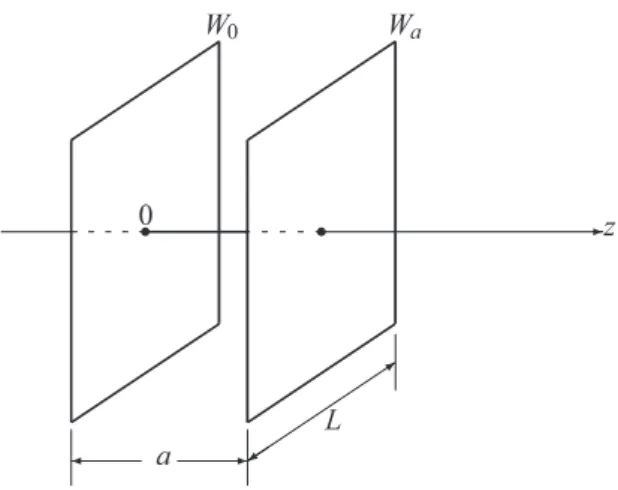
(2) 102. Fig. 1: Casimir effect between two parallel pıates W_{0} and W_{a} where \omega_{0} (resp. \omega_{I} ) is the one‐photon energy in the free space configuration (resp. in the con‐ figuration with two plates). These quantities are of course divergent and hence meaningless. Hence V is ill‐defined in its original form. Therefore one needs a regularization (renormaliza‐ tion) for V to obtain the finite result stated above (for the details of the regularization, see [10] or [22, §3‐2‐4]). In 1997, H. Ezawa et al [15] presented a different interpretation from the standard one: the Casimir force is nothming but the Lorentz force actming upon the electric current and charge in‐ duced on the plates by the quantum radiation field, suggesting an approach to the Casimir effect without invokin g zero‐point energy and in terms of representation of canonical commutation relations (CCR) inequivalent to the Fock representation. A enormous number of physics articles on Casimir effects in various configurations ofper‐ fectly conductming bodies has been published, but it seems that there have been few mathemati‐ cally rigorous studies on Casimir effects, where we mean by “a mathematically rigorous study” that it is a mathematically consistent study usin g a framework of modem mathematical quan‐ tum field theory (e.g., [5, 7, 9, 12, 16, 17, 28]) in which no use ofzero‐point energy is made. Systematic mathematically rigorous studies on the Casimir effect have been given by Herde‐ gen [ı8, 19] and Herdegen& Stopa [20]. Their approach to Casimir effects is without invoking zero‐point energies and uses concepts in algebraic quantum field theory with representations of CCR in regularized forms. A similar point of view was taken in [11]. The present work is motivated by the followin g philosophy:. The Universe uses inequivalent representations of CCR or CAR (canonical anti‐ commutation relations) to produce characteristic ”quantum‐macroscopic” phenom‐ ena.. Examples of such phenomena are: (i) Aharonov‐Bohm effect ([1] and references therein); (ii) boson masses [3]; (iii) masses of Dirac particles [4]; (iv) Bose‐Einstein condensations ([8, 14].

(3) 103 or [2, Chapter 10]); (5) superconductivity [13]. In the case ofthe Casimir effect, an interaction ofmacroscopic objects (perfectly conductming plates) with the quantum radiation field is involved. It is known that an effect similar to the Casimir effect may occur also for other quantum fields than the quantum radiation field. The word “Casimir effect” is used for such an effect too. We infer that an inequivalent representation of CCR is associated with Casimir effect. In this paper, we report that this conjecture is right in the case of a quantum scalar field. A new point in our work is that the representation of CCR we construct comes from a singular Bogoliubov transformation to which the theory ofthe standard Bogoliubov transformation (e.g., [27], [21] and references therein) cannot be applied. It is shown that the representation is inequivalent to the Fock representation of the CCR over the same inner product space. In the present paper, we describe only an outlmine of the results we have obtained. For more details, we refer the reader to paper [6]. Throughout this paper, we use the followin g notation: \bullet. For a complex inner product space. \mathscr{V} ,. we denote by {, \rangle_{\mathscr{V} (or simply {, }) the inner. product of \mathscr{V} (linear in the second variable and anti‐linear in the first) and by \Vert\cdot\Vert_{\mathscr{V} (or. \Vert\cdot\Vert) the norm of \mathscr{V}.. e. 2. For a linear operator A on a Hilbert space \mathscr{H} , we denote by D(A) the domain A^{*} the adjoint ofAifA is densely defined (i.e., D(A) is dense in \mathscr{H} ).. e. For two ımear operators. \bullet. \mathfrak{B}(\mathscr{H}). \bullet. For a linear operator. :=. A. and. B. on \mathscr{H} , their commutator is defined by [A,B]. ofA. and by. :=AB-BA.. the set of everywhere defined bounded linear operators on \mathscr{H}. A. on \mathscr{H} and a subset \mathscr{D}\subset D(A), A\mathscr{D}:=\{A\Psi|\Psi\in \mathscr{D}\}.. Representations ofthe CCR over a Complex Inner Product Space. In this section we recalı some concepts in the theory ofrepresentations of CCR. Let \mathscr{F} be a complex Hilbert space and \mathscr{D} be a dense subspace of \mathscr{F} . Let \mathscr{V} be a complex inner product space. Definition 2.1 Suppose that, for each f\in \mathscr{V} , a densely defined closed linear operator C(f) on \mathscr{F} is given. Then the triple (\mathscr{F}, \mathscr{D}, \{C(f),C(f)^{*}|f\in \mathscr{V}\}) is called a representation ofthe CCR over \mathscr{V} if the following (i)-(iii) hold: (i) (invariance) For all f\in \mathscr{V}, \mathscr{D}\subset D(C(f))\cap D(C(f)^{*}) . C(f)\mathscr{D}\subset \mathscr{D}, C(f)^{*}\mathscr{D}\subset \mathscr{F},. (ii) (anti‐linearity) For all f,g\in \mathscr{V} and \alpha,\beta\in \mathbb{C}, C(\alpha f+\beta g)=\alpha^{*}C(f)+\beta^{*}C(g) on \mathscr{D}, where, for z\in \mathbb{C}, z^{*} denotes the complex conjugate ofz. (iii) (CCR over \mathscr{V} ) For all f,g\in \mathscr{V},. [C(f),C(g)^{*}]=\langle f,g\}_{\mathscr{V}},. [C(f),C(g)]=0. on. \mathscr{D}..

(4) 104 Definition 2.2 Two representations (\mathscr{F}, \mathscr{D}, \{C(f),C(f)^{*}|f\in \mathscr{V}\}) and (\mathscr{F}', \mathscr{D}', \{C'(f), C'(f)^{*} |f\in \mathscr{V}\}) ofthe CCR over \mathscr{V} are said to be equivalent ifthere exists a unitary operator U:\mathscr{F}arrow \mathscr{F}' such that, for aıl f\in \mathscr{V},. UC(f)U^{-1}=C'(f) Remark 2.3 Operator equality (2.1) implies that \mathfrak{A}. Definition 2.4 Let. (2.1). UC(f)^{*}U^{-1}=C'(f)^{*}. be a set of(not necessarily bounded) linear operators on a Hilbert space. \mathscr{X}.. (i) The set \mathfrak{A} is said to be reducible if there is a non‐trivial closed subspace \mathscr{M} of \mathscr{X} (\mathscr{M}\neq\{0\}, \mathscr{X}) such that every A\in \mathfrak{A} is reduced by \mathscr{M} (i.e., P_{\mathscr{M} A\subset AP_{\mathscr{M},^{*} where P_{\mathscr{M} is the orthogonal projection onto \mathscr{M} ). (ii) The set. \mathfrak{A}. is said to be irreducible if it is not reducible.. Definition 2.5 A representation (\mathscr{F}, \mathscr{D}, \{C(f),C(f)^{*}|f\in \mathscr{V}\}) ofthe CCR over \mathscr{V} is said to be reducible (resp. irreducible) if the set \{C(f),C(f)^{*}|f\in \mathscr{V}\} is reducible (resp. irreducible). Definition 2.6 For a set \mathfrak{A} oflinear operators on a Hilbert space \mathscr{X},. \mathfrak{A}' :=\{T\in \mathfrak{B}(\mathscr{X})|TA\subset AT,\forall A\in \mathfrak{A}\} is called the strong commutant of \mathfrak{A}. The following fact is well known [5, Proposition 5.9]: Lemma 2.7 Let \mathfrak{A} be a set oflinear operators on \mathscr{X}.. (i) If\mathfrak{A}'=\mathbb{C}I:=\{al|a\in \mathbb{C}\} (I denotes identity), then. \mathfrak{A}. is irreducible.. (ii) If \mathfrak{A} is an irreducible set of densely defined linear operators on \mathscr{X}and* ‐invariant. (i.e., A\in \mathfrak{A}\Rightarrow A^{*}\in \mathfrak{A}) , then \mathfrak{A}'=\mathbb{C}I.. 3. Representations of CCR in Boson Fock Space. 3.1. Boson Fock space. Let \mathscr{H} be a complex Hilbert space and \otimes_{s}^{n}\mathscr{H} be the n ‐fold symmetric tensor product Hilbert space of \mathscr{H} with convention \otimes_{s}^{0}\mathscr{H}:=\mathbb{C} . Then the boson Fock space over \mathscr{H} is defined as the infinite direct sum Hilbert space of \otimes_{s}^{n}\mathscr{H}, n\geq 0 :. \mathscr{F}_{b}(\mathscr{H}):=\oplus_{n=0}^{\infty}\otimes_{s}^{n}\mathscr{H}. = \{\Psi=\{\Psi^{(n)}\}_{n=0}^{\infty}|\Psi^{(n)}\in\otimes_{s}^{n}\mathscr{H}, n\geq 0,\sum_{n=0}^{\infty}\Vert\Psi^{(n)}\Vert^{2}<\infty\}. *. For linear operators. A\Psi=B\Psi,\forall\Psi\in D(A). .. A. and. B. on. \mathscr{X} ,. “‘. A\subset B. ‘’ means that. B. is an extension of A , i.e., D(A)\subset D(B) and.

(5) 105 The subspace. \mathscr{F}_{0}(\mathscr{H}). :=. { \Psi\in \mathscr{F}_{b}(\mathscr{H})|\exists n_{0}\in \mathbb{N} such that, for all n\geq n_{0}, \Psi^{(n)}=0 }. is dense in \mathscr{F}_{b}(\mathscr{H}) and is called the finite particle subspace of \mathscr{F}_{b}(\mathscr{H}) . For each f\in \mathscr{H} , there exists a unique densely defined closed linear operator A(f) , called the annihilation operator with test vector f\in \mathscr{H} on \mathscr{F}_{b}(\mathscr{H}) , such that its adjoint A(f)^{*} , called the creation operator with test vector f\in \mathscr{H} on \mathscr{F}_{t}(\mathscr{H}) , is given as follows:. D(A(f)^{*})= \{\Psi\in \mathscr{F}_{b}(\mathscr{H})|\sum_{n=1}^{\infty}n\Vert S_{n}(f\otimes\Psi^{(n-1)} \Vert^{2}<\infty\}, (A(f)^{*}\Psi)^{(0)}=0, (A(f)^{*}\Psi)^{(n)}=\sqrt{n}S_{n}(f\otimes\Psi^{(n-1)}) , n\geq 1, \Psi\in D(A (f)^{*}). .. Basic properties ofA(f) and A(f)^{*} are summarized in the next proposition: Proposition 3.1. (i) For all f\in \mathscr{H}, \mathscr{F}_{0}(\mathscr{H})\subset D(A(f))\cap D(A(f)^{*}) and A(f) and A(f)^{*} leave \mathscr{F}_{0}(\mathscr{H}) invariant.. (ii) \{A(f),A(f)^{*}|f\in \mathscr{H}\} satisfies the CCR over \mathscr{H} :. [A(f),A(g)^{*}]=\langle f,g\}_{\mathscr{H}}, [A(f),A(g)]=0, [A(f)^{*},A(g)^{*}] =0 (f,g\in \mathscr{H}) on. \mathscr{F}_{0}(\mathscr{H}) .. The vector. \Omega_{\mathscr{H}}:=\{1,0,0, \ldots\}\in \mathscr{F}_{b}(\mathscr{H}) is called the Fock vacuum in \mathscr{F}_{b}(\mathscr{H}) . It is easy to see that. A(f)\Omega_{\mathscr{H}}=0, f\in \mathscr{H}. Let. T. be a non‐negative self‐adjoint operator on. \mathscr{H} .. Then. jth\smile. T^{(n)}:= \sum_{j=1}^{n}I\otimes\cdots\otimes I\otimes T\otimes I\cdots\otimes I is a non‐negative self‐adjoint operator on \otimes_{s}^{n}\mathscr{H} . We set T^{(0)} quantization operator of T is defined by. :=0. acting on. \mathb {C} .. The second. d\Gamma(T):=\oplus_{n=0}^{\infty}T^{(n)} actming in \mathscr{F}_{b}(\mathscr{H}) . The following theorem is well known: Theorem 3.2 The operator d\Gamma(T) is a non‐negative self‐adjoint operator and, for all t\in \mathbb{R},. e^{itd\Gamma(T)}A(f)e^{-itd\Gamma(T)}=A(e^{itT}f) , f\in \mathscr{H}. Remark3.3 The notion of second quantization operator can be extended to the case where is a densely defined closable operator on \mathscr{H}.. For more details ofthe theory ofboson Fock space, see [5, Chapter 5].. T.

(6) 106 3.2. Fock representation of CCR and related facts. Let \mathscr{V} be a dense subspace of \mathscr{H} . Proposition 3.1 implies the following fact: Proposition 3.4 The triple. \pi_{\Gamma}(\mathscr{V}):=(\mathscr{F}_{b}(\mathscr{H}),\mathscr{F}_{0} (\mathscr{H}), \{A(f),A(f)^{*}|f\in \mathscr{V}\}) is an irreducible representation of the CCR over. \mathscr{V}.. Proof. For a proof ofthe irreducibility, see [5, Theorem 5.14].. I. The representation \pi_{\Gamma}(\mathscr{V}) is called the Fock representation of the CCR over \mathscr{V}. Definition 3.5 We say that a densely defined closable linear operator Hilbert‐Schmidt if it is closable and the cıosure \overline{A} is Hilbert‐Schmidt.. A. on a Hilbert space is. The next proposition plays a basic role in the theory of representations of CCR in boson Fock spaces: Proposition 3.6 Assume that \mathscr{H} is separable. Let S and T be (not necessarily bounded) linear operators on \mathscr{H} such that there exists a dense subspace \mathscr{V} satisfying (i) \mathscr{V}\subset D(S)\cap D(T). (ii) T_{\mathscr{V} :=T\lceil \mathscr{V} (the restriction of Let. C. be a conjugation on \mathscr{H} (i. e.,. C. T. to \mathscr{V)} is injective and Ran T_{\mathscr{V} is dense in. \mathscr{H}.. is an anti‐linear mapping on \mathscr{H} such that C^{2}=I and. \Vert Cf\Vert=\Vert f\Vert, f\in \mathscr{H}) and suppose that there exists a non‐zero vector \Omega\in \mathscr{F}_{b}(\mathscr{H}) such that, for all \Psi\in \mathscr{F}_{0}(\mathscr{H}) and f\in \mathscr{V},. \{A(Tf)^{*}\Psi,\Omega\rangle=-\langle A(CSf)\Psi,\Omega\rangle. Then. ST_{\mathscr{V} ^{-1}. is Hilbert‐Schmidt.. Proof. See [3].. I. Remark3.7 In the case where T and S are in \mathfrak{B}(\mathscr{H}) , this proposition is essentially known in the context of the theory of standard Bogoliubov transformations (see, e.g., [27], [21] and references therein). Lemma 3.8 LetX and Y be (not necessarily bounded) linear operators on \mathscr{H} such that there exists a dense subspace \mathscr{V}\subset D(X)\cap D(Y) and thefollowing equation holds:. \langle Xf,Xg\rangle-\langle Yf,Yg\rangle=\langle f,g\rangle, f,g\in \mathscr{V} . LetX_{\mathscr{V}} :=Xr\mathscr{V}. Then X_{\mathscr{V} is injective. andX_{\mathscr{V} ^{-1}. is bounded with. \Vert X_{\mathscr{V} ^{-1}\Vert\leq 1.. (3.1).

(7) 107 Proof. It follows from (3.1) that, for all f\in \mathscr{V},. \Vert X_{\mathscr{V} f\Vert^{2}=\Vert f\Vert^{2}+\Vert Yf\Vert^{2}\geq\Vert f\Vert^{2}, which implies the desired result.. I. The followin g proposition plays a crucial role in the present work. Proposition 3.9 Assume that \mathscr{H} is separable. Let. X. and. Y. be as in Lemma 3.8 and suppose. that X is unbounded andX\mathscr{V} is dense in \mathscr{H} . Then there is no non‐zero vector. \Omega\in \mathscr{F}_{b}(\mathscr{H}). such that. \{A(Xf)^{*}\Psi,\Omega\rangle=-\{A(CYf)\Psi,\Omega\rangle, \Psi\in \mathscr{F}_ {0}(\mathscr{H}), f\in \mathscr{V}. Proof. This proposition can be proved by reductio ad absurdum with applications of Propo‐ sition 3.6, Lemma 3.8 and arguments on spectral properties. For the details, see [6, Proposition 3.4]. 1. 3.3. A representation of CCR defined by a singular Bogoliubov transfor‐ mation. Let T and S be densely defined (not necessarily bounded) linear operators on \mathscr{H} such that there exists a dense subspace \mathscr{V}\subset D(T)\cap D(S) and the followin g equations hold:. \{Tf, Tg\rangle-\langle Sf, Sg\}=\{f,g\rangle , \langle Tf , CSg\}=\{Sf, CTg\rangle, f,g\in \mathscr{V} ,. (3.2) (3.3). where C is a conjugation on \mathscr{H} . Then it is easy to see that, for each f\in \mathscr{V}, A(Tf)+A(CSf)^{*} is closable. Hence one can define a densely defined closed operator B(f) on \mathscr{F}_{b}(\mathscr{H}) by. B(f) :=A(Tf)+A(CSf)^{*}. Equations (3.2) and (3.3) imply that B(\cdot) and B(\cdot)^{*} satisfy the CCR over. \mathscr{V} :. for all f,g\in \mathscr{V},. [B(f),B(g)^{*}]=\langle f,g\rangle, [B(f),B(g)]=0, [B(f)^{*},B(g)^{*}]=0 on\mathscr{F}_{0}(\mathscr{H}). .. Therefore we have the foılowing fact: Proposition 3.10. \pi_{B}(\mathscr{V}):=(\mathscr{F}_{b}(\mathscr{H}), \mathscr{F}_{0} (\mathscr{H}), \{B(f),B(f)^{*}|f\in \mathscr{V}\} is a representation of the CCR over. \mathscr{V}.. Remark 3.11. (i) The correspondence T_{B}:(A(\cdot),A(\cdot)^{*})\mapsto(B(\cdot),B(\cdot)^{*}) is a generalization ofthe standard Bogoliubov transformation in the sense that S or T may be unbounded and T_{B} is not necessarily invertible..

(8) 108 (ii) Equation (3.2) impıies that. T. is bounded if and only if. S. is bounded.. Based on Remark 3.11, we say that the Bogoliubov transformation under consideration is i ngular if T or S is unbounded (then both T and S are unbounded). We emphasize that, for a s i ngular Bogoliubov transformation, the theory of the standard Bogoliubov transformation (e.g., [27], [21] and references therein) cannot be applied. s. Theorem 3.12 Assume that \mathscr{H} is separable. Suppose that T is bounded and S is not Hilbert‐ Schmidt. Then \pi_{B}(\mathscr{V}) is inequivalent to any direct sum representations of the Fock representa‐ tion \pi_{\Gamma}(\mathscr{V}) . In particular, if \pi_{B}(\mathscr{V}) is irreducible, then \pi_{B}(\mathscr{V}) is inequivalent to \pi_{F}(\mathscr{V}) .. Remark3.13 Theorem 3.12 is only a slight generalization of a well known fact in the theory of the standard Bogoliubov transformations in that \mathscr{V} is not equal to \mathscr{H} and inequivalence is about direct sum representations of the Fock representation \pi_{\Gamma}(\mathscr{V}) . Theorem 3.14 Assume that \mathscr{H} is separable. Suppose that T is unbounded and T\mathscr{V} is dense in \mathscr{H} . Then \pi_{B}(\mathscr{V}) is inequivalent to any direct sum representation of the Fock representation \pi_{F}(\mathscr{V}) . In particular, if \pi_{B}(\mathscr{V}) is irreducible, then \pi_{B}(\mathscr{V}) is inequivalent to \pi_{\Gamma}(\mathscr{V}) .. Proof. This can be proved by reductio ad absurdum. The essence of the proof is to show that, if \pi_{B}(\mathscr{V}) is equivalent to a direct sum representation of the Fock representation \pi_{\Gamma}(\mathscr{V}) , then one arrives at a contradiction with Proposition 3.9. 1. 4. A Free Quantum Scalar Field on a Finite Box. In this section, we construct a free relativistic quantum scalar field on the d‐dimensional finite box. \Lambda:=(0,L)^{d-1}\cross(0,L_{d}) =\{x=(x_{1}, \ldots,x_{d})|x_{1}, x_{d-1}\in(0,L), x_{d}\in(0,L_{d})\}, with d\geq 2, L>0 and L_{d}>0 . We consider the case where the free quantum scalar field obeys the D chlet boundary condition on the boundary of \Lambda . Hence the Hamiltonian (one‐particle Hamiıtoman) for a scalar boson is given by. h:=(-A_{D}+m^{2})^{1/2} ,. (4.1). where \Delta_{D} denotes the Dirichlet Laplacian (e.g., [25, p.263]) actming in L^{2}(\Lambda) and m\geq 0 is the mass of one boson. Then the Hamiltomian ofthe free quantum scalar field to be constructed is defined by. H:=d\Gamma(h) acting in the boson Fock space. \mathscr{F}_{b}(L^{2}(\Lambda)) over L^{2}(\Lambda) .. Remark 4.1 It is well known that -\Delta_{D} is strictly positive. Hence h is strictly positive even in the case m=0 . Therefore h is bijective with h-{\imath}\in \mathfrak{B}(L^{2}(\Lambda)) . It follows from functional calculus that. h^{-1/2}\in \mathfrak{B}(L^{2}(\Lambda)) ..

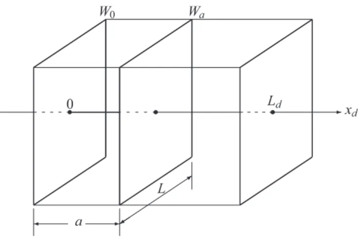
(9) 109 We denote by a(f) the annihilation operator with test vector f\in L^{2}(\Lambda) on \mathscr{F}_{b}(L^{2}(\Lambda)) and by L_{rea1}^{2}(\Lambda) the real Hilbert space consistming ofreal elements in L^{2}(\Lambda) . We take as the time‐zero fields the following operators:. \phi(f):=\frac{1}{\sqrt{2} (a(h^{-1/2}f)^{*}+a(h^{-1/2}f) , f\in L_{rea1}^{2}( \Lambda) \pi(g) :=\frac{i}{\sqrt{2} (a(h^{1/2}g)^{*}-a(h^{1/2}g) , g\in D(h^{{\imath} /2})\cap L_{rea1}(\Lambda) ,. .. Then the time t‐fields with the Hamiltonian H are defined as follows:. \phi(t,f):=e^{itH}\phi(f)e^{-itH}, f\in L_{rea1}^{2}(\Lambda) \pi(t,g) :=e^{itH}\pi(g)e^{-itH}, g\in D(h^{1/2})\cap L_{rea1}(\Lambda) , t\in \mathbb{R}. ,. By Theorem 3.2, we obtain the following proposition: Proposition 4.2 For all t\in \mathbb{R},. \phi(t,f)=\phi(e^{ith}f) , \pi(t,g)=\pi(e^{ith}g) , f\in L_{rea1}^{2}(\Lambda), D(h^{1/2})\cap L_{rea1}^{2}(\Lambda). .. One can show that (\phi(t,f), \pi(t,g)) obeys the following functional field equations:. \frac{d}{dt}\phi(t,f)\Psi=\pi(t,f)\Psi,. \frac{d^{2} {dt^{2} \phi(t,f)\Psi-\phi(t,\Delta_{D}f)\Psi+m^{2}\phi(t,f)\Psi=0 for all. \Psi\in \mathscr{F}_{0}(L^{2}(\Lambda)) and f\in D(h^{2})\cap L_{rea1}^{2}(\Lambda) , where the time derivatives d/dt and d^{2}/dt^{2} are. taken in the strong sense. Thus \phi(t, \cdot) is a free quantum scalar field obeying the Klein‐Gordon equation on \Lambda with D chlet boundary condition.. 5. A Quantum Scalar Field on A with a Partition by a Per‐ fectly‐Conducting Wall. We next consider the case where a perfectly conducting wall (plate). W_{a}:=\{x\in\Lambda|x_{d}=a\} perpendicular to the. x_{d} ‐axis. is placed in \Lambda with 0<a<L_{d} (see Fig.2). The box \Lambda is decomposed. as. \Lambda=\Lambda_{1}\cup W_{a}\cup\Lambda_{2}, where. \Lambda_{1} :=\{x\in\Lambda|0<x_{d}<a\}, \Lambda_{2} :=\{x\in\Lambda|a<x_{d}<L_ {d}\}. Correspondming to this decomposition,. L^{2}(\Lambda) has the orthogonal decomposition. L^{2}(\Lambda)=L^{2}(\Lambda_{1})\oplus L^{2}(\Lambda_{2}) We denote by \Delta_{\el } the Dirichlet Laplacian for \Lambda p, \ell=1,2.. ..

(10) 110. Fig. 2: Box. \Lambda. with partition W_{a}. Remark 5.1 The D chlet Laplacian \Delta_{D} can not be reduced by L^{2}(\Lambda_{\ell})(\ell=1,2) . This suggests that the presence of W_{a} may give rise to physics different from that of the system without W_{a} even if no other interactions exist. This may be a mathematical origin of the Casimir effect in the present context. We take as one‐particle Hamiltonian with the wall W_{a} the following operator:. h_{a}:=h_{a,1}\oplus h_{a,2}, where. h_{a,\ell}:=(-\Delta_{\ell}+m^{2})^{1/2} on. L^{2}(\Lambda_{\ell}) . In what follows, we assume the following:. Assumption (a) The number. 5.1. L^{2}/L_{d}^{2}\in \mathbb{Q} is a rational number, but a^{2}/L_{d}^{2} is an irrational one.. Some properties of the Dirichlet one‐particle Hamiltonians and re‐ lated facts. Let. \Gam a:=(\frac{\pi}{L}\mathb {N})^{d-1}\cros \frac{\pi}{L_{d} \mathb {N}. = \{k=(k_{1}, \ldots,k_{d})|k_{j}\in\frac{\pi}{L}\mathbb{N},j=1, d-1, k_{d} \in\frac{\pi}{L_{d} \mathbb{N}\}.

(11) 111 111 For each k\in\Gamma and \ell=1,2 , we define functions. \psi_{k}^{(\el )} on \Lambda_{\el} as follows:. \psi_{k}^{(1)}(x):=(\prod_{j=1}^{d-1}\varphi_{k_{j} (x_{j}) \psi_{k_{d} ^{(1)} (x_{d}) , x\in\Lambda_{1}, \psi_{k}^{(2)}(x):=(\prod_{j=1}^{d-1}\varphi_{k_{j} (x_{j}) \psi_{k_{d} ^{(2)} (x_{d}) , x\in\Lambda_{2}, where. \varphi_{k_{j} (x_{j}):=\sqrt{\frac{2}{L} \sin(k_{j}x_{j}) , x_{j}\in(0,L), j= 1, d-1, \psi_{k_{d} ^{(1)}(x_{d}):=\sqrt{\frac{2}{a} \sin\frac{L_{d}k_{d}x_{d} {a}, x_ {d}\in(0,a) \psi_{k_{d} ^{(2)}(x_{d}):=\sqrt{\frac{2}{L-a} \sin\frac{L_{d}k_{d}(x_{d}-a)} {L_{d}-a}, x_{d}\in(a,L_{d}) ,. .. Then. (-\Delta_{\ell}+m^{2})\psi_{k}^{(\ell)}=\omega_{\ell}(k)^{2}\psi_{k}^{(\ell)}, k\in\Gamma, where. \omega_{1}(k):=\sqrt{k_{1}^{2}++k_{d-1}^{2}+(L_{d}k_{d}/a)^{2}+m^{2} , \omega_{2}(k):=\sqrt{k_{1}^{2}++k_{d-1}^{2}+(L_{d}k_{d}/(L_{d}-a))^{2}+m^{2}}. The set. \{\psi_{k}^{(\el )}\}_{k\in\Gamma} is a CONS ofL^{2}(\Lambda_{\ell}) . One has. h_{a,\ell}\psi_{k}^{(\ell)}=\omega_{\ell}(k)\psi_{k}^{(\ell)} Each. or. f\in L^{2}(\Lambda). f=(f^{(1)},f^{(2)}). is written as. f=f^{(1)}+f^{(2)}. with. f^{(\ell)}:=\chi_{\Lambda_{\ell} f\in L^{2}(\Lambda_{\ell}). ,. where \chi_{\Lambda_{\el } is the characteristic function of \Lambda_{\el } . The direct sum operator of -\Delta_{1} and -\Delta_{2}. -\Delta_{12}:=(-A_{1})\oplus(-\Delta_{2}) is a strictly positive self‐adjoint operator on. L^{2}(\Lambda) . By functional calculus, we have. (-\Delta_{12})^{1/2}=(-\Delta_{1})^{1/2}\oplus(-\Delta_{2})^{1/2}. Lemma 5.2. D((-\Delta_{12})^{1/2})\subset D((-\Delta_{D})^{1/2}). and, for all. f\in D((-\Delta_{12})^{1/2}) ,. \Vert(-\Delta_{D}) ı/2 f\Vert=\Vert(-\Delta_{12})^{1/2}f\Vert . In particular,. (-\Delta_{D})^{1/2}(-\Delta_{{\imath} 2})^{-1/2}. is an everywhere defined bounded operator on. (5.1) L^{2}(\Lambda) ..

(12) 112 Lemma 5.3. (i) D(h_{a})\subset D(h) and (ii). hh_{a}^{-1}\in \mathfrak{B}(L^{2}(\Lambda)) .. D(h_{a}^{1/2})\subset D(h^{1/2}) and h^{1/2}h_{a}^{-1/2}\in \mathfrak{B}(L^{2}(\Lambda)) .. For convemience, we extend the function. \psi_{k}^{(\el )} to a function on \Lambda :. \tilde{\psi}_{k}^{(\el)}(x):=\{ begin{ar y}{l \psi_{k}^{(\el)}(x) ifx\in\Lambda_{\el} 0 ifx\in\Lambda\backsla h\Lambda_{\el} \end{ar y} For aıı. \alpha\in \mathbb{R},. h_{a}^{\alpha}\tilde{\psi}_{k}^{(\ell)}=\omega_{\ell}(k)^{\alpha}\tilde{\psi} _{k}^{(\ell)}, \ell=1,2, k\in\Gamma. For each (k,p)\in\Gamma\cross\Gamma , one has. \langle\varphi_{k},\tilde{\psi}_{p}^{(\el)}\rangle=(\prod_{j=1}^{d-1} \delta_{k_{j}p_{j})\langle\varphi_{k_{d},\tilde{\psi}_{p_{d}^{(\el)}\rangle. .. (5.2). We set. cı. Lemma 5.4 For all. := \frac{L_{d} {a}, c_{2}:= \frac{L_{d} {L_{d}-a}.. k_{d}, p_{d}\in(\pi/L_{d})\mathbb{N},. \langle\varphi_{k_{d},\tilde{\psi}_{p_{d}^{(\imath})\rangle=\frac{2}{\sqrt {L_{d}a \frac{(-1)^{L_{d}p_{d}c_{\imath}p_{d}s\dot{m}(ak_{d}){k_{d}^{2}- c_{1}^{2}p_{d}^{2}, \langle\varphi_{k_{d} ,\tilde{\psi}_{p_{d} ^{(2)}\rangle=-\frac{2}{\sqrt{L_{d} (L_{d}-a)} \frac{ _{2}p_{d}s\dot{m}(ak_{d}) {k_{d}^{2}-c_{2}^{2}p_{d}^{2} . Lemma 5.5. D(h_{a}^{1/2})_{\neq}^{\subset}D(h^{1/2}) .. Proof. One can show that, for some k_{0}\in\Gamma, and Lemma 5.4 to estimate some quantity).. \varphi_{k_{0} \not\in D(h_{a}^{1/2}) (this is non‐trivial; we use (5.2) I. The followin g fact shows a singuıar nature of the pair (h,h_{a}) of one‐particle Hamiltonians: Lemma 5.6 The operator. h^{-1/2}h_{a}^{1/2}. is unbounded.. Proof. Let T :=h^{-1/2}h_{a}^{1/2} We prove the unboundedness of T by reductio ad absurdum. Suppose that T were bounded. Since D(T)=D(h_{a}^{1/2}), T is densely defined. Hence it is closable and the closure \overline{T} is everywhere defined bounded operator on L^{2}(\Lambda) . We have T^{*}=(\overline{T})^{*}. Hence D(T^{*})=L^{2}(\Lambda) . Since h^{-1/2} is bounded with D(h^{-{\imath}/2})=L^{2}(\Lambda) , it follows that T^{*}=. (h_{a}^{1/2})^{*}(h^{-1/2})^{*}=h_{a}^{1/2}h^{-1/2} . This implies that D(h^{1/2})\subset D(h_{a}^{1/2}) and D(T^{*})=h^{1/2}D(h_{a}^{1/2}) . 1 D(h^{1/2})=D(h_{a}^{1/2}) . But this contradicts Lemma 5.5.. Hence, by Lemma 5.3(ii),.

(13) 113 Lemma 5.7 Let. s_{\pm:=\frac{1}{2}(h^{-1/2}h_{a}^{1/2}\pm h^{1/2}h_{a}^{-1/2})}. Then s_{\pm}are unbounded.. Proof. This follows from Lemma 5.3(ii) and Lemma 5.6. We note that. \mathscr{V}_{a} :=D(S_{+})=D(S_{-})=D(h_{a}^{1/2}). 1 .. Lemma 5.8 For all f,g\in \mathscr{V}_{a} , thefollowing equations hold.‘. \langle S_{+}f,S_{+}g\}-\langle S_{-}f,S_{-}g\rangle=\{f,g\rangle, \langle S_{+}f,S_{-}g\}=\{S_{-}f,S_{+}g\rangle. Proof. These equations follow from direct computations. Lemma 5.9 The range RanS_{+}ofS_{+}is dense in. 5.2. I. L^{2}(\Lambda) .. A singular Bogoliubov transformation and a representation of the CCR over a dense subspace. We denote by C_{\Lambda} the complex conjugation on. L^{2}(\Lambda) :. C_{\Lambda}f:=f, f\in L^{2}(\Lambda). .. We define. b(f):=a(S_{+}f)+a(C_{\Lambda}S_{-}f)^{*}, f\in \mathscr{V}_{a} .. (5.3). It is easy to see that, for all f,g\in \mathscr{V}_{a},. [b(f),b(g)^{*}]=\langle f,g\}, [b(f),b(g)]=0, [b(f)^{*}, b(g)^{*}]=0 on \mathscr{F}_{0}(L^{2}(\Lambda)) . The correspondence: (a(\cdot),a(\cdot)^{*})\mapsto(b(\cdot), b(\cdot)^{*}) is a Bogoliubov transforma‐ tion. But, by Lemma 5.7, this is a singular Bogoliubov transformation. The linear hull. \mathscr{E}:=1.h.\{\tilde{\psi}_{k}^{(\ell)}|k\in\Gamma, \ell=1,2\} ofthe subset \{\tilde{\psi}_{k}^{(\ell)}|k\in\Gamma, \ell=1,2\} is dense in L^{2}(\Lambda) . For all \alpha>0, \mathscr{E}\subset D(h_{a}^{\alpha}) with h_{a}^{\alpha}\tilde{\psi}_{k}^{(\ell)}=\omega_{\ell}(k)^{\alpha}\tilde{\psi} _{k}^{(\ell)}, k\in\Gamma, \ell=1,2.. (5.4). Hence. h_{a}^{\alpha}\mathscr{E}\subset \mathscr{E} .. (5.5). Lemma 5.10 The triple. \pi_{b}(\mathscr{E}):=(\mathscr{F}_{b}(L^{2}(\Lambda)), \mathscr{F}_{0}(L^{2} (\Lambda)), \{b(f), b(f)^{*}|f\in \mathscr{E}\}) is a representation of the CCR over. \mathscr{E}.. ..

(14) 114 5.3. A quantum scalar field on. \Lambda. with W_{a}. We now introduce the following operators:. \phi_{b}(f):=\frac{{\imath} {\sqrt{2} (b(h_{a}^{-1/2}f)^{*}+b(h_{a}^{-1/2}f) , f\in L_{rea1}^{2}(\Lambda) \pi_{b}(g):=\frac{i}{\sqrt{2} (b(h_{a}^{1/2}g)^{*}-b(h_{a}^{1/2}g) , g\in D(h_{a})\cap L_{rea1}^{2}(\Lambda) ,. Lemma 5.11 For all. (5.6) .. (5.7). f\in D(h^{1/2})\cap D(h_{a})\cap L_{reai}^{2}(\Lambda) , \phi_{b}(f)=\phi(f). \pi_{b}(f)=\pi(f). ,. on. \mathscr{F}_{0}(L^{2}(\Lambda)). .. For each t\in \mathbb{R} , we define. \phi_{b}(t,f):=\phi_{b}(e^{ith_{a}}f) , f\in L_{rea1}^{2}(\Lambda) ,. (5.8). \pi_{b}(t,g):=\pi_{b}(e^{ith_{a}}g) , g\in D(h_{a}^{1/2})\cap L_{rea1}^{2} (\Lambda) .. (5.9). Note that the time‐zero fields coincide:. \phi_{b}(0,f)=\phi(f) ,. \pi_{b}(0,g)=\pi(g). on. \mathscr{F}_{0}(L^{2}(\Lambda)) .. One can show that the following field equations hold:. \frac{d^{2} {dt^{2} \phi_{b}(t,f)+\phi_{b}(t, (-\Delta_{12}+m^{2})f)=0 and. \frac{d}{dt}\phi_{b}(t,f)=\pi_{b}(t,f) on. \mathscr{F}_{0}(L^{2}(\Lambda)) ,. The quantum fields \phi_{b}(t, \cdot) and \pi_{b}(t, \cdot) have the followin g explicit forms:. \phi_{b}(t,f)=\frac{1}{\sqrt{2} (a(K(t)f)^{*}+a(K(t)f) , f\in L_{rea1}^{2} (\Lambda) \pi_{b}(t,g)=\frac{i}{\sqrt{2} (a(L(t)g)^{*}-a(L(t)g) , g\in D(h_{a})\cap L_{rea1}^{2}(\Lambda) ,. on \mathscr{F}_{0}(\mathscr{H}_{1}) , where. K(t) :=h^{-1/2}\cos(th_{a})+ih^{1/2}h_{a}^{-1}\sin(th_{a}) L(t) :=h^{1/2}\cos(th_{a})+ih^{-{\imath}/2}h_{a}\sin(th_{a}) , t\in \mathbb{R}. ,. One can define operator‐valued mappings \phi_{0} and \phi_{b,0} from operators on \mathscr{F}_{b}(L^{2}(\Lambda)) by. \mathbb{R}\cros L_{rea1}^{2}(\Lambda). \phi_{0}(t,f):=\phi(t,f)t\mathscr{F}_{0}(L^{2}(\Lambda)) \phi_{b,0}(t,f):=\phi_{b}(t,f)[\mathscr{F}_{0}(L^{2}(\Lambda)) , (t,f)\in \mathbb{R}\cross L_{rea1}^{2}(\Lambda). to the set of linear. ,. .. The followin g proposition shows that \phi_{b,0} describes a dynamics different from that of \phi_{0} :.

(15) 115 Proposition 5.12. \phi_{0}\neq\phi_{b,0} .. (5.10). Remark 5.13 Unfortunately we have been unable to make it clear if there is a self‐adjoint operator (a Hamiltomian) H_{a} on \mathscr{F}_{b}(L^{2}(\Lambda)) such that, for all t\in \mathbb{R},. e^{itH_{a}}\phi_{b}(0,f)e^{-itH_{a}}=\phi_{b}(t,f) , e^{itH_{a}}\pi_{b}(0,f)e^{ -itH_{a}}=\pi_{b}(t,f) for all f in a suitable dense subspace not exist.. 6. ofL_{rea1}^{2}(\Lambda) .. We conjecture that such an operator H_{a} does. Inequivalence of \pi_{b}(\mathscr{E}) to the Fock Representation of the CCR over \mathscr{E} on. \mathscr{F}_{b}c(L^{2}(\Lambda)). The Fock representation of the CCR over. \mathscr{E}. on. \mathscr{F}_{b}(L^{2}(\Lambda)) is given by. \pi_{\Gamma}(\mathscr{E}):=(\mathscr{F}_{b}(L^{2}(\Lambda)), \mathscr{F}_{0}(L^ {2}(\Lambda)), \{a(f),a(f)^{*}|f\in \mathscr{E}\}) Theorem 6.1 The representation \pi_{b}(\mathscr{E}) of the CCR over the Fock representation \pi_{\Gamma}(\mathscr{E}) .. \mathscr{E}. .. is irreducible and inequivalent to. Proof. We first prove the irreducibility of \pi_{b}(\mathscr{E}) . Let T\in\{b(f), b(f)^{*}|f\in \mathscr{E}\}' . Then, by (5.6), (5.7) and (5.5), T\in\{\phi_{b}(f), \pi_{b}(f)|f\in \mathscr{E}\cap L_{rea{\imath}}^{2}(\Lambda) \}' . Then we obtain. T\in\{\phi(f)[\mathscr{F}_{0}(L^{2}(\Lambda)), \pi(f)r\mathscr{F}_{0}(L^{2} (\Lambda))|f\in \mathscr{E}\cap L_{rea1}^{2}(\Lambda)\}', where we have used the fact that. \mathscr{E}\subset D(h_{a}^{1/2})\subset D(h^{1/2}) .. Recall that. \phi(f) and \pi(f) . Hence it follows from a limitming argument that. \mathscr{F}_{0}(L^{2}(\Lambda)). is a core for. T\in\{\phi(f), \pi(f)|f\in \mathscr{E}\cap L_{rea1}^{2}(\Lambda)\}'. But the right hand side is \mathbb{C}I (essentially due to [24, p.232. Lemma 1]; for a direct proof, see [5, p.289, Example 5.17]). Hence \{b(f), b(f)^{*}|f\in \mathscr{E}\}'=\mathbb{C}I . Thus \{b(f),b(f)^{*}|f\in \mathscr{E}\} is irreducible.. We next show that \pi_{b}(\mathscr{E}) is inequivalent to \pi_{\Gamma}(\mathscr{E}) . By Lemmas 5.7−5.9 and the irreducibil‐ ity of \pi_{b}(\mathscr{E}) proved in the precedin g paragraph, we can apply Theorem 3.14 to conclude that I \pi_{b}(\mathscr{E}) is inequivalent to \pi_{\Gamma}(\mathscr{E}) .. 7. Concluding Remark. We conjecture that the Casimir force in the present context can be described in terms of the representation \pi_{b}(\mathscr{E}) without invokin g zero‐point energies..

(16) 116 References [ı] A. Arai, Representation‐theoretic aspects oftwo‐dimensional quantum systems in singular vector potentials: canonical commutation relations, quantum algebras, and reduction to lattice quantum systems, J. Math. Phys. 39 (1998), 2476‐2498. [2] A. Arai, Mathematics of Quantum Statistical Mechanics, in Japanese. Kyoritsu‐shuppan, Tokyo, 2008.. [3] A. Arai, A family ofinequivalent Weyl representations ofcanonical commutation relations with applications to quantum field theory, Rev. Math. Phys. 28 (2016), 1650007 (26 pages). [4] A. Arai, Inequivalence ofquantum Dirac fields ofdifferent masses and the underlying gen‐ eral structures involved, Functional Analysis and Operator Theory for Quantum Physics, 31−53, EMS Ser. Congr. Rep., Eur. Math. Soc., Zurich, 2017.. [5] A. Arai, Analysis on Fock Spaces and Mathematical Theory of Quantum Fields, World Scientific, Singapore, 2018. [6] A. Arai, Inequivalent representation of canonical commutation relations in relation to Casimir effect, Hokkaido University Preprint Series in Mathematics, 1118 (2018). http://hdl.handle.net/2115/71731. [7] H. Araki, Mathematical Theory of Quantum Fields, Oxford University Press, Oxford, 1999; the original Japanese edition was published in 1993 (Iwanami‐shoten, Tokyo). [8] H. Araki and E. J. Woods, Representations of the canonical commutation relations de‐ scribing a nonrelativistic infinite free Bose gas, J. Math. Phys. 4 (1963), 637‐662. [9] N. N. Bogoliubov, A. A. Logonov and I. T. Todorov, Introduction to Axiomatic Quantum Field Theory, Benjamin, Readming Mass, 1975.. [10] H. B. G. Casimir, On the attraction between two perfectly conducting plates, Proc. Konin‐ klijke Nederlandse Akademie van Wetenschappen 51 (1948), 793‐795. [11] C. Dappiaggi, G. Nosari and N. Pinamonti, The Casimir effect from the point of view of algebraic quantum field theory, Math. Phys. Anal. Geom.19 (2016), 12 (44 pages). [12] J. Dereziński, J. and C. Gérard, Mathematics of Quantization and Quantum Fields, Cam‐ bridge University Press, Cambridge, 2013. [13] H. Ezawa, The representation of canonical variables as the limit of infinite space volume: the case ofthe BCS model, J. Math. Phys. 5 (1964), 1078‐1090. [14] H. Ezawa, Quantum mechanics of a many‐boson system and the representation of canon‐ ical variables, J. Math. Phys. 6 (1965), 380‐404. [15] H. Ezawa, K. Nakamura and K. Watanabe, The Casimir Force from Lorentz’s, in Frontiers in Quantum Physics (S. C. Lim, R. Abd‐Shukor, K. H. Kwek eds.), Springer, Singapore, 1998, 160‐169..

(17) 117 [16] J. Glimm and A. Jaffe, Quantum Physics, Second Edition, Springer‐Verlag, New York, 1987.. [17] R. Haag, Local Quantum Physics, Springer, Berım Heidelberg, 1992, ı996. [18] A. H. Herdegen, Quantum backreaction (Casimir) effect I. What are admissible idealiza‐ tions?, Ann. Henri Poincaré 6 (2005), 657‐695. [19] A. H. Herdegen, Quantum backreaction (Casimir) effect II. Scalar and electromagnetic fields, Ann. Henri Poincaré 7 (2006), 253‐301. [20] A. H. Herdegen and M. Stopa, Global versus local Casimir effect, Ann. Henri Poincaré 11 (2010), 1171‐1200. [21] F. Hiroshima, I. Sasaki, H. Spohn and A. Suzuki, Enhanced Binding in Quantum Field Theory, COE Lecture Note Vol. 38, Institute ofMathematics for Industry, Kyushu Univer‐ sity, 2012. [22] C. Itzykson and J.‐B. Zuber, Quantum Field Theory, McGraw‐Hill, New York, 1980. [23] S. K. Lamoreaux, Demonstration ofthe Casimir force in the 0.6 to 6 \mu m range, Phys. Rev. Lett. 78 (1998), 5−8; Erratum Phys. Rev. Lett. 81 (1998), 5475‐5476. [24] M. Reed and B. Simon, Methods of Modern Mathematical Physics II: Fourier Analysis, Self‐Adjointness, Academic Press, New York, 1975. [25] M. Reed and B. Simon, Methods ofModern Mathematical Physics IV. Analysis ofOpera‐ tors, Academic Press, New York, 1978.. [26] M. J. Sparnaay, Measurements of attractive forces between flat plates, Physica 24 (1958), 751−764.. [27] D. Shale, Linear symmetries of free boson fields, Trans. Amer. Math. Soc., 103 (1962), 149‐167.. [28] R. F. Streater and A. S. Wightman, PCT Spin and Statistics, and All That, Benjamin, Readming Mass, 1964..

(18)